Adjusting for Heritable Covariates Can Bias Effect Estimates in Genome-Wide Association Studies

Abstract

In recent years, a number of large-scale genome-wide association studies have been published for human traits adjusted for other correlated traits with a genetic basis. In most studies, the motivation for such an adjustment is to discover genetic variants associated with the primary outcome independently of the correlated trait. In this report, we contend that this objective is fulfilled when the tested variants have no effect on the covariate or when the correlation between the covariate and the outcome is fully explained by a direct effect of the covariate on the outcome. For all other scenarios, an unintended bias is introduced with respect to the primary outcome as a result of the adjustment, and this bias might lead to false positives. Here, we illustrate this point by providing examples from published genome-wide association studies, including large meta-analysis of waist-to-hip ratio and waist circumference adjusted for body mass index (BMI), where genetic effects might be biased as a result of adjustment for body mass index. Using both theory and simulations, we explore this phenomenon in detail and discuss the ramifications for future genome-wide association studies of correlated traits and diseases.

Main Text

Adjustment for covariates or correlated secondary traits in genome-wide association studies (GWASs) can have two purposes: first, to account for potential confounding factors that can bias SNP effect estimates, and second, to improve statistical power by reducing residual variance. For example, researchers routinely adjust for principal components of individual genotypes to account for population structure,¹ or principal components of gene expression to capture batch effects in gene-expression analysis.² Besides confounding factors, human traits can also be adjusted for correlated environmental or demographic factors such as gender and age to increase statistical power.^3,4 The intuition here is that accounting for a true risk factor decreases the residual variance of the outcome and therefore increases the ratio of the true effect size of a predictor of interest over the total phenotypic variance, which leads to increased statistical power.

Recently, researchers have conducted GWAS of human traits and diseases while adjusting for other heritable covariates with the motivation of identifying genetic variants associated only with the primary outcome.^5–9 An important difference between environmental/demographic factors and heritable human traits is that the latter have genetic associations. Therefore, a genetic variant can in theory be associated with both the primary outcome and the covariate used for adjustment. When that happens, the adjusted and unadjusted estimated effects of the genetic variant on the outcome will differ. If the correlation between the covariate and the outcome results from a direct effect of the covariate on the outcome (Figure 1A), the adjusted and unadjusted estimates correspond to the direct (i.e., not mediated through the covariate) and total (i.e., direct + indirect) genetic effect of the variant on the outcome, respectively. In all other situations where the observed correlation is due to shared genetic and/or environmental risk factors, the adjusted estimate can be biased relative to the true direct effect.

Figure 1.

Underlying Causal Diagrams

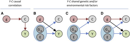
Four causal diagrams describing the causal relationship between the genotypes G, environment E, a covariate C, and the outcome of interest Y are shown. In (A), the correlation between Y and C is due to a direct effect of C on Y, whereas in (B)–(D,) the correlation between Y and C is explained by shared risk factors.

To understand when a bias is introduced, consider the causal diagrams for a single genetic variant g, an outcome of interest Y, and a covariate C (Figures 1B–1D). Besides the genetic variant in question, the two variables, Y and C, are influenced by either other genetic loci, which we denote by G_-g, or other environment factors and noise, denoted by E. For simplicity, assume that the genetic variant g and other causal factors, G_-g and E, are uncorrelated. Furthermore, assume that the covariate C and the outcome of interest, Y are correlated through (G_-g,E). If we are interested in estimating the direct effect of g on Y (the black arrow in Figure 1), then in scenario from Figure 1B adjusting for the covariate C does not bias the effect estimate and increases the power as we implicitly adjust for some environmental and other (uncorrelated) shared genetic effects. However, in scenario from Figure 1C where g only influences the covariate and not the outcome, adjusting for the covariate induces an association between the genetic variant and Y. The strength of this association depends on ρ_CY, the correlation between the covariate and the outcome due to shared risk factors, and the strength of β_C, the effect of the genetic variant on the covariate. For normalized g, C, and Y with mean 0 and variance 1, the bias of the genetic effect estimate, ${\hat{\beta }}_Y$, on the covariate adjusted trait is approximately equal to −β_Cρ_CY when β_C is small and sample size is sufficiently large (see Appendix A). Finally, consider scenario from Figure 1D, where both the covariate and the outcome are influenced by the genetic variant. Here, the association between the genetic variant and the covariate will bias the estimated genetic effect on the outcome by the same amount as before, i.e., −β_Cρ_CY. This bias observed is illustrated in Figure 2A, and as expected, it is well approximated by the product between the direct genetic effect estimate on the covariate and the correlation between the outcome and the covariate. As shown in Figure 2B, this bias leads to increased false discovery rates under the null (no direct effect of the genetic variant on the outcome). This phenomenon also implies that when there truly is a direct genetic effect on the outcome, the adjusted statistical test can have increased power to detect the genetic variant, as compared to the unadjusted test, if the genetic effect and the phenotypic correlation are in opposite directions (Figure S2, left panel). Conversely, if the genetic effect and the correlation are in the same direction, the adjusted statistical test has, in many cases, a decreased power to detect the genetic variant (Figure S2, right panel).

Figure 2.

Effect Estimates and False Discovery Rate

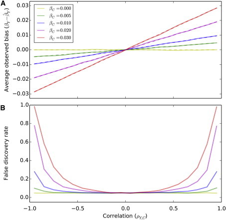
Results for simulations of correlated outcomes and covariates and a genetic variant that influences the covariate only are shown. In (A), the average observed bias of the genetic effect estimate in the covariate adjusted analysis is plotted as a function of the correlation between the outcome and the covariate for different values of direct genetic effect on the covariate. The dashed lines correspond to the theoretical bias as derived in the method section. In (B), the average false discovery rate (α = 0.05) of over 5,000 replicates is plotted as a function of ρ_Y,C the correlation between the outcome and the covariate for different values of direct genetic effect on the covariate when simulating 2,000 individuals.

The difficulty of estimating direct effects of genetic variants on a covariate-adjusted outcome is well appreciated in causal inference literature¹⁰ and by many epidemiologists,^11–13 but has received little attention in the context of GWASs.¹⁴ In Appendix B, we review 15 scenarios depicted as direct acyclic graphs in Figure S1 where adjusting for a covariate is either recommended or not and validated the interpretation of each case through simulation (see Table S3). In the absence of a clear underlying causal model or diagram, one cannot guarantee that effect estimates for covariate adjusted outcomes correspond to the desired estimates (e.g., direct versus total genetic effect). In GWASs, the potential presence of bias due to adjustment is proportional to the product of β_C and ρ_CY. Hence, adjusting for a covariate that does not have a genetic component, such as an environmental exposure, will not bias the estimate for the genotype effect on the outcome of interest as β_C = 0. On the other hand, when adjusting for a covariate that has a genetic component (potentially β_C ≠ 0), then the adjusted association signals can be difficult to interpret, because it does not necessarily imply an association with the outcome of interest only but can correspond also to a bivariate signal on Y and C, or in some extreme case to an association with the covariate only. Therefore, unless we can unequivocally determine which model in Figure 1 is the right one or rule out an effect from the genetic variant on the covariate, the reported adjusted associations should be considered with caution.

For illustrative purpose, we considered the SNPs reported to be associated at genome-wide significance levels with waist hip ratio (WHR) or waist circumference (WC), after adjustment on BMI.^6,8 The observed correlations between BMI and WHR and between BMI and WC in the GIANT data are 0.49 and 0.85, respectively (see Appendix C). Table 1 displays the gender-specific significant SNPs from these studies and the summary statistics that we extracted from the GIANT consortium website. It shows that SNPs harboring opposite marginal effects on the two traits are significantly enriched (p = 0.005). This agrees well with theory and our simulations showing increased power when the SNP has effect in opposite directions on the outcome and the covariate (Figure S2A). In the absence of a genetic effect on BMI, we expect the number of SNPs with opposite directions of effect estimates to follow a binomial distribution with probability of 0.5 (see Appendix C and Figure S3). The observed enrichment of SNPs with opposite directions indicates that a substantial fraction of those SNPs are associated with BMI in the opposite direction. Indeed, when removing the SNPs with the most significant marginal associations with BMI, the fraction of variants displaying an opposite effect becomes non-significant (Figure S4). None of the SNPs with opposite effects on BMI and either WHR or WC show significant marginal association with BMI after correction for multiple testing (although 5 out of 23 are nominally significant). However, as shown in Figure S2B, even non-significant genetic effects on the covariate can influence power when correlation between the outcome and the covariate is large (e.g., ≥ 0.5).

Table 1.

Estimates and p Values of Genetic Effects from the GIANT Study for Genetic Variants Found Associated with Waist to Hip Ratio and Waist Circumference after Adjusting for Body Mass Index

MarkerName	A1	A2	Frequency	Estimated Effects						Opposite Effect	Reference	Pβ.deviationa
WHR adjusted for BMI in women				BMI (pval)		WHR (pval)		WHRadjBMI(pval)
rs9491696	c	g	0.4800	−0.0068	(2.7E-01)	−0.0479	(1.0E-11)	−0.0472	(1.6E-12)		Heid et al.	0.81
rs6905288	a	g	0.5620	−0.0083	(2.4E-01)	0.0484	(4.7E-10)	0.0523	(7.7E-13)	X	Heid et al.	0.22
rs984222	c	g	0.6350	0.0108	(8.5E-02)	-0.0284	(9.0E-05)	-0.0359	(1.2E-07)	X	Heid et al.	0.012
rs1055144	t	c	0.2100	-0.0126	(1.1E-01)	0.0314	(4.2E-04)	0.0398	(2.3E-06)	X	Heid et al.	0.021
rs10195252	t	c	0.5990	-0.0184	(3.3E-03)	0.0447	(7.0E-10)	0.0529	(6.3E-15)	X	Heid et al.	0.0061
rs4846567	t	g	0.7170	0.0098	(1.4E-01)	-0.0543	(5.3E-12)	-0.0641	(4.7E-18)	X	Heid et al.	0.0025
rs1011731	a	g	0.4280	−0.0058	(3.5E-01)	−0.0280	(7.0E-05)	−0.0284	(2.1E-05)		Heid et al.	0.89
rs718314	a	g	0.2590	0.0077	(2.7E-01)	−0.0444	(3.9E-08)	−0.0467	(8.3E-10)	X	Heid et al.	0.49
rs1294421	t	g	0.6130	−0.0007	(9.1E-01)	−0.0357	(1.2E-06)	−0.0380	(3.4E-08)		Heid et al.	0.45
rs1443512	a	c	0.2390	−0.0014	(8.5E-01)	0.0415	(7.6E-07)	0.0479	(1.4E-09)	X	Heid et al.	0.063
rs6795735	t	c	0.5940	0.0114	(6.4E-02)	-0.0264	(2.2E-04)	-0.0330	(7.9E-07)	X	Heid et al.	0.023
rs4823006	a	g	0.5690	0.0046	(4.6E-01)	0.0337	(3.4E-06)	0.0366	(6.9E-08)		Heid et al.	0.33
rs6717858	t	c	0.5417	-0.0185	(3.1E-03)	0.0439	(8.1E-10)	0.0536	(2.8E-15)	X	Randall et al.	0.00072
rs2820443	t	c	.	-0.0099	(1.4E-01)	0.0544	(4.8E-12)	0.0643	(3.7E-18)	X	Randall et al.	0.0025
rs1358980	t	c	0.4500	-0.0148	(3.8E-02)	0.0498	(7.1E-10)	0.0565	(1.1E-13)	X	Randall et al.	0.041
rs2371767	c	g	0.2083	0.0199	(4.1E-03)	-0.0302	(1.2E-04)	-0.0418	(1.6E-08)	X	Randall et al.	0.00040
rs10478424	a	t	0.7833	−0.0052	(5.1E-01)	0.0320	(3.3E-04)	0.0372	(1.0E-05)	X	Randall et al.	0.16
rs4684854	c	g	0.4333	0.0025	(7.0E-01)	0.0401	(7.6E-08)	0.0396	(2.4E-08)		Randall et al.	0.88
WC adjusted for BMI in women				BMI (pval)		WC (pval)		WCadjBMI(pval)
rs11743303	a	g	0.8	0.0078	(3.2E-01)	−0.0186	(3.7E-02)	−0.0276	(2.3E-06)	X	Randall et al.	0.12
WHR adjusted for BMI in men				BMI (pval)		WHR (pval)		WHRadjBMI(pval)
rs9491696	c	g	0.4800	0.0004	(9.5E-01)	−0.0295	(1.1E-04)	−0.0255	(1.7E-04)	X	Randall et al.	0.26
rs984222	c	g	0.6350	0.0146	(2.4E-02)	-0.0299	(1.3E-04)	-0.0407	(3.3E-09)	X	Randall et al.	0.0030
rs1055144	t	c	0.2100	−0.0007	(9.3E-01)	0.0273	(4.3E-03)	0.0289	(6.0E-04)	X	Randall et al.	0.72
rs1011731	a	g	0.4280	0.0082	(2.0E-01)	−0.0307	(5.4E-05)	−0.0341	(4.9E-07)	X	Randall et al.	0.34

SNPs nominally significant for the test of bias (P_β.deviation < 0.05) are indicated in bold.

^ap value from the test of ${\hat{\beta }}_{Yadj}$ = ${\hat{\beta }}_Y$.

To assess whether the p values from the adjusted analysis reflect direct genetic effects on the outcome or a mixture of effects on the outcome and the covariate, we derived a statistical test of whether the BMI-adjusted effect of a SNP, ${\hat{\beta }}_{Yadj}$, was equal to its expectation when β_C = 0, which is ${\hat{\beta }}_Y$. This test only uses GWAS summary information and the correlation between the covariate and the phenotype (see Appendix A). It is approximately equivalent to testing for the marginal effect of the SNP on the covariate in the exact same set of subjects used in the adjusted analysis. To verify this, we conducted a GWAS of WHR, BMI, and WHR adjusted for BMI for 15,949 individuals on more than 6 million SNPs and found the correlation between the two test statistics, the direct marginal and the proposed one based on GWAS summary level information, to be 0.98 (see Appendix A). We then applied our test to the WHR and WC GWAS summary statistics to test for a direct genetic effect on BMI among the reported SNP associations from the GIANT study (see Table 1) as we did not have access to the marginal associations for BMI in the same samples. We observed that half of the reported associations with WHR adjusted for BMI are likely influenced by a (direct) genetic association with BMI. This does not mean that those SNPs have no effect on WHR; in fact, their marginal (unadjusted) associations with WHR and BMI suggest that most of these loci are truly associated with WHR. Instead, this means that the reported effect estimates and the p values in the covariate adjusted analysis should be interpreted with caution, because they are not necessarily representative of the direct genetic effect on WHR and WC.

We extended our analysis to other GWAS of covariate adjusted outcomes and found evidence that reported genetic associations with the primary outcome were in part explained by the effect of the SNP on the covariate. For example, the SNP rs11977526 has been reported to be associated with insulin-like growth factor-binding protein-3 (IGFBP3 [MIM 146732]) at very high significance level 3.3 × 10⁻¹⁰¹ while no association was observed for Insulin-like growth factor-I (IGF1 [MIM 147440]) before any adjustment.⁵ The IGF1 analysis adjusted for IGFBP3 displays a genetic association with rs11977526 (p = 1.9 × 10⁻²⁶) with estimate going in the opposite direction of the rs11977526/IGFBP3 association while IGFBP3 and IGF1 are positively correlated (>0.7).^15,16 This indicates that the observed rs11977526/IGF1_adj.IGFBP-3 association is likely driven by the rs11977526/IGFBP3 association. In a secondary analysis, Thorleifsson et al.¹⁷ tested whether SNPs found to be associated with BMI or weight were also associated with type 2 diabetes (T2D) with or without adjustment for BMI. Most p values for association between those SNPs and T2D were less significant after adjustment for BMI, consistent with a direct effect of BMI on T2D; i.e., BMI is a mediator of the genetic effect (Figure 1A). However, a handful of them had opposite effects, which increased signal in the adjusted analysis (see Table S1). Those signals might be partly explained by the genetic association with BMI, indicating that Figures 1C and 1D might fit the data as well. However, this analysis was conducted on case-control data, ascertained to oversample T2D cases, raising additional complexities in the interpretation of these results.^4,18 Several other large-scale heritable-trait-adjusted GWAS have been conducted.^9,19–21 Among those we explored, all displayed enrichment for genetic variants showing nominal significance association with the covariate considered, genetic variants with opposite effect on the outcome and the covariate, or both (see Table S2).

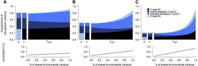
Finally, this concept of biased associations in covariate adjusted analysis can be extended to other effect measures. In particular, the heritability of a phenotype adjusted for a covariate, commonly reported,^22–26 can also be biased by the genetic component of the covariate and therefore might not necessarily represent the genetic component of the primary outcome. Similarly cross-trait heritability or genetic correlations between covariate adjusted phenotypes, as measured by Lee et al.,²⁷ might also be biased. Assuming an extended model from Figure 1D, the genetic component of the adjusted trait would correspond to a heterogeneous mixture of trait-specific genetic loci and shared loci with either effect in the same direction or effect in opposite direction (Figure 3). In theory, one can expect the heritability of an adjusted trait to be larger than the heritability of the unadjusted trait (Figure 3C). Cross-trait heritability estimates would provide a more comprehensive answer to the genetic variance overlap between correlated traits, although it is unclear how genetic effects in opposite direction for positively correlated traits (or conversely) are handled by these methods.

Figure 3.

Heritability of Adjusted Phenotypes

We compared the heritability of a given phenotype against the heritability estimated after adjustment for a correlated variable. We simulated a trait Y adjusted for a correlated trait C. The genetic variance of each trait (upper panel) splits into trait-specific effects, shared effects, and shared loci with opposite effects. We vary heritability of Y and C from 0.8 (A), 0.5 (B), and 0.2 (C) and the proportion of shared environmental variance (bottom panel) from 0 to 1.

Overall, when the goal is to identify genetic variants that are directly associated with a primary outcome, we were unable to identify an alternative approach that adjusts for a covariate and leads to unbiased effect estimates for a heritable covariate that is associated with the tested variant (see Appendix D). Therefore, unless we know with certainty that the tested variant does not influence the covariate, we recommend that the inclusion of such heritable covariates in the model should be avoided. Given evidence for a large number of pleiotropic genes across complex traits,^28–30 it seems unlikely that any heritable covariates with a complex genetic architecture, e.g., BMI or WHR, will fulfill that condition. Including such covariates in the absence of a strong prior knowledge on the pathophysiology is therefore likely to lead to biased effect estimates.

In some instances, the aim of an adjusted analysis is to increase statistical power rather than detect unbiased direct effects. In these instances, we suggest using multivariate approaches^31–33 that do not assume a causal diagram. Such approaches are generally well powered to detect pleiotropic loci affecting multiple traits, which are exactly the type of loci where we might expect the most power gain from adjusted analysis. However, if adjusted analyses are performed, we recommend reporting genetic effect estimates on the covariate and the outcome before and after the adjustment, their SD and significance, as well as the correlation between the outcome and the covariate. With this information in hand, the magnitude of a potential bias can be estimated and taken into account when interpreting the results.

Appendix A

Model

For simplicity we assume a linear model instead of a logistic model, which is often used for GWAS of case-control disease traits. However, the least-square estimates from a linear regression are a scaled first-order approximate of the log-odds obtained from a logistic regression.⁴ Therefore, given sufficient sample size, the issue highlighted in this letter also holds for case-control datasets when analyzed with logistic regression. Following the notation described in Figure 1, we can write the true causal model for the covariate C and the outcome Y as C = β_Cg + u_C, and Y = β_Yg + u_Y, where u_C and u_Y denote the combined contribution due to other loci, as well as the respective environmental (and noise) components of the covariate and the outcome. Note that this model does not rule out a direct contribution from C on Y (or vice versa), which could be included in the u_C and u_Y terms, respectively. However, such an effect could affect the interpretation of the direct effect estimates mentioned here (see Appendix B). If we assume that the covariate, the outcome, and the genotype have all been normalized to have mean zero and variance one, then we can write the marginal estimates for the genetic effects as ${\hat{\beta }}_Y=g^{\prime }Y/n$, and ${\hat{\beta }}_C=g^{\prime }C/n$, where n is the sample size. Similarly, the correlation coefficient can be written as ${\hat{\rho }}_{CY}=C^{\prime }Y/n$. Finally, we can write the adjusted model as Y = αC + β_Yadjg + ϵ, where α denotes the effect of C on Y, β_Yadj the genetic effect, and ϵ the environment (noise) term. Note that we do not believe that this is the generative model, rather the model that is being employed when performing GWAS on covariate adjusted outcomes.

Bias of the Effect Estimates in the Covariate Adjusted Model

From the adjusted model above we derived a joint least square estimates for the effect of C and g on Y, i.e., $\hat{\mathbf{\beta }}=\left[\begin{array}{c}\hat{\alpha }\\ {\hat{\beta }}_{Yadj}\end{array}\right]$, which can be written as $\hat{\mathbf{\beta }}={\left({\mathbf{X}}^{\prime }\mathbf{X}\right)}^{-1}{\mathbf{X}}^{\prime }\mathbf{y}$, where X is a matrix composed of c and g, the realization of C and g in a sample of n individuals, and y is a vector of realization of Y in the same sample. When C, Y and g are normally distributed with mean 0 and variance 1, $\hat{\mathbf{\beta }}$ can be re-written as

$$\hat{\mathbf{\beta }}={\left({\left[\mathbf{c},\mathbf{g}\right]}^{\text{'}}\left[\mathbf{c},\mathbf{g}\right]\right)}^{-1}{\left[\mathbf{c},\mathbf{g}\right]}^{\text{'}}\mathbf{y}$$

$$\hat{\mathbf{\beta }}={\left[\begin{array}{cc}{\mathbf{c}}^{\prime }\mathbf{c}& {\mathbf{c}}^{\prime }\mathbf{g}\\ {\mathbf{g}}^{\prime }\mathbf{c}& {\mathbf{g}}^{\prime }\mathbf{g}\end{array}\right]}^{-1}{\left[\mathbf{c},\mathbf{g}\right]}^{\prime }\mathbf{y}$$

$$\hat{\mathbf{\beta }}={\left[\begin{array}{cc}n& n{\hat{\beta }}_C\\ n{\hat{\beta }}_C& n\end{array}\right]}^{-1}{\left[\mathbf{c},\mathbf{g}\right]}^{\prime }\mathbf{y}$$

$$\hat{\mathbf{\beta }}=\frac{1}{n^2-n^2{\hat{\beta }}_C^2}\left[\begin{array}{cc}n& -n{\hat{\beta }}_C\\ -n{\hat{\beta }}_C& n\end{array}\right]{\left[\mathbf{c},\mathbf{g}\right]}^{\prime }\mathbf{y}$$

$$\hat{\mathbf{\beta }}=\frac{1}{n-n{\hat{\beta }}_C^2}{\left[\mathbf{c}-{\hat{\beta }}_C\mathbf{g},-{\hat{\beta }}_C\mathbf{c}+\mathbf{g}\right]}^{\prime }\mathbf{y}$$

$$\hat{\mathbf{\beta }}=\left[\begin{array}{c}\frac{1}{n-n{\hat{\beta }}_C^2}{\left(\mathbf{c}-{\hat{\beta }}_C\mathbf{g}\right)}^{\prime }\mathbf{y}\\ \frac{1}{n-n{\hat{\beta }}_C^2}{\left(-{\hat{\beta }}_C\mathbf{c}+\mathbf{g}\right)}^{\prime }\mathbf{y}\end{array}\right]$$

$$\hat{\mathbf{\beta }}=\left[\begin{array}{c}\frac{1}{n-n{\hat{\beta }}_C^2}\left({\mathbf{c}}^{\prime }\mathbf{y}-{\hat{\beta }}_C\mathbf{g}{}^{\prime }\mathbf{y}\right)\\ \frac{1}{n-n{\hat{\beta }}_C^2}\left(-{\hat{\beta }}_C{\mathbf{c}}^{\prime }\mathbf{y}+\mathbf{g}{}^{\prime }\mathit{y}\right)\end{array}\right]$$

$$\hat{\mathbf{\beta }}=\left[\begin{array}{c}\frac{1}{n-n{\hat{\beta }}_C^2}\left(n{\hat{\rho }}_{CY}-{\hat{\beta }}_{C}n{\hat{\beta }}_Y\right)\\ \frac{1}{n-n{\hat{\beta }}_C^2}\left(-{\hat{\beta }}_{C}n{\hat{\rho }}_{CY}+n{\hat{\beta }}_Y\right)\end{array}\right]$$

$$\hat{\mathbf{\beta }}=\left[\begin{array}{c}\frac{1}{1-{\hat{\beta }}_C^2}\left({\hat{\rho }}_{CY}-{\hat{\beta }}_C{\hat{\beta }}_Y\right)\\ \frac{1}{1-{\hat{\beta }}_C^2}\left(-{\hat{\beta }}_C{\hat{\rho }}_{CY}+{\hat{\beta }}_Y\right)\end{array}\right].$$

Assuming ${\hat{\beta }}_C^2\ll 1$, which is expected for most human phenotypes, including BMI, WHR, and WC the estimated effect of g can be approximated by ${\hat{\beta }}_{Yadj}\approx -{\hat{\beta }}_C{\hat{\rho }}_{CY}+{\hat{\beta }}_Y$. And therefore for a sample size n the expected value of ${\hat{\beta }}_{Yadj}$ can be approximated by

$$\text{E}\left({\hat{\beta }}_{Yadj}\right)\approx \text{E}\left(-{\hat{\beta }}_C{\hat{\rho }}_{CY}+{\hat{\beta }}_Y\right)\approx \text{E}\left(-{\hat{\beta }}_C{\hat{\rho }}_{CY}\right)+\text{E}\left({\hat{\beta }}_Y\right)\approx -{\beta }_C\times {\rho }_{CY}+cov\left({\hat{\beta }}_C,{\hat{\rho }}_{CY}\right)+{\beta }_Y.$$

Since ${\hat{\rho }}_{CY}=cor\left(C,Y\right)=cor\left({\hat{\beta }}_{C}g+{\epsilon }_C,{\hat{\beta }}_{Y}g+{\epsilon }_Y\right)={\hat{\beta }}_C{\hat{\beta }}_Y+{\gamma }_{res}$, where γ_res is the correlation between C and Y not explained by the SNP in the data, $\text{E}\left({\hat{\beta }}_{Yadj}\right)$ can be re-written as

$$\text{E}\left({\hat{\beta }}_{Yadj}\right)\approx -{\beta }_C\times {\rho }_{CY}+cov\left({\hat{\beta }}_C,{\hat{\beta }}_C{\hat{\beta }}_Y+{\gamma }_{res}\right)+{\beta }_Y$$

$$\text{E}\left({\hat{\beta }}_{Yadj}\right)\approx -{\beta }_C\times {\rho }_{CY}+cov\left({\hat{\beta }}_C,{\hat{\beta }}_C{\hat{\beta }}_Y\right)+{\beta }_Y$$

$$\text{E}\left({\hat{\beta }}_{Yadj}\right)\approx -{\beta }_C\times {\rho }_{CY}+{\sigma }_{{\hat{\beta }}_C}^2\times \text{E}\left({\hat{\beta }}_Y\right)+{\beta }_Y$$

$$\text{E}\left({\hat{\beta }}_{Yadj}\right)\approx -{\beta }_C\times {\rho }_{CY}+\frac{{\beta }_Y}{n}+{\beta }_Y.$$

For large sample size (e.g., n > 1000), $\text{E}\left({\hat{\beta }}_{Yadj}\right)$ can thus be approximated by β_Y −β_C × ρ_CY. It implies that $\text{E}\left({\hat{\beta }}_{Yadj}\right)\approx {\beta }_Y$ when β_C = 0, and is therefore unbiased; however, when β_C ≠ 0, using C as a covariate when testing the effect of G on Y introduce a bias approximately equal to −β_C × ρ_CY, which depends on the marginal effect of the genetic variant on the covariate and the correlation coefficient between the covariate and the outcome.

Finally, one can note that ${\hat{\rho }}_{CY}$ cannot be null when both ${\hat{\beta }}_Y$ and ${\hat{\beta }}_C$ are not null. Hence in the special case where ${\hat{\rho }}_{CY}$ is only explained by the shared genetic effect of g on Y and C, ${\hat{\rho }}_{CY}$ equals ${\hat{\rho }}_{CY}=cor\left(C,Y\right)=cor\left({\hat{\beta }}_{C}g+{\epsilon }_C,{\hat{\beta }}_{Y}g+{\epsilon }_Y\right)$, where ε_C and ε_Y are independent residual normally distributed with mean 0 and variance $\left(1-{\hat{\beta }}_C^2\right)$ and $\left(1-{\hat{\beta }}_Y^2\right),$ respectively. It follows that

$${\hat{\rho }}_{CY}={\hat{\beta }}_C\times {\hat{\beta }}_Y\times cor\left(g,g\right)+{\hat{\beta }}_C\times cor\left(g,{\epsilon }_Y\right)+{\hat{\beta }}_Y\times cor\left(g,{\epsilon }_C\right)+cor\left({\epsilon }_Y,{\epsilon }_C\right)={\hat{\beta }}_C\times {\hat{\beta }}_Y.$$

In such case the joint estimates becomes $\hat{\mathbf{\beta }}=\left[\begin{array}{c}0\\ \frac{1}{1-{\hat{\beta }}_C^2}\left({\hat{\beta }}_Y-{\hat{\beta }}_C^2{\hat{\beta }}_Y\right)\end{array}\right]=\left[\begin{array}{c}0\\ {\hat{\beta }}_Y\end{array}\right]$ and the estimated effects of g on Y before and after adjusting for C are equal.

Testing for a Bias in the Covariate Adjusted Analysis

Given the joint least-square estimates above, we can now write out their conditional distributions and make use of them to test different hypothesis. The hypothesis of interest is to test whether the observed association in the covariate adjusted model is expected when there is no direct genetic effect on C. In light of the equations above, a simple test for the bias is a test for a marginal association between the genetic variant and C, i.e., a test for β_C = 0. However, if we are unable to perform the marginal test, or if the reported values are calculated using a different sample, we can approximate the marginal test using only GWAS summary statistics ${\hat{\beta }}_{Yadj}$, ${\hat{\beta }}_Y$, and the reported correlation ${\hat{\rho }}_{CY}$. In particular, we are interested in the distribution of the joint least square estimate for the genotype effect in the covariate adjusted model under the null (β_C = 0). We can treat ${\hat{\beta }}_Y$ as an observed value, and get $E\left({\hat{\beta }}_{Yadj}|{\beta }_C=0,{\hat{\beta }}_Y={\hat{\beta }}_Y,{\hat{\rho }}_{CY}={\hat{\rho }}_{CY}\right)={\hat{\beta }}_Y$ and its variance, which equals

$$Var\left({\hat{\beta }}_{Yadj}|{\beta }_C=0,{\hat{\beta }}_Y={\hat{\beta }}_Y,{\hat{\rho }}_{CY}={\hat{\rho }}_{CY}\right)=Var\left(\frac{1}{1-{\hat{\beta }}_C^2}\text{|}{\beta }_C=0,{\hat{\beta }}_Y,{\hat{\rho }}_{CY}\right)\times Var\left({\hat{\beta }}_Y-{\hat{\beta }}_C{\hat{\rho }}_{CY}|{\beta }_C=0,{\hat{\beta }}_Y,{\hat{\rho }}_{CY}\right)+Var\left(\frac{1}{1-{\hat{\beta }}_C^2}\text{|}{\beta }_C=0,{\hat{\beta }}_Y,{\hat{\rho }}_{CY}\right)\times {\left(E\left({\hat{\beta }}_Y-{\hat{\beta }}_C{\hat{\rho }}_{CY}|{\beta }_C=0,{\hat{\beta }}_Y,{\hat{\rho }}_{CY}\right)\right)}^2+Var\left({\hat{\beta }}_Y-{\hat{\beta }}_C{\hat{\rho }}_{CY}|{\beta }_C=0,{\hat{\beta }}_Y,{\hat{\rho }}_{CY}\right)\times {\left(E\left(\frac{1}{1-{\hat{\beta }}_C^2}\text{|}{\beta }_C=0,{\hat{\beta }}_Y,{\hat{\rho }}_{CY}\right)\right)}^2.$$

Because $Var\left({\hat{\beta }}_Y-{\hat{\beta }}_C{\hat{\rho }}_{CY}|{\beta }_C=0,{\hat{\beta }}_Y,{\hat{\rho }}_{CY}\right)=Var\left({\hat{\beta }}_C{\hat{\rho }}_{CY}\text{|}{\beta }_C=0,{\hat{\rho }}_{CY}\right)={\hat{\rho }}_{CY}^2/n$ and $Var\left(1/1-{\hat{\beta }}_C^2\text{|}{\beta }_C=0,{\hat{\beta }}_Y,{\hat{\rho }}_{CY}\right)=Var\left(1/1-{\hat{\beta }}_C^2\text{|}{\beta }_C=0\right)\approx 0$ and $E\left(1/1-{\hat{\beta }}_C^2\text{|}{\beta }_C=0\right)\approx 1$ when sample size n is large, we have

$$Var\left({\hat{\beta }}_{Yadj}|{\beta }_C=0,{\hat{\beta }}_Y,{\hat{\rho }}_{CY}\right)=Var\left(\frac{1}{1-{\hat{\beta }}_C^2}\text{|}{\beta }_C=0\right)\times \frac{{\hat{\rho }}_{CY}^2}{n}+Var\left(\frac{1}{1-{\hat{\beta }}_C^2}\text{|}{\beta }_C=0\right)\times {\hat{\beta }}_Y^2+\frac{{\hat{\rho }}_{CY}^2}{n}\times {\left(E\left(\frac{1}{1-{\hat{\beta }}_C^2}\text{|}{\beta }_C=0\right)\right)}^2$$

$$Var\left({\hat{\beta }}_{Yadj}|{\beta }_C=0,{\hat{\beta }}_Y,{\hat{\rho }}_{CY}\right)=\approx \frac{{\hat{\rho }}_{CY}^2}{n}.$$

Using simulations, we verified that this is a very good approximation of the variance for realistic sample sizes, i.e., n > 1,000 (see Figure 2). Now that we have the mean and the variance conditional on β_C = 0, we can use a Wald test to test for a bias, i.e., test whether β_C ≠ 0. The Wald test statistic then becomes $n{\left({\hat{\beta }}_{Yadj}-{\hat{\beta }}_Y\right)}^2/{\hat{\rho }}_{CY}^2$. This test only requires the reported GWAS summary statistics, i.e., ${\hat{\beta }}_{Yadj}$, ${\hat{\beta }}_Y$, the reported correlation ${\hat{\rho }}_{CY}$, but not the marginal in-sample effect estimate ${\hat{\beta }}_C$. Since in-sample correlation estimates, ${\hat{\rho }}_{CY}^2$, may not be available there is a risk that the statistic is mis-calibrated by a constant factor where small values of ${\hat{\rho }}_{CY}^2$ can lead to false positives.

One can also note that the non-centrality parameter (ncp) of the above Wald test can be expressed as $ncp=\frac{n{\left(\frac{\left(-{\hat{\beta }}_C\times {\hat{\rho }}_{CY}+{\hat{\beta }}_Y\right)-{\hat{\beta }}_Y}{1-{\hat{\beta }}_C^2}\right)}^2}{{\hat{\rho }}_{CY}^2}=\frac{n{\hat{\beta }}_C^2}{1-{\hat{\beta }}_C^2}$, which corresponds to the ncp of the association test between G on C in the same sample.

We also confirmed the validity of the proposed test by analyzing a real data of 15,949 individuals from three cohorts, the Nurse’s Health Study, the Health Professional Study and the Physicians’ Health Study. We performed a genome-wide meta-analysis of WHR, BMI, and WHR adjusted for BMI across 6,106,189 SNPs either genotyped or imputed using the 1,000 genome reference panel.³⁴ All analyses were adjusted for relevant covariates including age, gender and the top 5 principal component of the genotypes. This analysis confirmed first that the difference in the genetic effect estimates from the BMI-adjusted and non-adjusted analysis of WHR directly depends on the genetic effect estimate on BMI and the correlation between WHR and BMI. Indeed, after accounting for BMI and WHR variances, we observed that $\left({\hat{\beta }}_{Yadj}-{\hat{\beta }}_Y\right)\sim \left({\hat{\beta }}_C\times {\hat{\rho }}_{CY}\right)$. We further compared the chi-square statistics from the proposed test: ${\left({\hat{\beta }}_{Yadj}-{\hat{\beta }}_Y)/({\sigma }_{{\hat{\beta }}_Y}\times {\hat{\rho }}_{CY}\right)}^2$ with the chi-square of the test of SNPs on BMI ${\left({\hat{\beta }}_C/{\sigma }_{{\hat{\beta }}_C}\right)}^2$. We observed a correlation of 0.98 between the two chi-squares, thus confirming the validity of the proposed test.

Proportion of Genetic Component

We derived the proportion of variance of an adjusted trait by each genetic component of the primary outcome and the covariate used for adjustment. Assume two normally distributed traits Y and C with mean 0 and variance 1, that have common and specific environmental component E_s, E₁ and E₂ respectively, a shared genetic component with effect in the same direction G_s and in opposite direction G_o respectively, and trait-specific genetic components G₁ and G₂ for Y and C respectively, so that

$$Y=\sqrt{c}\times E_s+\sqrt{e}\times E_1+\sqrt{1-c-e}\times \left(\sqrt{g_s}\times G_s+\sqrt{g_o}\times G_o+\sqrt{1-g_s-g_o}\times G_1\right)$$

$$C=\sqrt{c}\times E_s+\sqrt{e}\times E_2+\sqrt{1-c-e}\times \left(\sqrt{g_s}\times G_s-\sqrt{g_o}\times G_o+\sqrt{1-g_s-g_o}\times G_2\right)$$

The adjustment of Y for C is defined as Y_adjC = Y − αC where α, the correlation between the two traits equals c + (1 − c − e) ∗ (g_s − g_o). The proportion of variance of Y_adjC explained by each of the four genetic component is then

$$v_{G_s}=\left(1-c-e\right)\times g_s\times \frac{{\left(1-\alpha \right)}^2}{1-{\alpha }^2}$$

$$v_{G_o}=\left(1-c-e\right)\times g_o\times \frac{{\left(1+\alpha \right)}^2}{1-{\alpha }^2}$$

$$v_{G_1}=\left(1-c-e\right)\times \left(1-g_s-g_o\right)\times \frac{1}{1-{\alpha }^2}$$

$$v_{G_2}=\left(1-c-e\right)\times \left(1-g_s-g_o\right)\times \frac{{\alpha }^2}{1-{\alpha }^2}$$

Appendix B

Direct Acyclic Graphs and Interpretation of Adjusted Analysis

The use of causal diagrams or directed acyclic graphs (DAGs) in epidemiological research has been discussed in detail by many authors previously.^11–13,35 In this note, we summarize parts of their work that are relevant in the context of genetic epidemiology. The characterization of inter-relationships between the SNP (g), correlated trait (C), primary outcome (Y) and other relevant measured/unmeasured (U) variables with the help of causal diagrams or directed acyclic graphs (DAGs) can help understand whether an adjustment might be necessary (to avoid or reduce bias), unnecessary (increase variance of effect estimates), or harmful (lead to bias). We detail further 15 different DAGs (Figure S1) corresponding to four different scenarios where adjusting for a covariate is either recommended or should be avoided. We confirmed the validity of each through simulation (Table S3).

In general, when the exposure (in this case “g”) and the outcome share a common cause, adjustment for that variable (C, Figure S1A) or a surrogate of that variable (C is a surrogate for U, Figures S1B–S1D) is necessary.¹³ This adjustment can remove the confounding effect due to the common cause, although when the covariate is only a surrogate, it will not completely solve the confounding issue (Figure S1B and Table S3). Such a scenario is unlikely in genetic epidemiological studies, since very few factors precede the occurrence/acquisition of germline genetic variants. The main example of an upstream factor that influences genotype distribution is population stratification; adjustment for principal components can reduce the effects of population stratification bias. Therefore, it can be argued that in order to reduce confounding of the genetic effect on the primary outcome in genetic epidemiological studies, it is rarely necessary to adjust for anything more than principal components (adjustment for additional covariates in certain situations can increase power, however⁴).

Next, we consider a scenario where the effect of the G on Y is hypothesized to be completely or partially mediated through C, or equivalently when C is a surrogate for a mediator. Such a mediation is represented in causal diagrams by an indirect, unblocked path that goes through C, or through factors tagged by C (Figures S1E–S1H). Here, classical epidemiologists advise against adjustment for C, since C is in the causal pathway and hence not a confounder.^12,13 In contrast, instances can be found where genetic epidemiologists seek the controlled direct causal effect of G on Y by noting their intent to identify variants associated with the outcome without covariate mediation, and are thereby justified in adjusting for C, in the absence of an unmeasured confounder³⁶ described in the next paragraph. In Figures S1E–S1H, there are two paths from G to Y—a direct path and an indirect path that goes through C. Statistical models that condition for C block the path through C and reveal only the direct effect of G on Y. We also note that when the covariate is only a surrogate for the mediator, the interpretation can be difficult as the proportion of the “true” indirect path removed is unknown (Figure S1h and Table S3)

However, if an unmeasured variable U, not considered in the study, influences both C and Y, adjusting for C will result in the formation of a backdoor path from G to Y (Figures S1I and S1J). This path does not follow the direction of the arrows and is blocked at C. Whenever a path is blocked at a variable, that variable is termed a collider. Statistical models that condition for colliders (or their descendants) on a path from G to Y unblock that path, and can result in biased effect estimate of G on Y.^11,13 In a scenario where C and Y both influence a collider U (Figure S1K), because C is not a descendant of U, adjusting for C will not lead to bias, but is at the same time unnecessary.

Lastly, let us consider scenarios where, due to incomplete understanding of complex traits and unbeknownst to investigators, C is a descendant of Y (Figures S1L–S1O). In such a scenario, the indirect path from G to Y will be blocked, and adjustment for C could result in spurious associations due to opening of that backdoor path. One possible example of a study where the adjustment covariate might be the descendant of the primary outcome is the GWAS of pro-insulin levels adjusted for insulin—in biological pathways, insulin is produced from pro-insulin by removal of the C-peptide,³⁷ and hence insulin levels might be influenced by pro-insulin levels. Therefore, adjustment of insulin levels would not lead to identification of SNPs associated with pro-insulin alone, but some of the identified SNPs may be related to the downstream process of conversion from pro-insulin to insulin.

In summary, if an indirect path from G to Y is not blocked, adjustment for C on the path could be utilized to get an estimate of direct association between G and Y. On the other hand, if the indirect path between G and Y is blocked, adjustment for colliders (or their descendants) in the path could result in biased estimates. More complex scenarios might arise and might be resolved by applying principles described in previous literature.^11,13

Appendix C

Analysis of the GIANT Data

We considered for illustrative purpose the 23 SNPs reported to be associated at genome-wide significance levels in gender specific samples with waist hip ratio (WHR) and waist circumference (WC) after adjustment on body mass index (BMI) by Heid et al.⁶ and Randal et al.⁸ We extracted from the GIANT summary statistics database the estimated effects of those SNPs on WHR, or WC when relevant, before and after adjustment for BMI, and the marginal effect of those SNPs on BMI. All estimates were selected from the sex stratified anthropometrics analysis.⁸ The sample sizes (averaged over all SNPs) used for each of the 6 analyses were as follows: for BMI, there were 52,239 and 60,575 subjects in the male and female analysis respectively; for WHR, there were 30,713 and 38,016; for WHR adjusted for BMI, there were 30,715 and 38,028; for WC, there were 33,989 and 42,060; and for WC adjusted for BMI, there were 34,059 and 42,226. We derived the correlation between BMI and WHR and WC in males and females from Table S8 of Heid et al.⁶ using a sample size weighted average. We obtained the following correlation: cor(BMI,WHR)_female = 0.42, cor(BMI,WHR)_male = 0.56, cor(BMI,WC)_female = 0.84, cor(BMI,WC)_male = 0.86.

We noted that the majority of the SNPs (78%) had effects in opposite direction for BMI and WHR/WC. We confirmed through simulation that the expected proportion of SNPs having effect in opposite direction in a model where the genetic variant is associated with the outcome, but not the covariate, is smaller or equal to 50%. When two traits are positively correlated and neither is associated with the SNPs tested, the two sets of estimates (on BMI and WHR/WC in this case) are also expected to be positively correlated (Figure S3A), and therefore most SNPs should display effects in the same direction, i.e., the fraction of SNPs with effects in the same direction will be >0.5. In the presence of a true association between the SNP and the outcome, this fraction decreases toward 0.5 (Figure S3B). Using this lower, conservative expected fraction of 0.5, the probability that the fraction SNPs with opposite effects is equal to or greater than the observed fraction of 78% is p = 5 × 10⁻³. These simulations also show that the potential presence of an opposite effect due to chance (i.e., β_C = 0 but ${\hat{\beta }}_C\ne 0$) would not impact power in adjusted analysis. The intuition is that positive correlation between the outcome and the covariate implies that the estimates ${\hat{\beta }}_C$ and ${\hat{\beta }}_Y$ follow the same pattern, i.e., when ${\hat{\beta }}_C$ is smaller than zero, ${\hat{\beta }}_Y$ tend to be smaller than β_Y and conversely. Therefore, the adjusted estimate ${\hat{\beta }}_{Yadj}$ which approximately equals ${\hat{\beta }}_Y-{\hat{\beta }}_C{\hat{\rho }}_{CY}$ tends to change toward the true estimate. Hence the p-value for ${\hat{\beta }}_{Yadj}$ is not influenced by ${\hat{\beta }}_C$ when β_C = 0 (Figure S3, lower panel).

Appendix D

Evaluation of Alternatives Approaches

This study and previous works (see Appendix B) showed that variables that shared causal factors with the outcome should not be used for adjustment purposes. We explored two potential solutions in a GWAS context to address situation where β_C ≠ 0. One first solution consists in using C_adj.g, the residual of C adjusted for the effect of g. Because the genetic effect is removed from the C, adjusting the primary outcome Y for C_adj.g would a priori not induce bias. However, the problem of deriving this residual is that it depends on the accuracy of ${\hat{\beta }}_C$, the estimate of the effect of G on C, which will be accurate for infinite sample size but noisy for small sample size. Hence, while adjusting C for the true effect of g removes the bias, a “residual bias” remains when using the estimated C_adj.g (Figure S5). When applied on a GWAS scale, it can actually introduce more bias that the standard adjustment. As the vast majority of the SNPs are expected to be under the null, using C_adj.g as a covariate can potentially introduce bias in all tests. Second, we considered a stratified approach, where the genetic effect on the primary outcome is evaluated in strata defined by the covariate. Using the same simulation scheme, we tested the marginal association between g and Y independently in subjects with high versus low values for C. As in the previous analysis, such a strategy does not solve the bias issue (Figure S5). The intuition here is that individuals with large values of C also display large values for Y and g when both are positively correlated with C (and conversely). Hence removing those subjects induces a negative correlation between Y and g (Figure S6). Overall we did not identify any general solution to this issue in the literature. However, for the very specific case where the latent variables that explain the correlation between the C and Y have been measured, some proposed a two-steps adjustment procedure that might correct for the bias.¹⁴ Although this approach might be relevant for that specific scenario, whenever the latent variables are unmeasured—as assumed in this study—the proposed two-step approach does not solve the issue (Figure S5).

Web Resources

The URLs for data presented herein are as follows:

• GIANT consortium data files, http://www.broadinstitute.org/collaboration/giant

• OMIM, http://www.omim.org/

References

- 1.Price A.L., Patterson N.J., Plenge R.M., Weinblatt M.E., Shadick N.A., Reich D. Principal components analysis corrects for stratification in genome-wide association studies. Nat. Genet. 2006;38:904–909. doi: 10.1038/ng1847. [DOI] [PubMed] [Google Scholar]
- 2.Pickrell J.K., Marioni J.C., Pai A.A., Degner J.F., Engelhardt B.E., Nkadori E., Veyrieras J.B., Stephens M., Gilad Y., Pritchard J.K. Understanding mechanisms underlying human gene expression variation with RNA sequencing. Nature. 2010;464:768–772. doi: 10.1038/nature08872. [DOI] [PMC free article] [PubMed] [Google Scholar]
- 3.Mefford J., Witte J.S. The Covariate’s Dilemma. PLoS Genet. 2012;8:e1003096. doi: 10.1371/journal.pgen.1003096. [DOI] [PMC free article] [PubMed] [Google Scholar]
- 4.Pirinen M., Donnelly P., Spencer C. Efficient computation with a linear mixed model on large-scale data sets with applications to genetic studies. Ann. Appl. Stat. 2013;7:369–390. [Google Scholar]
- 5.Kaplan R.C., Petersen A.K., Chen M.H., Teumer A., Glazer N.L., Döring A., Lam C.S., Friedrich N., Newman A., Müller M. A genome-wide association study identifies novel loci associated with circulating IGF-I and IGFBP-3. Hum. Mol. Genet. 2011;20:1241–1251. doi: 10.1093/hmg/ddq560. [DOI] [PMC free article] [PubMed] [Google Scholar]
- 6.Heid I.M., Jackson A.U., Randall J.C., Winkler T.W., Qi L., Steinthorsdottir V., Thorleifsson G., Zillikens M.C., Speliotes E.K., Mägi R., MAGIC Meta-analysis identifies 13 new loci associated with waist-hip ratio and reveals sexual dimorphism in the genetic basis of fat distribution. Nat. Genet. 2010;42:949–960. doi: 10.1038/ng.685. [DOI] [PMC free article] [PubMed] [Google Scholar]
- 7.Manning A.K., Hivert M.F., Scott R.A., Grimsby J.L., Bouatia-Naji N., Chen H., Rybin D., Liu C.T., Bielak L.F., Prokopenko I., DIAbetes Genetics Replication And Meta-analysis (DIAGRAM) Consortium. Multiple Tissue Human Expression Resource (MUTHER) Consortium A genome-wide approach accounting for body mass index identifies genetic variants influencing fasting glycemic traits and insulin resistance. Nat. Genet. 2012;44:659–669. doi: 10.1038/ng.2274. [DOI] [PMC free article] [PubMed] [Google Scholar]
- 8.Randall J.C., Winkler T.W., Kutalik Z., Berndt S.I., Jackson A.U., Monda K.L., Kilpeläinen T.O., Esko T., Mägi R., Li S., DIAGRAM Consortium. MAGIC Investigators Sex-stratified genome-wide association studies including 270,000 individuals show sexual dimorphism in genetic loci for anthropometric traits. PLoS Genet. 2013;9:e1003500. doi: 10.1371/journal.pgen.1003500. [DOI] [PMC free article] [PubMed] [Google Scholar]
- 9.Scott R.A., Lagou V., Welch R.P., Wheeler E., Montasser M.E., Luan J., Mägi R., Strawbridge R.J., Rehnberg E., Gustafsson S., DIAbetes Genetics Replication and Meta-analysis (DIAGRAM) Consortium Large-scale association analyses identify new loci influencing glycemic traits and provide insight into the underlying biological pathways. Nat. Genet. 2012;44:991–1005. doi: 10.1038/ng.2385. [DOI] [PMC free article] [PubMed] [Google Scholar]
- 10.Pearl J. Causal inference from indirect experiments. Artif. Intell. Med. 1995;7:561–582. doi: 10.1016/0933-3657(95)00027-3. [DOI] [PubMed] [Google Scholar]
- 11.Greenland S., Pearl J., Robins J.M. Causal diagrams for epidemiologic research. Epidemiology. 1999;10:37–48. [PubMed] [Google Scholar]
- 12.Schisterman E.F., Cole S.R., Platt R.W. Overadjustment bias and unnecessary adjustment in epidemiologic studies. Epidemiology. 2009;20:488–495. doi: 10.1097/EDE.0b013e3181a819a1. [DOI] [PMC free article] [PubMed] [Google Scholar]
- 13.Hernán M.A., Hernández-Díaz S., Werler M.M., Mitchell A.A. Causal knowledge as a prerequisite for confounding evaluation: an application to birth defects epidemiology. Am. J. Epidemiol. 2002;155:176–184. doi: 10.1093/aje/155.2.176. [DOI] [PubMed] [Google Scholar]
- 14.Vansteelandt S., Goetgeluk S., Lutz S., Waldman I., Lyon H., Schadt E.E., Weiss S.T., Lange C. On the adjustment for covariates in genetic association analysis: a novel, simple principle to infer direct causal effects. Genet. Epidemiol. 2009;33:394–405. doi: 10.1002/gepi.20393. [DOI] [PMC free article] [PubMed] [Google Scholar]
- 15.Juul A., Dalgaard P., Blum W.F., Bang P., Hall K., Michaelsen K.F., Müller J., Skakkebaek N.E. Serum levels of insulin-like growth factor (IGF)-binding protein-3 (IGFBP-3) in healthy infants, children, and adolescents: the relation to IGF-I, IGF-II, IGFBP-1, IGFBP-2, age, sex, body mass index, and pubertal maturation. J. Clin. Endocrinol. Metab. 1995;80:2534–2542. doi: 10.1210/jcem.80.8.7543116. [DOI] [PubMed] [Google Scholar]
- 16.Chan J.M., Stampfer M.J., Ma J., Gann P., Gaziano J.M., Pollak M., Giovannucci E. Insulin-like growth factor-I (IGF-I) and IGF binding protein-3 as predictors of advanced-stage prostate cancer. J. Natl. Cancer Inst. 2002;94:1099–1106. doi: 10.1093/jnci/94.14.1099. [DOI] [PubMed] [Google Scholar]
- 17.Thorleifsson G., Walters G.B., Gudbjartsson D.F., Steinthorsdottir V., Sulem P., Helgadottir A., Styrkarsdottir U., Gretarsdottir S., Thorlacius S., Jonsdottir I. Genome-wide association yields new sequence variants at seven loci that associate with measures of obesity. Nat. Genet. 2009;41:18–24. doi: 10.1038/ng.274. [DOI] [PubMed] [Google Scholar]
- 18.Zaitlen N., Lindström S., Pasaniuc B., Cornelis M., Genovese G., Pollack S., Barton A., Bickeböller H., Bowden D.W., Eyre S. Informed conditioning on clinical covariates increases power in case-control association studies. PLoS Genet. 2012;8:e1003032. doi: 10.1371/journal.pgen.1003032. [DOI] [PMC free article] [PubMed] [Google Scholar]
- 19.Stergiakouli E., Gaillard R., Tavare J.M., Balthasar N., Loos R.J., Taal H.R., Evans D.M., Rivadeneira F., St Pourcain B., Uitterlinden A.G. Genome-wide association study of height-adjusted BMI in childhood identifies functional variant in ADCY3. Obesity. 2014;22:2252–2259. doi: 10.1002/oby.20840. [DOI] [PMC free article] [PubMed] [Google Scholar]
- 20.Loth D.W., Artigas M.S., Gharib S.A., Wain L.V., Franceschini N., Koch B., Pottinger T.D., Smith A.V., Duan Q., Oldmeadow C. Genome-wide association analysis identifies six new loci associated with forced vital capacity. Nat. Genet. 2014;46:669–677. doi: 10.1038/ng.3011. [DOI] [PMC free article] [PubMed] [Google Scholar]
- 21.Hancock D.B., Eijgelsheim M., Wilk J.B., Gharib S.A., Loehr L.R., Marciante K.D., Franceschini N., van Durme Y.M., Chen T.H., Barr R.G. Meta-analyses of genome-wide association studies identify multiple loci associated with pulmonary function. Nat. Genet. 2010;42:45–52. doi: 10.1038/ng.500. [DOI] [PMC free article] [PubMed] [Google Scholar]
- 22.Mills G.W., Avery P.J., McCarthy M.I., Hattersley A.T., Levy J.C., Hitman G.A., Sampson M., Walker M. Heritability estimates for beta cell function and features of the insulin resistance syndrome in UK families with an increased susceptibility to type 2 diabetes. Diabetologia. 2004;47:732–738. doi: 10.1007/s00125-004-1338-2. [DOI] [PubMed] [Google Scholar]
- 23.Stein C.M., Guwatudde D., Nakakeeto M., Peters P., Elston R.C., Tiwari H.K., Mugerwa R., Whalen C.C. Heritability analysis of cytokines as intermediate phenotypes of tuberculosis. J. Infect. Dis. 2003;187:1679–1685. doi: 10.1086/375249. [DOI] [PMC free article] [PubMed] [Google Scholar]
- 24.Post W.S., Larson M.G., Myers R.H., Galderisi M., Levy D. Heritability of left ventricular mass: the Framingham Heart Study. Hypertension. 1997;30:1025–1028. doi: 10.1161/01.hyp.30.5.1025. [DOI] [PubMed] [Google Scholar]
- 25.Murabito J.M., Guo C.Y., Fox C.S., D’Agostino R.B. Heritability of the ankle-brachial index: the Framingham Offspring study. Am. J. Epidemiol. 2006;164:963–968. doi: 10.1093/aje/kwj295. [DOI] [PubMed] [Google Scholar]
- 26.Shah S.H., Hauser E.R., Bain J.R., Muehlbauer M.J., Haynes C., Stevens R.D., Wenner B.R., Dowdy Z.E., Granger C.B., Ginsburg G.S. High heritability of metabolomic profiles in families burdened with premature cardiovascular disease. Mol. Syst. Biol. 2009;5:258. doi: 10.1038/msb.2009.11. [DOI] [PMC free article] [PubMed] [Google Scholar]
- 27.Lee S.H., Ripke S., Neale B.M., Faraone S.V., Purcell S.M., Perlis R.H., Mowry B.J., Thapar A., Goddard M.E., Witte J.S., Cross-Disorder Group of the Psychiatric Genomics Consortium. International Inflammatory Bowel Disease Genetics Consortium (IIBDGC) Genetic relationship between five psychiatric disorders estimated from genome-wide SNPs. Nat. Genet. 2013;45:984–994. doi: 10.1038/ng.2711. [DOI] [PMC free article] [PubMed] [Google Scholar]
- 28.Cotsapas C., Voight B.F., Rossin E., Lage K., Neale B.M., Wallace C., Abecasis G.R., Barrett J.C., Behrens T., Cho J., FOCiS Network of Consortia Pervasive sharing of genetic effects in autoimmune disease. PLoS Genet. 2011;7:e1002254. doi: 10.1371/journal.pgen.1002254. [DOI] [PMC free article] [PubMed] [Google Scholar]
- 29.Sivakumaran S., Agakov F., Theodoratou E., Prendergast J.G., Zgaga L., Manolio T., Rudan I., McKeigue P., Wilson J.F., Campbell H. Abundant pleiotropy in human complex diseases and traits. Am. J. Hum. Genet. 2011;89:607–618. doi: 10.1016/j.ajhg.2011.10.004. [DOI] [PMC free article] [PubMed] [Google Scholar]
- 30.Andreassen O.A., Djurovic S., Thompson W.K., Schork A.J., Kendler K.S., O’Donovan M.C., Rujescu D., Werge T., van de Bunt M., Morris A.P., International Consortium for Blood Pressure GWAS. Diabetes Genetics Replication and Meta-analysis Consortium. Psychiatric Genomics Consortium Schizophrenia Working Group Improved detection of common variants associated with schizophrenia by leveraging pleiotropy with cardiovascular-disease risk factors. Am. J. Hum. Genet. 2013;92:197–209. doi: 10.1016/j.ajhg.2013.01.001. [DOI] [PMC free article] [PubMed] [Google Scholar]
- 31.Aschard H., Vilhjálmsson B.J., Greliche N., Morange P.E., Trégouët D.A., Kraft P. Maximizing the power of principal-component analysis of correlated phenotypes in genome-wide association studies. Am. J. Hum. Genet. 2014;94:662–676. doi: 10.1016/j.ajhg.2014.03.016. [DOI] [PMC free article] [PubMed] [Google Scholar]
- 32.Zhou X., Stephens M. Efficient multivariate linear mixed model algorithms for genome-wide association studies. Nat. Methods. 2014;11:407–409. doi: 10.1038/nmeth.2848. [DOI] [PMC free article] [PubMed] [Google Scholar]
- 33.Korte A., Vilhjálmsson B.J., Segura V., Platt A., Long Q., Nordborg M. A mixed-model approach for genome-wide association studies of correlated traits in structured populations. Nat. Genet. 2012;44:1066–1071. doi: 10.1038/ng.2376. [DOI] [PMC free article] [PubMed] [Google Scholar]
- 34.Abecasis G.R., Auton A., Brooks L.D., DePristo M.A., Durbin R.M., Handsaker R.E., Kang H.M., Marth G.T., McVean G.A., 1000 Genomes Project Consortium An integrated map of genetic variation from 1,092 human genomes. Nature. 2012;491:56–65. doi: 10.1038/nature11632. [DOI] [PMC free article] [PubMed] [Google Scholar]
- 35.Rothman K.J., Greenland S., Lash T.L. Lippincott, Williams & Wilkins; Philadelphia, PA: 2008. Modern Epidemiology. [Google Scholar]
- 36.Cole S.R., Hernán M.A. Fallibility in estimating direct effects. Int. J. Epidemiol. 2002;31:163–165. doi: 10.1093/ije/31.1.163. [DOI] [PubMed] [Google Scholar]
- 37.Steiner D.F., Cunningham D., Spigelman L., Aten B. Insulin biosynthesis: evidence for a precursor. Science. 1967;157:697–700. doi: 10.1126/science.157.3789.697. [DOI] [PubMed] [Google Scholar]
Associated Data
This section collects any data citations, data availability statements, or supplementary materials included in this article.