

SUMMARY
In this article, we present a systematic comparison of computational hemodynamics in arterial models with deformable vessel walls using a one-dimensional (1-D) and a three-dimensional (3-D) method. The simulations were performed using a series of idealized compliant arterial models representing the common carotid artery, thoracic aorta, aortic bifurcation, and full aorta from the arch to the iliac bifurcation. The formulations share identical outflow boundary conditions and have compatible material laws. We also present an iterative algorithm to select the parameters for the outflow boundary conditions using the 1-D theory to achieve a desired systolic and diastolic pressure at a particular vessel. This 1-D/3-D framework can be used to efficiently determine material and boundary condition parameters for 3-D subject-specific arterial models with deformable vessel walls. Finally, we explore the impact of different anatomical features and hemodynamic conditions on the numerical predictions. The results show good agreement between the two schemes, especially during the diastolic phase of the cycle.
Keywords: Arterial Hemodynamics, Fluid Structure Interaction, Pulse Wave Propagation, Windkessel, Full Aorta Model, Spatially-Varying Mechanical Properties, Outflow Boundary Condition Estimation
1. INTRODUCTION
One-dimensional (1-D) and three-dimensional (3-D) formulations have been used extensively to simulate arterial hemodynamics. Landmark contributions in 1-D modeling include the works of Hughes and Lubliner [1], Stergiopulos et al. [2, 3], Olufsen et al. [4], Formaggia et al. [5], Sherwin et al. [6], Bessems et al. [7], Mynard and Nithiarasu [8], Alastruey et al. [9], and Müller and Toro [10]. Key contributions to 3-D blood flow modeling in deformable vessels include the works of Perktold et al. [11], Taylor et al. [12], Quarteroni et al. [13], Steinman et al. [14], Cebral et al. [15], Gerbeau et al. [16], and Figueroa et al. [17]. 1-D methods have been used to improve our theoretical understanding of hemodynamics, in particular to study the mechanisms underlying pulse wave propagation [18, 19] and also clinically in applications such as wave intensity analysis [20]. Accurate predictions can be made when when the flow is predominantly unidirectional and there are no sudden changes in cross-sectional area. However, 1-D models require the introduction of additional empirical laws to account for recirculation and pressure losses in the presence of vessel curvatures, stenoses, aneurysms, etc. [2, 21, 22] These geometric complexities are intrinsically captured with 3-D models, which can provide localized hemodynamic quantities such as wall shear stress, particle residence time, etc. Additionally, 3-D modeling enables the use of structurally-motivated biaxial constitutive laws [23] and circumferentially-varying mechanical properties for the arterial wall [24] and the simulation of complex processes such as the interactions between the arterial wall and medical devices [25, 26]. Nevertheless, 1-D models typically contain far fewer degrees of freedom in comparison to 3-D models (on the order of 103 versus 106) and the simulations can be executed in a matter of minutes on a personal laptop computer.
Previous works have compared 1-D models and 3-D models with rigid walls in the context of cerebral arterial flow [27, 28] and with deformable vessels in the aorta under steady flow [29]. However, a systematic comparison between 1-D and 3-D models in a variety of deformable arterial configurations was still missing in the literature. In general, a good agreement between the two modeling techniques is expected when the flow is mostly unidirectional and there are no sudden changes in cross-sectional area, while larger differences are expected in more complex configurations, such as in curved vessels and areas with highly dynamic flows. For a proper comparison to be made, a framework containing the 1-D and 3-D formulations that share equivalent boundary conditions and material laws must be developed. In general, this framework can be used to quickly estimate boundary condition parameters and distributions of material coefficients for an extensive multi-branched 3-D model (e.g. a full-body scale arterial network model [30]), a task that is more time-consuming in the isolated 3-D setting. The purpose of this paper is twofold:
To perform a systematic comparison between cross-sectionally-averaged hemodynamics (i.e. average flow, average pressure and radial deformation) obtained with two specific implementations of the 1-D and 3-D formulations in a series of four increasingly complex idealized geometries representing the common carotid artery, the thoracic aorta, the aortoilliac bifurcation and the full aorta including the first generation of branches. This simplified set of geometries, as opposed to patient-specific geometries, allows for a more direct comparison between the 1-D and 3-D schemes. We investigated the differences in the hemodynamic predictions introduced by increased Reynolds number, the presence of tapering, curvature, and bifurcation angles. To ensure a consistent comparison between formulations, we used equivalent constitutive laws in the 1-D and 3-D formulations, imposed identical flow waveforms and velocity profiles at the inlets, and coupled three-element Windkessel models at the outlets. In these comparisons, the 1-D geometric parameters were obtained directly using dimensions taken from the idealized 3-D geometries (see Fig. 1).
To develop a computational framework where a 1-D model is used to quickly determine boundary condition and material parameters to match patient data such as flow and pressure waveforms and localized measurements of distensibility. Once evaluated, the parameters are fed directly to the 3-D model to perform localized studies. Our aim is to exploit the advantages of both schemes: a computationally efficient 1-D model combined with a full 3-D model sharing identical boundary condition and constitutive laws. This overlapping 3-D/1-D approach can potentially accelerate the solution turn-around time of complex 3-D models, therefore improving their clinical applicability, and differs from previous efforts [13, 31, 32, 33] where 3-D and 1-D models were coupled to represent spatially distinct parts of the arterial tree.
Figure 1.

Schematic representation of the modeling approach adopted in this study: 1-D and 3-D models share common inflow and outflow boundary conditions, as well as compatible consitutive laws. The 1-D geometry is obtained from the centerlines of the 3-D model, and vessel diameters and wall thickness are identical.
The structure of this paper is as follows: we first present the details of the 1-D and 3-D formulations utilized in this work, paying special attention to the description of boundary conditions and material laws that are consistent between the two approaches. We then compare the numerical predictions of both methods in a series of idealized geometries. Finally, we describe and discuss the similarities and differences in the results between the two formulations and finish with conclusions and future work.
2. METHODS
2.1. One-dimensional Formulation
Conservation of mass and momentum applied to a 1-D impermeable and deformable tubular control volume of an incompressible Newtonian fluid yields [6, 34, 19]
| (1) |
where x is the axial coordinate along the vessel, t is the time, A(x, t) is the cross-sectional area of the lumen, U(x, t) is the axial blood flow velocity averaged over the cross-section, P(x, t) is the blood pressure averaged over the cross-section, ρf is the density of blood assumed to be constant and f(x, t) is the frictional force per unit length. The momentum correction factor in the convection acceleration term of Eq. (1) was assumed to be equal to one, following the work of Stergiopulos et al. [2]. Equation (1) can also be derived by integrating the incompressible Navier-Stokes equations over a generic cross section of a cylindrical domain [1, 35, 36, 37].
In this work, the velocity profile is assumed to be constant in shape and axisymmetric. The axial velocity (u) is assumed to have the shape
| (2) |
where r(x, t) is the lumen radius, ξ is the radial coordinate and ζ is the polynomial order. Following [35], ζ = 9 provides a good compromise fit to experimental data obtained at different points in the cardiac cycle.
Integration of the Navier-Stokes equations of an incompressible Newtonian fluid for axisymmetric vessels yields [35]. For the velocity profile given by Eq. (2) we have f = −2(ζ + 2) μπU in which the local f is proportional to the local flow. Note that ζ = 2 leads to the Poiseuille flow resistance f = −8μπU. For all of the simulations presented, μ = 4 mPa s and ρf = 1060 kg/m3.
An explicit algebraic relationship between P and A (or tube law) is also required to close Eq. (1) and account for the fluid-structure interaction of the problem. In general we have P =
 (A(x, t); x, t), where the function
depends on the model used to describe the dynamics of the arterial wall.
(A(x, t); x, t), where the function
depends on the model used to describe the dynamics of the arterial wall.
We solved Eqs. (1) with the elastic tube law described in Section 2.3 using a discontinuous Galerkin scheme with a spectral/hp spatial discretization and a second-order Adams-Bashforth time discretization [9]. The initial conditions are (A(x, 0), U(x, 0), P(x, 0)) = (A0(x), 0, 0), where A0 is the initial area that yields Ad at P = Pd, with Pd the diastolic pressure. In all our 1-D simulations we implemented boundary conditions and solved matching conditions at bifurcations by taking into account the correct propagation of the characteristic information and neglecting energy losses [19, 38].
2.2. Three-dimensional Formulation
The coupled-momentum method [17] is used to formulate the 3-D FSI problem. Here, the degrees of freedom for the vessel wall (displacements u) are described as a function of the fluid velocities at the fluid-wall interface, Σ, using an “enhanced” membrane formulation. Under the assumption of a fixed fluid domain, i.e. linearized kinematics of the vessel wall, the strong form is defined in an Eulerian configuration:
| (3) |
| (4) |
where Ωf denotes the fluid domain, v is the fluid velocity, p is the pressure, b is a body force (here, assumed to be zero), and τf = μ(∇v + (∇v)T) is the viscous stress tensor for a Newtonian fluid. The arterial wall is treated as a thin membrane with thickness h and density ρs where vs is the solid velocity, σs is the membrane stress tensor, and ns is the outward normal at the fluid-wall interface. The value of ρs was 0.001 g/mm3 for all models.
To account for the mechanical forces exerted by the external tissues on the arterial walls, an additional term, fsupport = (ksu + csv), was included in Eq. (4) which approximates the mechanical behavior of the external tissue [39], where the parameters ks and cs are the stiffness and damping coefficients. This additional force can be used to eliminate spurious and nonphysiological oscillations in specific cases where the geometry is elongated and the vessel wall experiences asymmetric loads. For the simulations presented in this paper, unless explicitly stated, the values of ks and cs are set to zero.
With the assumption that the vessel wall thickness (h) is small and with appropriate choices for the solution and test function spaces,
 ,
,
 and
and
 , the strong form gives rise to the variational equation:
| (5) |
where w ∈
and q ∈
are test functions. Γin is a Dirichlet boundary where the test functions w vanish and where the fluid velocities are prescribed, i.e. at the inlet. The traction term h(v, p) on the outlet boundary Γout is given as a function of v and p depending on the reduced-order model (i.e. three-element Windkessel) chosen to represent the downstream vasculature, as described by Vignon-Clementel et al. [40, 41]. The augmented Lagrangian scheme described by Kimet al. [42] was used to stabilize the outflow velocities in the presence of flow reversal at the outflow boundaries.
To discretize and solve Eq. (5), we employed a stabilized semi-discrete finite element method based on the work of Brooks and Hughes [43], Franca and Frey [44], Taylor et al. [12], and Whiting and Jansen [45], using equal-order interpolation (P1/P1 elements) for the velocity and pressure fields. The generalized α-method [46, 47] was used to integrate the system of ordinary differential equations resulting from the finite element discretization.
2.3. Material Laws
The arterial wall was modeled as a thin, incompressible, homogeneous, isotropic, linear elastic membrane characterized by an elastic modulus E, a Poisson’s ratio ν = 0.5, and a thickness h.
In the 1-D model, the arterial wall is assumed to deform axisymmetrically, each cross-section independently of the others, so that the relationship between circumferential hoop stress, Tθ, and radial displacement is
| (6) |
where rd is the radius at diastolic pressure (Pd). Applying Laplace’s law, Tθ = (P − Pd)r/h, and assuming that 1/r can be approximated by 1/rd, we obtain the tube law [9]
| (7) |
where Ad(x) is the luminal area at diastolic pressure. In Eq. (7), both E and h are functions of the position x. The pulse wave speed c(x, t) is related to A through
| (8) |
The initial area A0 is calculated by replacing P = 0 and A = A0 in Eq. (7), which leads to
| (9) |
In the 3-D formulation, no assumptions regarding axisymmetry were made. The enhanced membrane stress tensor σs is given as a function of a tensor K̃ of material parameters, a tensor P̃ describing the pre-stress of the wall, and the infinitesimal strain tensor ε̃; σs = K̃ ε̃, with
| (10) |
| (11) |
where k is a transverse shear factor and u is the displacement vector [48]. In general, the pre-stress tensor can be specified using a variety of methods (see [39, 48, 49]). In the case of linear elasticity, the “pre-stress” can be incorporated by subtracting a reference displacement (i.e. at diastole) from the displacement field.
2.4. Boundary Conditions
The inlet and outlet boundary conditions were chosen to be consistent between the 1-D and 3-D schemes. At the inlet, we prescribed a known flow rate with an axisymmetric velocity profile (Eq. (2)). At the outlet of each terminal vessel, we coupled a three-element Windkessel model (Fig. 1 ). This zero-dimensional (0-D) electrical circuit analogue of the downstream vasculature consists of a resistance (R1) connected in series with a parallel combination of a second resistance, (R2), and a compliance, (C); Pout is the pressure at which flow to the microcirculation ceases and is assumed to be zero in all models. Pressure and the flow at an outlet of the 1-D or 3-D domain is related by
| (12) |
The numerical implementation of this 0-D model is detailed in [19, 38] for the 1-D formulation and [41] for the 3-D formulation.
2.5. Iterative Procedure for the Determination of Outflow Windkessel Parameters
The parameters of the three-element Windkessel outflow models were calculated as described below. Given a target diastolic (Pd) and systolic (Ps) pressure, and flow rate at the inlet (Qin(t)), the initial estimate for the net peripheral resistance (RT) was calculated as [50]
| (13) |
where Q̄in is the mean flow rate and Pm is the mean blood pressure, assumed uniform throughout the arterial network. We then calculated the resistance R1 + R2 at the outlet of each terminal vessel that yields the desired flow distribution and satisfies
| (14) |
where M is the number of terminal branches and j = 1 corresponds to the aortic root. For each individual outlet, the proximal resistance (R1) is assumed to be equal to the characteristic impedance of the upstream 1-D domain; i.e.
| (15) |
where cd and Ad are, respectively, the wave speed and area at diastolic pressure (Pd). This choice of R1 minimizes the magnitude of the waves reflected at the outlet of the 1-D domain [38].
The total compliance (CT) was calculated from either (i) the time constant τ = 1.79 s of the exponential fall-off of pressure during diastole given in [51] or (ii) using an approximation to , where V(t) is the total blood volume contained in the systemic arteries. According to [50],
| (16) |
which can be calculated once RT is determined using Eq. (13). Alternatively, can be approximated by [50]
| (17) |
where Qmax and Qmin are the maximum and minimum flow rates at the inlet and Δt is the difference between the time at Qmax and the time at Qmin. We use both Eqs. ( 16) and (17) depending on the available input data.
According to [52] we have
| (18) |
where Cc is the total arterial conduit compliance, Cp is the total arterial peripheral compliance, N is the total number of vessels in the 1-D domain, M < N is the number of terminal branches (j = 1 denotes the inlet and is not included in the sum), R1, R2, and C are parameters of the three-element Windkessel model (Fig. 1) and C0D is the compliance of each vessel, which is calculated as
| (19) |
where L is the length of the vessel. We calculated Cp = CT − Cc and distributed it following the methodology described by Alastruey et al. [52] More specifically, we have
| (20) |
where C̃j is the terminal compliance of each branch distributed in proportion to flow as described by Stergiopulos et al. [2]. We then introduced a correction factor to arrive at the final value of Cj:
| (21) |
This expression follows from a linear analysis of the 1-D equations in a given arterial network in which each terminal branch is coupled to a three-element Windkessel model [52].
For all of the simulations, the Windkessel compliances and resistances (Cj, j = 2, …, M), ( and , j = 2, …, M) were iteratively calculated to achieve physiologically realistic pressure ranges. To reach a desired pulse pressure (Ppulse = Ps − Pd) and diastolic pressure (Pd) at a particular vessel, we calculated and given by Eqs. (13) and (16) or (17) using the iterative formulae
| (22) |
| (23) |
where the superscript n is the iteration number of the windkessel parameter estimation process performed using the 1-D formulation, and and are the diastolic and pulse pressure, respectively, at a specific target location in the 1-D model, typically the inlet, at each iteration. Equations (22) and (23) follow from a first-order Taylor expansion of Eqs. (13) and (17) around the current mean and pulse pressures and , respectively, with approximated using the change in diastolic pressure. The total compliance was adjusted by altering the total peripheral compliance Cp, since the total conduit compliance Cc is a function of the vessel geometry and wall stiffness. This process was iterated using the 1-D model until and were smaller than 1% of the target Pd and Ppulse, respectively. Fig. 2 shows the evolution of the systolic, mean and diastolic pressure, net peripheral resistance and total compliance calculated using the 1-D formulation to match the target systolic and diastolic pressures for the baseline aorta model. The final values of the Windkessel compliances and resistances were used in the 3-D counterparts of the 1-D models.
Figure 2.
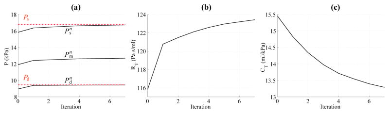
(a) Evolution of systolic ( ), mean ( ) and diastolic ( ) pressure, (b) net peripheral resistance (RT), and (c) total compliance CT with the iteration number (n) for the baseline aorta. The target systolic (Ps) an diastolic (Pd) pressures are shown in red dashed lines.
Other methods have been proposed in the literature to estimate the parameters of the outflow boundary conditions. A root-finding method is described by Spilker and Taylor [53] in the context of 3-D models with compliant arterial walls. Devault et al. proposed a Kalman-filter based methodology in a 1-D model of the circle of Willis [54].
2.6. Error Calculations
The numerical solutions of pressure P and volumetric flow Q were compared between the 1-D and 3-D models using the following relative error metrics [9]:
| (24) |
| (25) |
| (26) |
| (27) |
where Nt is the number of time points where the comparison is made (typically around several thousand points over a single cardiac cycle depending on the time step size), are the pressure and flow results at each time point i from the 1-D simulation at a single spatial location, and are the cross-sectional averaged pressure and flow at each time point i from the 3-D model at a single cross-section perpendicular to the vessel centerline. εP,avg and εQ,avg are the average relative errors for pressure and flow, respectively, over one cardiac cycle, and εP,max and εQ,max are the maximum relative error in pressure and flow. εP,sys and εQ,sys are the errors for systolic pressure and flow, εP,dias and εQ,dias are the errors for diastolic pressure and flow. In order to avoid division by small values of flow, we normalized the flow error metrics by the maximum value of flow over the cardiac cycle, . The error metrics were calculated over a single cardiac cycle once both numerical solutions achieved periodic behavior.
3. RESULTS
We investigated the differences in the numerical prediction of flow and pressure between the 1-D and 3-D formulations (where flow and pressure refer to cross-sectional averages in planes perpendicular to the vessel centerline) in a series of test cases using idealized geometries. The physical dimensions, vessel wall properties, and inflow and outflow boundary conditions were made to be consistent between the 1-D models and their 3-D counterparts. Mesh independence studies were undertaken to ensure that the results in the final meshes were not affected by inadequate mesh resolution.
3.1. Baseline Common Carotid
We considered a straight cylindrical vessel with representative dimensions of the common carotid artery (CCA). The initial total peripheral resistance (RT) and compliance (CT) were calculated from Eqs. (13) and (17), respectively, using a reference value of mean blood pressure (Pm) measured in a 23-year-old human [55, p. 343] and a reference inflow waveform [17]. The final values of RT and CT were then computed as described in Section 2.5, requiring a single iteration to achieve convergence to the target pressures at the outlet. The parameters of the CCA model are given in Table I.
Table I.
Normal hemodynamic properties of the human common carotid artery. The geometry, inflow rate and mechanical properties of the blood were taken from [17], the Young’s modulus E from [65] and the pressures from [55, p. 343]. The parameters of the RCR windkessel model were calculated as described in the text. The resulting wave speed at mean pressure is cm = 6.74 m s−1.
| Property | Value |
|---|---|
| Length, L | 126 mm |
| Radius at diastolic pressure, rd | 3 mm |
| Wall thickness, h | 0.3 mm |
| Young’s modulus, E | 700.0 kPa |
| Mean flow rate, Q̄in | 0.39 l min−1 |
| Systolic pressure, Ps | 16.7 kPa |
| Diastolic pressure, Pd | 10.9 kPa |
| Windkessel resistance, R1 | 2.4875 · 108 Pa s m−3 |
| Windkessel compliance, C | 1.7529 · 1010 m3 Pa−1 |
| Windkessel resistance, R2 | 1.8697 · 109 Pa s m−3 |
The 1-D simulation was run using 6 elements with a quadrature and polynomial order of 10 and a time step of 0.1 ms. The velocity profile order was ζ = 2. The initial area A0 = 0.22 cm2 that yields the reference diastolic area (Ad) at P = Pd was calculated using Eq. (9). The 3-D geometry was constructed with the same dimensions as in the 1-D segment. The velocity on the inlet boundary was prescribed using Eq. (2) with ζ = 2 and with the same time-averaged flow-rate as at the inlet of the 1-D model. The 3-D simulation was run with a mesh containing 792,559 linear tetrahedral elements (145,394 nodes) and a time-step of 0.2 ms.
Fig. 3 shows the numerical predictions of flow rate, pressure, changes in luminal radius, and velocity profiles at several sites in the 1-D and 3-D models. The flow waveforms exhibit the typical attenuation observed in vivo between the inlet and outlet faces. We also include the pressure gradient (given as the difference between inlet and outlet pressures) predicted by the two numerical schemes. The results show excellent agreement between the two models, with average relative errors smaller than 1%. However, even though the flow waveforms in 1-D and 3-D models are virtually identical, differences can be observed in the velocity profiles. These differences result from the linearized kinematics assumption (i.e. fixed computational domain) of the 3-D formulation, in contrast to the 1-D model, which accounts for changes in cross-sectional area. In all the examples considered in this manuscript, the 1-D velocity profiles were plotted in the reference configuration given by the nominal (diastolic) diameter of the vessel to provide a qualitative comparison between the profile shapes.
Figure 3.

Baseline common carotid case. Top: flow rate and pressure with time at the inlet, midpoint and outlet, radius with time at the midpoint, and pressure gradient between inlet and outlet in the 3-D model (solid lines) and 1-D model (dashed lines) with relative error metrics (Section 2.6). Bottom: velocity magnitude in the reference domain of the 3-D model (colormap). Velocity profiles of the 3-D model (solid lines, axial velocity component) and the 1-D model (dashed lines) at three locations and two time points.
3.2. Baseline Aorta
We considered a straight cylinder with diameter representative of the average diameter of the thoracic aorta. Here, the initial peripheral resistance was calculated using systolic and diastolic pressures from [51] and the total compliance CT was calculated from the time constant τ = 1.79 s [51] of the exponential fall-off of pressure during diastole using Eq. (16). The final values of RT and CT were obtained after seven iterations to reach convergence to the target pressures at the outlet. The parameters of the baseline aortic model are given in Table II.
Table II.
Normal hemodynamic properties of the human aorta, from the ascending to the thoracic part. The inflow rate was taken from [50] and the pressures from [51]. The parameters of the RCR windkessel model were calculated as described in the text. The resulting wave speed at mean pressure is cm = 5.17 m s−1.
| Property | Value |
|---|---|
| Length, L | 24.137 cm |
| Radius at diastolic pressure, rd | 1.2 cm |
| Wall thickness, h | 1.2 mm |
| Young’s modulus, E | 400.0 kPa |
| Mean flow rate, Q̄in | 6.170 l min−1 |
| Systolic pressure, Ps | 16.8 kPa |
| Diastolic pressure, Pd | 9.5 kPa |
| Windkessel resistance, R1 | 1.1752 · 107 Pa s m−3 |
| Windkessel compliance, C | 1.0163 · 108 m3 Pa−1 |
| Windkessel resistance, R2 | 1.1167 · 108Pa s m−3 |
For the 1-D model, the simulation was run using 12 elements with a quadrature and polynomial order of 5 and a time step of 0.1 ms. The initial area was calculated using Eq. (9) to be A0 = 3.06 cm2. The polynomial order of the velocity profile was chosen to be ζ = 9 based on [35]. For the 3-D model, the velocity boundary condition at the inlet was prescribed with a profile of order ζ = 9. The 3-D simulation was run using a mesh containing 1,480,048 linear tetrahedral elements (261,912 nodes) and a time step of 0.2 ms.
Fig. 4 shows the numerical predictions of flow rate, pressure, changes in luminal radius, and velocity profiles at several sites in the 1-D and 3-D models. Fig. 4 also contains a plot of the pressure gradient between the inlet and outlet. The overall agreement between the two formulations is still reasonably good, particularly during diastole, with average relative errors smaller than 2%. The largest differences in pressure are seen at the inlet during acceleration, and the largest differences in flow are observed during peak systolic flow at the mid-point and outlet locations. The velocity contours at deceleration (t = 0.33 s) are markedly different: while the 1-D solution preserves the fixed 9th-order velocity profile, the 3-D results show near-wall flow reversal, resulting in a Womersley-like profile. Furthermore, the axisymmetry of the 3-D profile breaks down in the second half of the vessel during peak systole (t = 0.15 s). The pressure gradient plot shows larger absolute differences than in the carotid geometry and a slight phase-lag between the 3-D and 1-D predictions.
Figure 4.

Baseline aorta case. Top: flow rate and pressure with time at the inlet, midpoint and outlet, radius with time at the midpoint, and pressure gradient between inlet and outlet in the 3-D model (solid lines) and 1-D model (dashed lines) with relative error metrics (Section 2.6). Bottom: velocity magnitude in the reference domain of the 3-D model (colormap). Velocity profiles of the 3-D model (solid lines, axial velocity component) and the 1-D model (dashed lines) at three locations and two time points.
3.3. Low Flow, and Larger Diameter Aorta
To study the impact of Reynolds number and flow inertia, we considered two more cases in addition to the baseline straight aorta model. In the first case, the flow prescribed at the inlet was reduced by a factor of 9.54 to match the peak Reynolds number to that of the CCA model (Re = 748). In the second case, the diameter of the cylindrical domain was increased to 1.5 cm from 1.2 cm, while the flow rate and vessel length remained unchanged (Re = 5, 713 at peak systole). Figures 5 and 6 show the flow rate, pressure, change in luminal radius, and pressure gradient at several sites in the 1-D and 3-D models. While reducing the Reynolds number via decreasing the total flow did not decrease the error in the inlet pressures during acceleration (see Fig. 5), increasing the vessel diameter without altering the total flow (Fig. 6) did bring the 3-D and 1-D predictions closer.
Figure 5.

Low-flow aorta case. Top: flow rate and pressure with time at the inlet, midpoint and outlet, radius with time at the midpoint, and the pressure gradient between inlet and outlet in the 3-D model (solid lines) and 1-D model (dashed lines) with relative error metrics (Section 2.6).
Figure 6.

Larger-diameter aorta case. Top: flow rate and pressure with time at the inlet, midpoint and outlet, radius with time at the midpoint, and pressure gradient between inlet and outlet in the 3-D model (solid lines) and 1-D model (dashed lines) with relative error metrics (Section 2.6).
3.4. Tapered Carotid
We considered a linearly tapered cylinder with the same length as the previous CCA geometry. Based on reference values for the degree of tapering of the left CCA in [56], the diameter was set to 8 mm at the inlet and 4 mm at the outlet. Although RT remained unchanged from the non-tapered CCA model, the resistance R1 (see Eq. (15)) was recalculated with the values of cd and Ad at the location of the outlet, giving a value of R1 = 6.8548 · 108 Pa s m−3 and R2 = 1.4330 · 109 Pa sm−3. The remaining parameters were unchanged from those given in Table I.
For the 1-D model, the velocity profile was specified with ζ = 2 and the simulation was carried out using 6 elements with a quadrature and polynomial order of 10 and a time step of 0.1 ms. For the 3-D model, the velocity boundary condition at the inlet was prescribed using a profile of order ζ = 2 and the simulation was run using a mesh containing 840,899 linear tetrahedral elements (153,539 nodes) and a time step of 0.2 ms.
Fig. 7 shows the flow rate, pressure, pressure gradient, velocity profiles and change in luminal radius at several sites in the 1-D and 3-D models. Slightly larger differences in 3-D/1-D predicted pressure are observed at the inlet and in the center of the vessel. Compared to the non-tapered CCA geometry, there is also a significant increase in pressure gradient discrepancy.
Figure 7.

Tapered carotid case. Top: flow rate and pressure with time at the inlet, midpoint and outlet, radius with time at the midpoint, and pressure gradient between inlet and outlet in the 3-D model (solid lines) and 1-D model (dashed lines) with relative error metrics (Section 2.6). Bottom: velocity magnitude in the reference domain of the 3-D model (colormap). Velocity profiles of the 3-D model (solid lines, axial velocity component) and the 1-D model (dashed lines) at three locations and two time points.
3.5. Tapered Aorta
We considered a linearly tapered cylinder with length identical to that of the baseline non-tapered aorta model. Based on typical reported aortic dimensions [56], the diameter was set to 3 cm at the inlet and 2 cm at the outlet. RT remained unchanged from the baseline non-tapered aorta model, but the resistance R1 was recalculated with the values of cd and Ad at the location of the outlet. We obtained R1 = 1.8503 · 107 Pa s m−3 and R2 = 1.0492 · 108 Pa s m−3. The remaining parameters were unchanged from those in Table II.
For the 1-D model, the polynomial order of the velocity profile was chosen to be ζ = 9 and the 1-D simulation was run using 12 elements with a quadrature and polynomial order of 5 and a time step of 0.1 ms. For the 3-D model, the velocity boundary condition at the inlet boundary was prescribed using a profile of order ζ = 9 and the simulation was run using a mesh containing 1,663,772 linear tetrahedral elements (293,667 nodes) and a time step of 0.2 ms.
Fig. 8 shows the flow rate, pressure, changes in luminal radius, velocity profile, and pressure gradient at several sites in the 1-D and 3-D models. Results show larger differences in pressure and flow waveforms at the midpoint and inlet locations, respectively, compared to those found in the tapered carotid case. The differences between the velocity contours are also more noticeable, with the 3-D profile displaying near-wall flow-reversal patterns.
Figure 8.

Tapered aorta case. Top: flow rate and pressure with time at the inlet, midpoint and outlet, radius with time at the midpoint, and pressure gradient between inlet and outlet in the 3-D model (solid lines) and 1-D model (dashed lines) with relative error metrics (Section 2.6). Bottom: velocity magnitude in the reference domain of the 3-D model (colormap). Velocity profiles of the 3-D model (solid lines, axial velocity component) and the 1-D model (dashed lines) at three locations and two time points.
3.6. Aorta with Curvatures
We considered two additional aortic models using the same inflow and outflow boundary conditions as the baseline aorta model with the purpose of studying the impact of vessel curvature on cross-sectional average pressure and velocity. In the first case, curvature was introduced in a single plane (sagittal) to represent an idealized aortic arch. In the second case, curvatures were introduced in three planes (sagittal, coronal, and transverse) as described by Yearwood and Chandran [57]. Lengths and diameters were kept unchanged relative to the baseline aorta case. Since the 1-D model is independent of curvature, the 1-D solution is identical to that obtained in Section 3.2. The boundary conditions and material parameters were identical to those in the baseline aorta model (see Table II).
Due to the centripetal loading experienced by the vessel wall in the curved portion of the 3-D geometry, a small value for the external damping coefficient (cs = 300 Pa s m−1) was chosen to reduce nonphysiological oscillatory modes. The external damping smooths the pressure and flow waveforms predominantly where high frequencies are dominant, with distal waveforms being smoother than proximal ones. These results are in agreement with the linear analysis of wall viscoelasticity described in [50]. The simulation of the 3-D model containing the single plane of curvature was run using a mesh containing 1,691,525 linear tetrahedral elements (297,472 nodes) and a time step of 0.2 ms. The model containing three planes of curvature was simulated with a mesh containing 1,688,467 linear tetrahedral elements (297,083 nodes) and a time step of 0.2 ms.
Figures 9 and 10 show the flow rate, pressure, changes in luminal radius, and pressure gradient for the single-curvature and three-curvature cases, respectively, and compares them with the corresponding 1-D predictions, which are the same as those shown in Fig. 4. In-plane and out-of-plane velocity profiles at three cross sections in the 3-D models illustrate the skewing of the velocity profile toward the outer wall during systole and the presence of backflow along the inner wall during diastole. Nevertheless, the relative errors in flow, pressure, and pressure gradient are similar to those observed in the baseline aorta case.
Figure 9.

Single-curvature aorta case. Top: flow rate and pressure with time at the inlet, midpoint and outlet, radius with time at the midpoint, and pressure gradient between inlet and outlet in the 3-D model (solid lines) and 1-D model (dashed lines) with relative error metrics (Section 2.6). Bottom: in-plane (colormap and arrows, left) velocity and out-of-plane (colormap, right) components of the velocity field in the 3-D model at three cross-sections. Velocities are given in cm/s. The outer and inner curvatures are labeled as “O” and “I”, respectively.
Figure 10.

Multiple-curvature aorta case. Top: flow rate and pressure with time at the inlet, midpoint and outlet, radius with time at the midpoint, and the pressure gradient between inlet and outlet in the 3-D model (solid lines) and 1-D model (dashed lines) with relative error metrics (Section 2.6). Bottom: in-plane (colormap and arrows, left) velocity and out-of-plane (colormap, right) components of the velocity field in the 3-D model at three cross-sections. Velocities are given in cm/s. The outer and inner curvatures are labeled as “O” and “I”, respectively.
3.7. Aortic Bifurcation
Here, we considered an idealized model of the aortic bifurcation, containing a single parent segment, representing the abdominal aorta, and two branch segments representing the iliac arteries. The lengths and diameters are listed in Table III. The initial net peripheral resistance and total compliance were calculated from Equations (13) and (17) using the systolic and diastolic pressures from [51]. The final values of RT and CT were obtained after three iterations to reach convergence to the target pressures at the inlet. The peripheral resistance R1 + R2 at the outlet of the iliac arteries was calculated assuming equal flow distribution.
Table III.
Normal hemodynamic properties of the human aortic bifurcation. The dimensions are based on data given in [3]. The flow rate is taken from [66] and the pressures from [51]. The parameters of the two RCR models were calculated as described in the text. The resulting wave speed at mean pressure is cm = 6.26 m s−1 in the abdominal aorta and cm = 7.4 m s−1 in both iliac arteries.
| Property | Aorta | Iliac |
|---|---|---|
| Length, L | 8.6 cm | 8.5 cm |
| Radius at diastolic pressure, rd | 0.86 cm | 0.60 cm |
| Wall thickness, h | 1.032 mm | 0.72 mm |
| Young’s modulus, E | 500.0 kPa | 700.0 kPa |
| Mean flow rate, Q̄in | 0.4791 l min−1 | |
| Systolic pressure, Ps | 16.8 kPa | |
| Diastolic pressure, Pd | 9.5 kPa | |
| Windkessel resistance, R1 | – | 6.8123 · 107 Pa s m−3 |
| Windkessel compliance, C | – | 3.6664 · 1010 m3 Pa−1 |
| Windkessel resistance, R2 | – | 3.1013 · 109Pa s m−3 |
For the 1-D model, the simulation was run using 12 elements with a quadrature and polynomial order of 5 and a time step of 0.1 ms. The initial area was calculated using Eq. (9) to be A0 = 1.8062 cm2 in the abdominal aorta and A0 = 0.9479 cm2 in the iliac branches. The velocity profile was chosen to have a polynomial order ζ = 9. For the 3-D model, the geometry was constructed from three cylinders with the same diameters and lengths as in the 1-D network. The angle between the two iliac branches was set to 47.9 degrees [58]. The velocity boundary condition at the inlet was prescribed with a profile of order ζ = 9. The simulation was run using a mesh containing 1,799,117 linear tetrahedral elements (321,651 nodes) and a time step of 0.2 ms.
Fig. 11 shows the flow rate, pressure, velocity and changes in luminal radius at several sites in the 1-D and 3-D models. The results show excellent agreement between the two models (average relative errors smaller than 2%), with similar relative errors to the baseline common carotid artery case.
Figure 11.

Aortic bifurcation case. Top: flow rate, pressure, change in radius with time at several locations and pressure gradient between inlet and outlet in the 3-D model (solid lines) and 1-D model (dashed lines) with relative error metrics (Section 2.6). Bottom: velocity magnitude in the reference domain of the 3-D model (colormap). Velocity profiles of the 3-D model (solid lines, axial velocity component) and the 1-D model (dashed lines) at three locations and two time points.
3.8. Full Aorta
We considered an idealized geometry representing the aorta and the first generation of main branches from just above the sinuses to the aortic bifurcation, neglecting the coronary and intercostal vessels. The curvature and angulation from the sagittal plane in the aortic arch were based on published measurements from human cadavers [57, 59]. The dimensions and spacing between branch vessels were based on those reported in [3]. The parameters are summarized in Table IV and the geometry is illustrated in Fig. 12. The spatially-varying elastic moduli (E) were calculated from the pulse wave velocity, c, given by the empirical relationship [56] c = a2/(2rd)b2, where c is given in m/s, rd is the radius at diastolic pressure expressed in mm, a2 = 13.3 and b2 = 0.3. For each vessel segment, once c was determined, E was calculated using Eq. (8) with A = Ad. The spatially-varying wall thickness (h) was chosen to be 10% of rd [55] at the inlet of each segment.
Table IV.
Parameters of the full-aorta model. rin → rout: diastolic cross-sectional radii at the inlet and outlet of the arterial segment. cin → cout: wave speed at diastolic pressure at the inlet and outlet of the arterial segment.
| Arterial segment | Length (cm) | rin → rout (mm) | cin → cout (m/s) | R1 (107 Pa s m−3) | R2 (108 Pa m−3) | C(10−10 m3 Pa−1) |
|---|---|---|---|---|---|---|
| 1. Ao I | 7.0357 | 15.2 → 13.9 | 4.77 → 4.91 | - | - | - |
| 2. Ao II | 0.8 | 13.9 → 13.7 | 4.91 → 4.93 | - | - | - |
| 3. Ao III | 0.9 | 13.7 → 13.5 | 4.93 → 4.94 | - | - | - |
| 4. Ao IV | 6.4737 | 13.5 → 12.3 | 4.94 → 5.09 | - | - | - |
| 5. Ao V | 15.2 | 12.3 → 9.9 | 5.09 → 5.43 | - | - | - |
| 6. Ao VI | 1.8 | 9.9 → 9.7 | 5.43 → 5.46 | - | - | - |
| 7. Ao VII | 0.7 | 9.7 → 9.62 | 5.46 → 5.48 | - | - | - |
| 8. Ao VIII | 0.7 | 9.62 → 9.55 | 5.48 → 5.49 | - | - | - |
| 9. Ao IX | 4.3 | 9.55 → 9.07 | 5.49 → 5.57 | - | - | - |
| 10. Ao X | 4.3 | 9.07 → 8.6 | 5.57 → 5.66 | - | - | - |
| 11. Brachiocephalic | 3.4 | 6.35 → 6.35 | 6.20 → 6.20 | 5.1918 | 10.6080 | 8.6974 |
| 12. L com. carotid | 3.4 | 3.6 → 3.6 | 7.36 → 7.36 | 19.1515 | 52.2129 | 1.7670 |
| 13. L subclavian | 3.4 | 4.8 → 4.8 | 6.75 → 6.75 | 9.8820 | 13.0183 | 7.0871 |
| 14. Celiac | 3.2 | 4.45 → 4.45 | 6.90 → 6.90 | 11.7617 | 7.5726 | 12.1836 |
| 15. Sup. mesenteric | 6 | 3.75 → 3.75 | 7.27 → 7.27 | 17.4352 | 5.5097 | 16.7453 |
| 16. R renal | 3.2 | 2.8 → 2.8 | 7.93 → 7.93 | 34.1378 | 5.3949 | 17.1017 |
| 17. L renal | 3.2 | 2.8 → 2.8 | 7.93 → 7.93 | 34.1378 | 5.3949 | 17.1017 |
| 18. Inf. mesenteric | 5 | 2.0 → 2.0 | 8.77 → 8.77 | 74.0167 | 46.2252 | 1.9959 |
| 19. R com. iliac | 8.5 | 6.0 → 6.0 | 6.31 → 6.31 | 5.9149 | 10.1737 | 9.0686 |
| 20. L com. iliac | 8.5 | 6.0 → 6.0 | 6.31 → 6.31 | 5.9149 | 10.1737 | 9.0686 |
Figure 12.

Idealized full aorta geometry and vessel wall material properties. (a): coronal (left) and sagittal (right) views with lengths and diameters. (b): close-up view of the arch and branches with lengths and diameters and the primary radius of curvature. (c): close-up view of the arch showing the degree of curvature in the ascending arch (left) and transverse view of the arch (right), showing the degree of transverse curvature and the degree of angulation from the sagittal plane. (d): the spatial distributions of wall thickness (h) and elastic modulus (E).
The total peripheral resistance RT = 1.1583 · 108 Pa s m−3 was obtained from Eq. (13) with Q̄in = 6.17 l min−1 Ps = 16.8 kPa and Pd = 9.5 kPa. At the outlet of each terminal branch, the resistance R1 + R2 was calculated to yield the flow distribution given in [2] (see Table V). Each resistance R1 follows from Eq. (15) with cd and rd calculated at the outlet of the terminal branch. The total compliance CT was calculated from the time constant τ = 1.79 s [51] of the exponential fall-off of pressure during diastole using Eq. (16); CT = τ/RT = 1.5453 · 10−8 m3 Pa−1. The compliance C of each terminal RCR model was then calculated as described in Section 2.5. The final values of RT and CT were obtained after eight iterations to reach convergence to the target pressures at the outlet of the abdominal aorta.
Table V.
Distribution of the cardiac output among each terminal vessel in the full aorta model.
| Terminal vessel | % cardiac output |
|---|---|
| 11. Brachiocephalic | 10.41 |
| 12. L com. carotid | 2.14 |
| 13. L subclavian | 8.27 |
| 14. Celiac | 13.24 |
| 15. Sup. mesenteric | 15.97 |
| 16. R renal | 13.15 |
| 17. L renal | 13.15 |
| 18. Inf. mesenteric | 2.16 |
| 19. R com. iliac | 10.76 |
| 20. L com. iliac | 10.76 |
For the 1-D model, the simulation was run using 46 elements with a quadrature and polynomial order of 5 in each vessel and a time step of 0.05 ms. The initial areas A0 that yield the diastolic areas Ad at P = Pd were calculated using Eq. (9) (A0 = 4.7203 cm2 at the aortic root). The velocity profile was chosen with polynomial order ζ = 9. For the 3-D model, the external damping coefficient was assigned a small value (cs = 300 Pa s m−1) to reduce non-physiological oscillations. The simulation was run using a mesh containing 2,554,521 linear tetrahedral elements (475,000 nodes) and a time-step of 0.2 ms. The velocity boundary condition at the inlet was prescribed with a profile of order ζ = 9.
Fig. 13 shows flow rate and pressure at a number of representative locations in the 1-D and 3-D models. The differences in the pressure and flow predictions occur predominantly in peak systole, and these discrepancies are greater in distal sites than in the proximal aortic arch branches. Additionally, the results from the 3-D model exhibit fewer high-frequency features in the flow and pressure waveforms than in the 1-D model as a consequence of external damping.
Figure 13.

Full aorta case. Flow rate (left) and pressure (right) with time at 8 outlets in the 3-D model (solid lines) and 1-D model (dashed lines) with relative error metrics (Section 2.6).
4. DISCUSSION
4.1. Carotid vs. Aortic Geometry: Combined Impact of Reynolds Number, Wall Strain and Velocity Profile
In the baseline carotid case, the assumptions of the 1-D formulation, i.e. predominantly unidirectional flow, hold well. The relative errors in flow and pressure were small between the 1-D and 3-D carotid models, with εP,avg and εQ,avg generally less than 0.3%, as shown in Fig. 3. In the baseline aorta case, however, the differences between the 1-D and 3-D models were greater (Fig. 4), particularly at the inlet, where the 3-D model shows a more pronounced systolic “shoulder” (at t ≈ 0.1 s) in the pressure waveform compared to the 1-D model. Furthermore, the pressure gradient between the inlet and outlet is greater in the 3-D model during peak systole and also exhibits a phase-lag between the 1-D and 3-D models, i.e., the time at which the pressure gradient from the 3-D model reverses direction during systole is delayed compared to the 1-D model.
Inertial forces play a larger role in the aorta model compared to the carotid model, with the peak Reynolds number in the aorta model being nearly an order of magnitude greater than in the carotid model (Re = 7, 140 vs Re = 748). To investigate the impact of the Reynolds number in the pressure waveforms, we scaled down, by a factor of 9.54, the aorta model inflow to match the peak Reynolds number of the baseline carotid model. We observed that the average relative error in the pressure waveforms at the midpoint and outlet locations decreased, but the relative errors at the shoulder of the inlet pressure waveform and the phase lag in the pressure gradient were not reduced (Fig. 5).
To investigate the origin of these discrepancies further, we must reflect on the different treatments that our specific 1-D and 3-D implementations make regarding geometric nonlinearities. While both formulations consider equivalent linear material laws, the 3-D formulation assumes a linearized kinematics behavior for the vessel wall (i.e., a fixed computational grid is maintained throughout the simulation), whereas the 1-D formulation accounts for changes in cross-sectional area (see Eq. (7)). Therefore, the fixed-grid assumption of the 3-D formulation introduces errors in the velocity profile that are proportional in magnitude to the vessel wall strain. The aorta experiences both greater flow velocities and larger wall strains (ε = Δrmax/rd) compared to the carotid setting (i.e. εaortic = 12.5% versus εcarotid = 6%). These two phenomena are responsible for the larger discrepancies between the 1-D and 3-D results during systole in the baseline aorta compared to the carotid example. This idea is supported by the larger diameter aorta model. Despite being a more compliant model than the baseline aorta (due to a larger cross-sectional area), it experiences smaller wall strains. The centerline velocities are also reduced compared to the baseline aorta model. We therefore have a situation where both the Reynolds number and the wall strains are reduced. This ultimately results in a smaller relative error in the shoulder of the inlet pressure waveform (Fig. 6) compared to the baseline aorta model (Fig. 4).
4.2. Impact of Tapering
The presence of tapering introduces errors between the 1-D and 3-D model in the systolic pressure (but not during the diastolic decay) in both carotid and aortic models (Figs. 7 and 8). The 3-D model more accurately captures the spatial changes in the velocity profile, and therefore, the viscous friction losses in the tapered tube. With tapering we observed greater errors between the 1-D and 3-D model in the pressure gradient between the inlet and outlet, as the 3-D model predicts that a greater pressure gradient is needed to drive flow during peak systole. In the tapered aorta case, inertial and frictional effects are naturally better captured in the 3-D model, resulting in greater errors in the pressure waveform than in the tapered carotid case.
4.3. Impact of Curvature
The velocity field in the curved 3-D domain is complex and not axisymmetric (Figs. 9 and 10). During systole, the region of higher velocity is located near the outer wall of the arch, and during deceleration, significant backflow occurs near the inner wall. As such, the 3-D model is inherently more accurate in capturing the inertial and frictional forces in the curved domain, which leads to differences in the integrated flow and pressure quantities compared to the 1-D model. Hence, we observed that the addition of a single plane of curvature slightly increased the relative errors in the pressure and flow waveforms (Fig. 9) compared to the uncurved baseline aorta case. In particular, the error in the systolic shoulder of the inlet pressure waveform was notably increased (compare Figs. 4 and 9).
External damping was necessary in the 3-D model to produce flow and pressure waves without spurious oscillations. This damping was not included in the 1-D formulation and contributes to some of the discrepancies observed. The added dissipation attenuated the high-frequency features of the flow and pressure waveforms in the 3-D model, whereas these features are more prominent in the 1-D model; i.e. the dicrotic notch and the early-diastolic flow reversal phase. We further observed that the addition of the second and third planes of curvature to the 3-D model did not further introduce significant differences between the 3-D and 1-D predictions (Fig. 10) compared to the single curvature case (Fig. 9). In Section 4.5 we investigate the relationship between external damping and curvature in the 3-D setting.
4.4. Bifurcation
The 1-D and 3-D model are in good agreement in the aortic bifurcation case. We observed small relative errors (average relative errors smaller than 2%) between the 1-D and 3-D models (Fig. 11), which was expected considering the lower flow rate in comparison to the aorta case. Furthermore, changing the bifurcation angle from 47.9 degrees to 27.5 degrees resulted in a negligible change in the relative errors. A similar good agreement was obtained with a geometric model of the abdominal aorta featuring two 90 degree branches representing the renal arteries. These results suggest that the effect of energy losses at the aortic bifurcation on the pressure waveforms is minor, as was previously observed using in-vitro data [22].
4.5. Full Aorta Comparison
The full aorta model is essentially a combination of all the previously considered geometric features, including tapering, curvature, branching, and a variety of vessel diameters. As such, we expected to observe larger differences in the prediction of flow and pressure waveforms between the two theories. In general, the largest differences occur in systole, whereas the diastolic predictions are much closer. We can explain the closer agreement between models during diastole using a 0-D Windkessel model for pressure. Starting with the 1-D formulation, a space-independent Windkessel pressure, pw(t), can be derived by neglecting nonlinearities, flow inertia and viscous dissipation, and assuming that wall compliance and fluid peripheral resistance are the dominant effects [52]. Under these premises, pw(t) is given by
| (28) |
where Qin(t) is the flow waveform at the inlet of the ascending aorta, pw(T0) is the pressure pw at t = T0, T0 is the time corresponding to the beginning of systole (T0 = 0 in Fig. 14 ), M − 1 < N is the number of terminal branches, and is the outflow in the terminal Segment j. The net peripheral resistance (RT) is given by Eq. (14), and the total arterial compliance (CT) is given by Eq. (18). The parameters of the RCR Windkessel models are R1, C, R2 and Pout (Fig. 1 ). The validity of Eq. (28) is also supported by in-vivo studies, which show that the aortic pressure waveform is approximately uniform in space during approximately the last two thirds of diastole [60, 61].
Figure 14.

Left: Analytical prediction of pressure (dotted lines) shows good agreement with 1-D and 3-D models during diastole. Right: Pressure and flow rate at the midpoint of the abdominal aorta for the curved 3-D aorta tree model with external damping (red), the straight 3-D aorta model with external damping (dashed blue), the straight 3-D aorta model without external damping (dashed green), and the 1-D model (dashed black). The level of external damping cs = 300 Pa s m−1 and is identical for all the 3-D models.
The waveforms for the straight 3-D model with and without damping are essentially identical.
Figure 14 (left) illustrates that the agreement between 3-D, 1-D and analytical pressures improves as diatole progresses, indicating that the physics of flow are fundamentally linear and inertia-free during this phase of the cardiac cycle. Conversely, systolic flow is fundamentally non-linear and advection/inertia dominated, and therefore larger differences between the two methods were observed.
The discrepancies observed in systole are partially due to the different treatment of the arterial wall mechanics in the two formulations: while both theories consider equivalent purely elastic material laws, the 3-D case requires a viscous dissipation term provided by the external tissue support model. Without this dissipation, the 3-D flow and pressure waveforms contain spurious, large amplitude high-frequency oscillations resulting from unconstrained rigid-body motion modes that are generated in non-axisymmetric flows. This viscous damping, while necessary in the 3-D setting, attenuated the sharper features of the flow and pressure waveforms, most noticeably in the dicrotic notch and early-diastole flow reversal phases, compared to the predictions seen in the 1-D setting (Fig. 13).
It is worth noting that external tissue support can also be included in 1-D modeling, as recently demonstrated by [33]. That work focuses on the importance of including external tissue support in the 1-D formulation to reduce reflections at the 1-D/3-D interfaces. Furthermore, while the external tissue support will never be engaged in a 1-D setting to limit spurious wall motion as in the 3-D model, its presence will affect the deformation of the arterial wall due to the additional stiffness. Figure 14 (right) illustrates the impact of external tissue damping by introducing a new model consisting of a modified “straightened” full aorta geometry. We compared infrarenal flow and pressure waveforms in four different cases: 1) 3-D formulation in original full aorta geometry considering tissue damping; 2) 3-D fomulation in straightened full aorta geometry considering tissue damping; 3) 3-D formulation in straightened full aorta geometry without tissue damping; and 4) 1-D formulation. The results in the straightened 3-D aorta models (dashed blue and green lines) demonstrated sharper features than those observed in the 3-D curved aorta model (solid red lines) and, notwithstanding the larger pulse pressures in the 3-D model, resembled more closely the results from the 1-D model (dashed black lines). Furthermore, the exclusion of external tissue damping (green dashed lines) resulted in almost no difference in the pressure and flow waveforms in the straightened model. This behavior suggests that eliminating the aortic curvature reduced the rigid-body modes in the thoracic region and, even though the external viscous damping is still present, it is engaged to a lesser degree than in the original curved aorta model.
4.6. Limitations
It is important to note that the comparisons presented in this paper were between two particular implementations of 1-D and 3-D theories with equivalent boundary conditions and material laws. However, a one-to-one comparison of hemodynamics between the two theories is not always possible. A few examples of fundamental modeling differences that are not easy to overcome are: the inability to account for secondary flows and the assumption of a fixed velocity profile in the 1-D formulation; the linearized kinematics approach and the need for outflow boundary condition stabilization and external tissue support in the 3-D formulations.
To facilitate an improved comparison, the 1-D formulation could incorporate space- and time-varying velocity profiles [7, 56, 62, 63, 64]. Furthermore, external damping [9] and wall inertia [5] could be included in the 1-D model as well. On the other hand, the 3-D formulation would need to incorporate moving domains/meshes [11, 16] to enable a more consistent description of cross-sectional area changes between the two methods.
4.7. Implications of Fundamental Modeling Differences between 3-D and 1-D Theories
An inconsistency between our specific 1-D and 3-D implementations was introduced by assigning zero velocity boundary conditions at the inlet and outlet rings in the 3-D model, effectively clamping the vessels at those locations. Consequently, the conduit compliance (Cc) of the vessels in the 3-D models is slightly reduced relative to the 1-D models; this becomes more significant as the length of the vessel domain decreases. The clamping has a negligible local effect on pressure and flow in the 3-D domain, even though the wall displacements near the inlets and outlets are reduced. A better treatment of the arterial wall boundary conditions in the 3-D formulation can be done using external tissue support formulations [39] and time-resolved medical-image data to inform both the radial and longitudinal components of the vessel wall motion. Lastly, an important inconsistency between our two modeling approaches is introduced by the need for external damping in the 3-D model in complex and curved geometries, such as the curved aorta and full aorta.
5. CONCLUSIONS
In this article, we have compared 1-D and 3-D hemodynamics in a series of idealized compliant arterial models of the carotid artery, thoracic aorta, aortic bifurcation and full aorta. The 1-D and 3-D formulations share common inflow and outflow boundary conditions and have equivalent material laws. We also presented an iterative algorithm to determine the parameters of each outflow boundary condition module to achieve desired systolic and diastolic pressures at a particular vessel. We have demonstrated good agreement between 1-D and 3-D predictions, especially during diastole. The larger differences in systole can be explained by the following: 1) the inability to account for secondary flow features, vessel curvature and a prescribed velocity profile shape in the 1-D model; and 2) the linearized treatment of the kinematics of the vessel wall and the external tissue support (which introduces viscous damping) in the 3-D model.
Our 1-D/3-D framework demonstrates the use of a 1-D model to determine boundary condition and material parameters that are subsequently fed to a corresponding 3-D model. Indeed, the relatively good agreement between the numerical predictions in the full aorta setting suggests that the 1-D model is a reasonable representation of the 3-D system in terms of the global behavior of the spatially-averaged pressure and flow waveforms. It follows that the 1-D model can be used to perform tasks such as 1) estimation of the parameters of outflow boundary conditions to reproduce clinical measurements and 2) sensitivity studies under different hemodynamic conditions to gain an understanding of the behavior of the arterial system. This overlapping 1-D/3-D approach will accelerate the selection of model parameters for 3-D subject-specific models.
Acknowledgments
N. X. and C. A. F. gratefully acknowledge support from the United States National Institutes of Health (NIH) grant R01 HL-105297, the European Research Council under the European Union’s Seventh Framework Programme (FP/2007-2013) / ERC Grant Agreement n. 307532, and the United Kingdom Department of Health via the National Institute for Health Research (NIHR) comprehensive Biomedical Research Centre award to Guy’s & St Thomas’ NHS Foundation Trust in partnership with King’s College London and King’s College Hospital NHS Foundation Trust. J.A. gratefully acknowledges the support of a British Heart Foundation Intermediate Basic Science Research Fellowship (FS/09/030/27812) and the Centre of Excellence in Medical Engineering funded by the Wellcome Trust and EPSRC under grant number WT 088641/Z/09/Z. The 3-D simulations were supported in part by a NSF Extreme Science and Engineering Digital Environment (XSEDE) startup allocation. Lastly, the authors acknowledge Emeritus Professor Kim H. Parker for his critical review of the manuscript, Desmond Dillon-Murphy for his assistance with the generation of the CAD geometry of the full aorta and Simmetrix, Inc. (http://www.simmetrix.com/) for their MeshSim mesh generation library.
References
- 1.Hughes T, Lubliner J. On the one-dimensional theory of blood flow in the larger vessels. Math Biosciences. 1973;18:161–170. [Google Scholar]
- 2.Stergiopulos N, Young DF, Rogge TR. Computer simulation of arterial flow with applications to arterial and aortic stenoses. Journal of Biomechanics. 1992 Dec;25(12):1477–88. doi: 10.1016/0021-9290(92)90060-e. URL http://www.ncbi.nlm.nih.gov/pubmed/1491023. [DOI] [PubMed] [Google Scholar]
- 3.Reymond P, Bohraus Y, Perren F, Lazeyras F, Stergiopulos N. Validation of a Patient-Specific 1-D Model of the Systemic Arterial Tree. American Journal of Physiology Heart and Circulatory Physiology. 2011 May;301(May):H1173–H1182. doi: 10.1152/ajpheart.00821.2010. URL http://www.ncbi.nlm.nih.gov/pubmed/21622820. [DOI] [PubMed] [Google Scholar]
- 4.Olufsen M, Peskin C, Kim W, Pedersen E, Nadim A, Larsen J. Numerical simulation and experimental validation of blood flow in arteries with structured-tree outflow conditions. Annals Biomed Eng. 2000;28:1281–1299. doi: 10.1114/1.1326031. [DOI] [PubMed] [Google Scholar]
- 5.Formaggia L, Lamponi D, Quarteroni A. One-dimensional models for blood flow in arteries. J Eng Math. 2003;47:251–276. [Google Scholar]
- 6.Sherwin SJ, Franke V, Peiro J, Parker KH. One-dimensional modelling of a vascular network in space-time variables. Journal of Engineering Mathematics. 2003 Dec;47(3):217–250. doi: 10.1023/B:ENGI.0000007979.32871.e2. URL http://www.springerlink.com/openurl.asp?id=doi:10.1023/B:ENGI.0000007979.32871.e2 http://www.springerlink.com/index/r33k14217n7130gt.pdf. [DOI] [Google Scholar]
- 7.Bessems D, Rutten M, van de Vosse F. A wave propagation model of blood flow in large vessels using an approximate velocity profile function. J Fluid Mech. 2007;580:145–168. [Google Scholar]
- 8.Mynard J, Nithiarasu P. A 1D arterial blood flow model incorporating ventricular pressure, aortic valve and regional coronary flow using the locally conservative Galerkin (LCG) method. Commun Numer Meth Eng. 2008;24:367–417. [Google Scholar]
- 9.Alastruey J, Khir AW, Matthys KS, Segers P, Sherwin SJ, Verdonck PR, Parker KH, Peiró J. Pulse wave propagation in a model human arterial network: Assessment of 1-D visco-elastic simulations against in vitro measurements. Journal of Biomechanics. 2011 Aug;44(12):2250–8. doi: 10.1016/j.jbiomech.2011.05.041. URL http://www.pubmedcentral.nih.gov/articlerender.fcgi?artid=3278302&tool=pmcentrez&rendertype=abstract. [DOI] [PMC free article] [PubMed] [Google Scholar]
- 10.Müller L, Toro E. Well balanced high order solver for blood flow in networks of vessels with variable properties. International Journal for Numerical. 2013 doi: 10.1002/cnm.2580. http://onlinelibrary.wiley.com/doi/10.1002/cnm.2580/full. [DOI] [PubMed]
- 11.Perktold K, Rappitsch G. Computer simulation of local blood flow and vessel mechanics in a compliant carotid artery bifurcation model. Journal of Biomechanics. 1995 Jul;28(7):845–56. doi: 10.1016/0021-9290(95)95273-8. URL http://www.ncbi.nlm.nih.gov/pubmed/7657682. [DOI] [PubMed] [Google Scholar]
- 12.Taylor CA, Hughes TJR, Zarins CK. Finite element modeling of blood flow in arteries. Computer Methods in Applied Mechanics and Engineering. 1998;7825(97) http://www.sciencedirect.com/science/article/pii/S004578259880008X. [Google Scholar]
- 13.Quarteroni A, Tuveri M, Veneziani A. Computational vascular fluid dynamics: problems, models and methods. Computing and Visualization in Science. 2000 Mar;2:163–97. [Google Scholar]
- 14.Steinman D, Milner J, Norley C, Lownie S, Holdsworth D. Image-based computational simulation of flow dynamics in a giant intracranial aneurysm. American Journal of Neuroradiology. 2003 Apr;24(4):559–566. [PMC free article] [PubMed] [Google Scholar]; 4th World Congress of Biomechanics; Calgary, Canada. Aug, 2002. [Google Scholar]
- 15.Cebral J, Castro M, Burgess J, Pergolizzi R, Sheridan M, Putman C. Characterization of cerebral aneurysms for assessing risk of rupture by using patient-specific computational hemodynamics models. American Journal of Neuroradiology. 2005 Nov-Dec;26(10):2550–2559. [PMC free article] [PubMed] [Google Scholar]
- 16.Gerbeau JF, Vidrascu M, Frey P. Fluid-structure interaction in blood flows on geometries based on medical imaging. Computers & Structures. 2005 Jan;83(2–3):155–165. doi: 10.1016/j.compstruc.2004.03.083. URL http://linkinghub.elsevier.com/retrieve/pii/S0045794904003001. [DOI] [Google Scholar]
- 17.Figueroa CA, Vignon-Clementel IE, Jansen KE, Hughes TJR, Taylor CA. A coupled momentum method for modeling blood flow in three-dimensional deformable arteries. Computer Methods in Applied Mechanics and Engineering. 2006 Aug;195(41–43):5685–5706. doi: 10.1016/j.cma.2005.11.011. URL http://linkinghub.elsevier.com/retrieve/pii/S004578250500513X. [DOI] [Google Scholar]
- 18.van de Vosse F, Stergiopulos N. Pulse wave propagation in the arterial tree. Annu Rev Fluid Mech. 2011;43:467–499. [Google Scholar]
- 19.Alastruey J, Parker K, Sherwin S. Arterial pulse wave haemodynamics. Proc. BHR Group’s 11th International Conference on Pressure Surges; Lisbon, Portugal. 24th – 26th October; 2012. pp. 401–442. [Google Scholar]
- 20.Parker K. An introduction to wave intensity analysis. Med Bio Eng Comput. 2009;47:175–188. doi: 10.1007/s11517-009-0439-y. [DOI] [PubMed] [Google Scholar]
- 21.Steele B, Wan J, Ku J, Hughes T, Taylor C. In vivo validation of a one-dimensional finite-element method for predicting blood flow in cardiovascular bypass grafts. Ieee Transactions On Biomedical Engineering. 2003 Jun;50(6):649–656. doi: 10.1109/TBME.2003.812201. [DOI] [PubMed] [Google Scholar]
- 22.Matthys KS, Alastruey J, Peiro J, Khir AW, Segers P, Verdonck PR, Parker KH, Sherwin SJ. Pulse wave propagation in a model human arterial network: Assessment of 1-D numerical simulations against in vitro measurements. Journal Of Biomechanics. 2007;40(15):3476–3486. doi: 10.1016/j.jbiomech.2007.05.027. [DOI] [PubMed] [Google Scholar]
- 23.Humphrey J, Strumpf R, Yin F. Determination of a constitutive relation for passive myocardium. 2. Parameter-estimation. Journal of Biomechanical Engineering - Transactions of the ASME. 1990 Aug;112(3):340–346. doi: 10.1115/1.2891194. [DOI] [PubMed] [Google Scholar]
- 24.Xiong G, Figueroa CA, Xiao N, Taylor CA. Simulation of blood flow in deformable vessels using subject-specific geometry and spatially varying wall properties. International Journal for Numerical Methods in Biomedical Engineering. 2011 Jul;27(7):1000–1016. doi: 10.1002/cnm.1404. [DOI] [PMC free article] [PubMed] [Google Scholar]
- 25.Prasad A, Xiao N, Gong XY, Zarins C, Figueroa CA. A computational framework for investigating the positional stability of aortic endografts. Biomechanics and Modeling in Mechanogiology. doi: 10.1007/s10237-012-0450-3. [DOI] [PMC free article] [PubMed] [Google Scholar]
- 26.Taylor CA, Figueroa CA. Patient-specific modeling of cardiovascular mechanics. Annual Review of Biomedical Engineering. 2009 Jan;11(April):109–34. doi: 10.1146/annurev.bioeng.10.061807.160521. URL http://www.ncbi.nlm.nih.gov/pubmed/19400706. [DOI] [PMC free article] [PubMed] [Google Scholar]
- 27.Moore S, Moorhead K, Chase J, David T, Fink J. One-dimensional and three-dimensional models of cerebrovascular flow. Journal Of Biomechanical Engineering-transactions Of The Asme. 2005 Jun;127(3):440–449. doi: 10.1115/1.1894350. [DOI] [PubMed] [Google Scholar]
- 28.Grinberg L, Cheever E, Anor T, Madsen JR, Karniadakis GE. Modeling blood flow circulation in intracranial arterial networks: a comparative 3D/1D Simulation Study. Annals Of Biomedical Engineering. 2011 Jan;39(1):297–309. doi: 10.1007/s10439-010-0132-1. [DOI] [PubMed] [Google Scholar]
- 29.Reymond P, Perren F, Lazeyras F, Stergiopulos N. Patient-specific mean pressure drop in the systemic arterial tree, a comparison between 1-D and 3-D models. Journal of Biomechanics. 2012 Aug;45:2499–2505. doi: 10.1016/j.jbiomech.2012.07.020. URL http://linkinghub.elsevier.com/retrieve/pii/S0021929012004174. [DOI] [PubMed] [Google Scholar]
- 30.Xiao N, Humphrey JD, Figueroa CA. Multi-scale computational model of three-dimensional hemodynamics within a deformable full-body arterial network. Journal of Computational Physics. doi: 10.1016/j.jcp.2012.09.016. [DOI] [PMC free article] [PubMed] [Google Scholar]
- 31.Passerini T, de Luca M, Formaggia L, Quarteroni A, Veneziani A. A 3D/1D geometrical multiscale model of cerebral vasculature. Journal of Engineering Mathematics. 2009 Aug;64(4):319–330. doi: 10.1007/s10665-009-9281-3. [DOI] [Google Scholar]
- 32.van de Vosse FN, Stergiopulos N. Pulse Wave Propagation in the Arterial Tree. In: Davis SH, Moin P, editors. Annual Review of Fluid Mechanics. Vol. 43. 2011. pp. 467–499. [DOI] [Google Scholar]
- 33.Formaggia L, Quarteroni A, Vergara C. On the physical consistency between three-dimensional and one-dimensional models in haemodynamics. Journal of Computational Physics. 2012 doi: 10.1016/j.jcp.2012.08.001. http://www.sciencedirect.com/science/article/pii/S0021999112004342. [DOI]
- 34.Peiró J, Veneziani A. Reduced models of the cardiovascular system. In: Formaggia L, Quarteroni A, Veneziani A, editors. Cardiovascular Mathematics Modeling and Simulation of the Circulatory System. Springer-Verlag; Milano: 2009. pp. 347–394. [Google Scholar]
- 35.Smith NP, Pullan AJ, Hunter PJ. An anatomically based model of transient coronary blood flow in the heart. SIAM Journal on Applied Mathematics. 2002 Jan;62(3):990–1018. doi: 10.1137/S0036139999355199. URL http://epubs.siam.org/doi/abs/10.1137/S0036139999355199. [DOI] [Google Scholar]
- 36.Čanić S, Kim E. Mathematical analysis of the quasilinear effects in a hyperbolic model of blood flow through compliant axi-symmetric vessels. Math Meth Appl Sci. 2003;26:1161–1186. [Google Scholar]
- 37.Quarteroni A, Formaggia L. Mathematical modelling and numerical simulation of the cardiovascular system. In: Ayache N, editor. Modelling of Living Systems. Elsevier; Amsterdam: 2004. [Google Scholar]
- 38.Alastruey J, Parker KH, Peiró J, Sherwin SJ. Lumped parameter outflow models for 1-D blood flow simulations: effect on pulse waves and parameter estimation. Communications in Computational Physics. 2008;4:317–336. URL http://www.bg.ic.ac.uk/research/j.alastruey-arimon/Figs/TerminalBCs.pdf. [Google Scholar]
- 39.Moireau P, Xiao N, Astorino M, Figueroa CA, Chapelle D, Taylor CA, Gerbeau JF. External tissue support and fluid-structure simulation in blood flows. Biomechanics and Modeling in Mechanobiology. 2011 Feb; doi: 10.1007/s10237-011-0289-z. http://www.ncbi.nlm.nih.gov/pubmed/21308393. [DOI] [PubMed]
- 40.Vignon-Clementel IE, Figueroa CA, Jansen KE, Taylor CA. Outflow boundary conditions for three-dimensional finite element modeling of blood flow and pressure in arteries. Computer Methods in Applied Mechanics and Engineering. 2006 Jun;195(29–32):3776–3796. doi: 10.1016/j.cma.2005.04.014. URL http://linkinghub.elsevier.com/retrieve/pii/S0045782505002586. [DOI] [Google Scholar]
- 41.Vignon-Clementel IE, Figueroa CA, Jansen KE, Taylor CA. Outflow boundary conditions for 3D simulations of non-periodic blood flow and pressure fields in deformable arteries. Computer Methods in Biomechanics and Biomedical engineering. 2010 Oct;13(5):625–40. doi: 10.1080/10255840903413565. URL http://www.ncbi.nlm.nih.gov/pubmed/20140798. [DOI] [PubMed] [Google Scholar]
- 42.Kim HJ, Figueroa CA, Hughes TJR, Jansen KE, Taylor CA. Augmented Lagrangian method for constraining the shape of velocity profiles at outlet boundaries for three-dimensional finite element simulations of blood flow. Computer Methods in Applied Mechanics and Engineering. 2009 Sep;198(45–46):3551–3566. doi: 10.1016/j.cma.2009.02.012. URL http://linkinghub.elsevier.com/retrieve/pii/S0045782509000887. [DOI] [Google Scholar]
- 43.Brooks AN, Hughes TJR. Streamline upwind/Petrov-Galerkin formulations for convection dominated flows with particular emphasis on the incompressible Navier-Stokes equations. Computer Methods in Applied Mechanics and Engineering. 1982;32(1–3):199–259. doi: 10.1016/0045-7825(82)90071-8. URL http://www.sciencedirect.com/science/article/pii/0045782582900718. [DOI] [Google Scholar]
- 44.Franca LP, Frey SL. Stabilized finite element methods: II. The incompressible Navier-Stokes equations. Computer Methods in Applied Mechanics and Engineering. 1992 Sep;99(2–3):209–233. doi: 10.1016/0045-7825(92)90041-H. URL http://linkinghub.elsevier.com/retrieve/pii/004578259290041H. [DOI] [Google Scholar]
- 45.Whiting CH, Jansen KE. A stabilized finite element method for the incompressible Navier-Stokes equations using a hierarchical basis. International Journal for Numerical Methods in Fluids. 2001 Jan;35(1):93–116. doi: 10.1002/1097-0363(20010115)35:1〈93::AID-FLD85〉3.0.CO;2-G. URL http://doi.wiley.com/10.1002/1097-0363%2820010115%2935%3A1%3C93%3A%3AAID-FLD85%3E3.0.CO%3B2-G. [DOI] [Google Scholar]
- 46.Chung J, Hulbert GM. A time integration algorithm for structural dynamics with improved numerical dissipation: the generalized-alpha method. Journal of Applied Mechanics. 1993;6(June):371–375. URL http://scholar.google.com/scholar?hl=en&btnG=Search&q=intitle:A+Time+Integration+Algorithm+for+Structural+Dynamics+With+Improved+Numerical+Dissipation:+The+Generalized-+Method#0. [Google Scholar]
- 47.Jansen KE, Whiting CH, Hulbert GM. A generalized-α method for integrating the filtered Navier–Stokes equations with a stabilized finite element method. Computer Methods in Applied Mechanics and Engineering. 2001 Apr;190(31):305–319. doi: 10.1016/S0045-7825(00)00203-6. URL http://linkinghub.elsevier.com/retrieve/pii/S0045782500002036. [DOI] [Google Scholar]
- 48.Figueroa CA, Baek S, Taylor CA, Humphrey JD. A computational framework for fluid-solid-growth modeling in cardiovascular simulations. Computer Methods in Applied Mechanics and Engineering. 2009 Sep;198(45–46):3583–3602. doi: 10.1016/j.cma.2008.09.013. URL http://www.pubmedcentral.nih.gov/articlerender.fcgi?artid=2770883&tool=pmcentrez&rendertype=abstract. [DOI] [PMC free article] [PubMed] [Google Scholar]
- 49.Baek S, Gleason RL, Rajagopal KR, Humphrey JD. Theory of small on large: Potential utility in computations of fluid–solid interactions in arteries. Computer Methods in Applied Mechanics and Engineering. 2007 Jun;196(31–32):3070–3078. doi: 10.1016/j.cma.2006.06.018. URL http://linkinghub.elsevier.com/retrieve/pii/S0045782507000424. [DOI] [Google Scholar]
- 50.Alastruey J, Passerini T, Formaggia L, Peiró J. Physical determining factors of the arterial pulse waveform: theoretical analysis and calculation using the 1-D formulation. Journal of Engineering Mathematics. 2012 Sep;77(1):19–37. doi: 10.1007/s10665-012-9555-z. URL http://www.springerlink.com/index/10.1007/s10665-012-9555-z. [DOI] [Google Scholar]
- 51.Simon AC, Safar ME, Levenson JA, London GM, Levy BI, Chau NP. An evaluation of large arteries compliance in man. American Journal of Physiology Heart and Circulatory Physiology. 1979;237(5):H550–H554. doi: 10.1152/ajpheart.1979.237.5.H550. URL http://ajpheart.physiology.org/content/237/5/H550.short. [DOI] [PubMed] [Google Scholar]
- 52.Alastruey J, Parker KH, Peiró J, Sherwin SJ. Analysing the pattern of pulse waves in arterial networks: a time-domain study. Journal of Engineering Mathematics. 2009 Feb;64(4):331–351. doi: 10.1007/s10665-009-9275-1. URL http://www.springerlink.com/index/10.1007/s10665-009-9275-1. [DOI] [Google Scholar]
- 53.Spilker RL, Taylor CA. Tuning multidomain hemodynamic simulations to match physiological measurements. Annals Of Biomedical Engineering. 2010 Aug;38(8):2635–2648. doi: 10.1007/s10439-010-0011-9. [DOI] [PubMed] [Google Scholar]
- 54.Devault K, Gremaud PA, Novak V, Olufsen MS, Vernieres G, Zhao P. Blood flow in the circle of Willis: modeling and calibration. Multiscale Modeling & Simulation. 2008;7(2):888–909. doi: 10.1137/07070231X. [DOI] [PMC free article] [PubMed] [Google Scholar]
- 55.Nichols WW, O’Rourke MF. McDonald’s Blood Flow in Arteries: Theoretical, Experimental, and Clinical Principles. Vol. 11. Hodder Arnold: Distributed in the United States of America by Oxford University Press; 1998. [Google Scholar]
- 56.Reymond P, Merenda F, Perren F, Rüfenacht D, Stergiopulos N. Validation of a one-dimensional model of the systemic arterial tree. American Journal of Physiology Heart and Circulatory Physiology. 2009 Jul;297(1):H208–H222. doi: 10.1152/ajpheart.00037.2009. URL http://www.ncbi.nlm.nih.gov/pubmed/19429832. [DOI] [PubMed] [Google Scholar]
- 57.Yearwood TL, Chandran KB. Experimental investigation of steady flow through a model of the human aortic arch. Journal of Biomechanics. 1980 Jan;13(12):1075–88. doi: 10.1016/0021-9290(80)90051-2. URL http://www.ncbi.nlm.nih.gov/pubmed/7204423. [DOI] [PubMed] [Google Scholar]
- 58.Sun H, Kuban BD, Schmalbrock P, Friedman MH. Measurement of the geometric parameters of the aortic bifurcation from magnetic resonance images. Annals of Biomedical Engineering. 1994;22(3):229–39. doi: 10.1007/BF02368230. URL http://www.ncbi.nlm.nih.gov/pubmed/7978544. [DOI] [PubMed] [Google Scholar]
- 59.Shin IY, Chung YG, Shin WH, Im SB, Hwang SC, Kim BT. A morphometric study on cadaveric aortic arch and its major branches in 25 Korean adults: the perspective of endovascular surgery. Journal of Korean Neurosurgical Society. 2008 Aug;44(2):78–83. doi: 10.3340/jkns.2008.44.2.78. URL http://www.pubmedcentral.nih.gov/articlerender.fcgi?artid=2588331&tool=pmcentrez&rendertype=abstract. [DOI] [PMC free article] [PubMed] [Google Scholar]
- 60.Wang JJ, O’Brien A, Shrive N, Parker K, Tyberg J. Time-domain representation of ventricular-arterial coupling as a windkessel and wave system. Am J Physiol Heart Circ Physiol. 2003;284:H1358–H1368. doi: 10.1152/ajpheart.00175.2002. [DOI] [PubMed] [Google Scholar]
- 61.Aguado-Sierra J, Alastruey J, Wang JJ, Hadjiloizou N, Davies J, Parker K. Separation of the reservoir and wave pressure and velocity from measurements at an arbitrary location in arteries. Proc Inst Mech Eng, Part H, J Eng Med. 2008;222:403–416. doi: 10.1243/09544119JEIM315. [DOI] [PubMed] [Google Scholar]
- 62.Čanić S, Lamponi D, Mikelić A, Tambača J. Self-consistent effective equations modeling blood flow in medium- to-large compliant arteries. Multiscale Mod Sim. 2005;3:559–596. [Google Scholar]
- 63.Robertson A, Sequeira A. A director theory approach for modeling blood flow in the arterial system: An alternative to classical 1D models. Mathem Mod and Meth App Sci. 2005;15:871–906. [Google Scholar]
- 64.Azer K, Peskin C. A one-dimensional model of blood flow in arteries with friction and convection based on the Womersley velocity profile. Cardiov Eng. 2007;7:51–73. doi: 10.1007/s10558-007-9031-y. [DOI] [PubMed] [Google Scholar]
- 65.Riley W, Barnes R, Evans G, Burke G. Ultrasonic measurement of the elastic modulus of the common carotid artery. The Atherosclerosis Risk in Communities (ARIC) Study. Stroke. 1992 Jul;23(7):952–956. doi: 10.1161/01.STR.23.7.952. URL http://stroke.ahajournals.org/cgi/doi/10.1161/01.STR.23.7.952. [DOI] [PubMed] [Google Scholar]
- 66.Cheng C, Herfkens RJ, Taylor CA. Abdominal aortic hemodynamic conditions in healthy subjects aged 50–70 at rest and during lower limb exercise: in vivo quantification using MRI. Atherosclerosis. 2003 Jun;168(2):323–331. doi: 10.1016/S0021-9150(03)00099-6. URL http://linkinghub.elsevier.com/retrieve/pii/S0021915003000996. [DOI] [PubMed] [Google Scholar]