The stabilized supralinear network: A unifying circuit motif underlying multi-input integration in sensory cortex

Summary

Neurons in sensory cortex integrate multiple influences to parse objects and support perception. Across multiple cortical areas, integration is characterized by two neuronal response properties: (1) surround suppression: modulatory contextual stimuli suppress responses to driving stimuli; (2) “normalization”: responses to multiple driving stimuli add sublinearly. These properties depend on input strength: for weak driving stimuli, contextual influences more weakly suppress or facilitate and summation becomes linear or supralinear. Understanding the circuit operations underlying integration is critical to understanding cortical function and disease. We present a simple, general theory. A wealth of integrative properties including the above emerge robustly from four properties of cortical circuitry: (1) supralinear neuronal input/output functions; (2) sufficiently strong recurrent excitation; (3) feedback inhibition; (4) simple spatial properties of intracortical connections. Integrative properties emerge dynamically as circuit properties, with excitatory and inhibitory neurons showing similar behaviors. In new recordings in visual cortex, we confirm key model predictions.

Introduction

A key task of sensory cortex is to globally integrate localized sensory inputs and internal signals to parse objects and support perception. While the nature of this computation is not understood, much is known about its manifestation in neuronal firing. Sensory cortical neurons are selective for the structure of a stimulus in their classical receptive field (CRF), a localized region of sensory space. Such selectivity, e.g. orientation selectivity in primary visual cortex (V1), is primarily determined by the ensemble of feedforward inputs the cell receives (Priebe and Ferster, 2008). Modulation of responses by more global influences, including stimuli outside the CRF (Cavanaugh et al., 2002a), additional stimuli within the CRF (Carandini and Heeger, 2012), or spatial attention (Reynolds and Heeger, 2009), primarily alter the gain rather than selectivity of responses, suggesting a key role of cortical circuitry in dynamically modulating response gain.

The modulatory cortical circuit manifests in two properties observed across multiple cortical areas:

1. Sublinear response summation or “normalization”: The response to two stimuli shown simultaneously in the CRF is typically closer to the average than the sum of the responses to the two stimuli shown individually. That is, the responses sum sublinearly. This has been observed in monkey in areas V1, MT, V4, IT, and MST as well as in cat V1 and many non-cortical structures (reviewed in Carandini and Heeger, 2012). However, when stimuli are weak, cortical summation can become linear or supralinear, as observed in MT (Heuer and Britten, 2002) and MST (Ohshiro T., D. Angelaki and G. DeAngelis, Program No. 360.19, 2013 Neuroscience Meeting Planner, Society for Neuroscience, Online).

2. Surround suppression: Stimuli outside the CRF (in the “surround”) typically suppress responses to CRF stimuli. Surround suppression has been observed in multiple cortical areas, including V1 and V2 in cats (Anderson et al., 2001; Ozeki et al., 2009; Sengpiel et al., 1997; Song and Li, 2008; Tanaka and Ohzawa, 2009; Vanni and Casanova, 2013; Wang et al., 2009), mice (Adesnik et al., 2012; Nienborg et al., 2013; Van den Bergh et al., 2010), and monkeys (Cavanaugh et al., 2002a,b; Sceniak et al., 1999; Schwabe et al., 2010; Shushruth et al., 2009; Van den Bergh et al., 2010), monkey visual areas V4 (Sundberg et al., 2009), MT (Tsui and Pack, 2011), LIP (Falkner et al., 2010) and motor area frontal eye fields (Cavanaugh et al., 2012), and areas serving other sensory modalities (e.g., Sachdev et al., 2012). However, surround stimuli can facilitate responses to weak center stimuli (e.g., Schwabe et al., 2010; Sengpiel et al., 1997). Furthermore, even while CRF size remains fixed across stimulus strengths (Song and Li, 2008), summation field size – the stimulus size giving maximal response – shrinks monotonically with stimulus strength, as observed in cat (Anderson et al., 2001; Song and Li, 2008), monkey (Cavanaugh et al., 2002a; Sceniak et al., 1999; Shushruth et al., 2009) and mouse (Nienborg et al., 2013) V1 and in monkey V2 (Shushruth et al., 2009) and MT (Tsui and Pack, 2011). Thus, surrounding regions that are facilitating for weak CRF stimuli become increasingly suppressive for stronger CRF stimuli.

These response properties may reflect a canonical computation of cortical circuits (Carandini and Heeger, 2012), often summarized phenomenologically as divisive “normalization”: each neuron’s response is a supralinear “unnormalized response” to driving CRF inputs divided by an increasing function of the unnormalized responses of all neurons in a local network (Carandini and Heeger, 2012). However, normalization cannot easily describe facilitation of response to weak center inputs by surround regions that cannot themselves drive response (though see Cavanaugh et al., 2002a), so here we will use “normalization” only to describe summation of CRF inputs and not surround effects.

Here we demonstrate a surprisingly simple circuit motif that gives a new and unified circuit-level explanation of this canonical computation. Previous circuit models of these phenomena (e.g., models reviewed in Carandini and Heeger, 2012; Schwabe et al., 2010; Somers et al., 1998) have typically addressed normalization or surround suppression but not both. They have largely relied on increases in inhibitory input to explain these phenomena. Such increases have not been found in many normalization phenomena (Carandini and Heeger, 2012) and inhibitory input appears decreased in surround suppression (Ozeki et al., 2009) (though see Adesnik et al., 2012; Haider et al., 2010, addressed in Discussion). Consistent with this, inhibitory and excitatory neurons behave similarly in our model – e.g., both show normalization or suppression of responses, which arise as collective network effects. Models of the contrast dependence of surround suppression (Schwabe et al., 2010; Somers et al., 1998) have assumed intrinsic properties of inhibitory cells that rendered them ineffective at low contrasts. While such mechanisms cannot be ruled out (e.g., Kapfer et al., 2007), our unified model instead provides a network explanation of contrast-dependent effects.

We have previously discussed one mechanism underlying our model (Ahmadian et al., 2013). It is based on the fact that a cortical neuron’s firing rate is well described by raising its input, as reflected in its depolarization from rest, to a power greater than 1. This power-law input-output (I/O) function arises when the mean input to neurons is subthreshold, so that neurons fire on input fluctuations about the mean (Hansel and van Vreeswijk, 2002; Miller and Troyer, 2002). The cell’s I/O function must ultimately saturate, but, at least in V1, neurons remain in the unsaturated, power-law region of the I/O function throughout the full range of firing induced by visual stimuli, with powers in the range 2–5 (e.g. Priebe and Ferster, 2008).

This power-law presents a puzzle: how does cortex remain stable? The gain of neurons – the change in output rate per change in input, i.e. the I/O function’s slope – monotonically increases with response level. Then, if excitatory neurons excite one another, with increasing response level they will more and more strongly amplify their own response fluctuations until, at some “breakpoint” response level, the excitatory subnetwork will become unstable. Activity would then explode until responses saturate, unless the network is stabilized by other factors such as feedback inhibition. One possibility is that excitatory instability is never reached, because the “breakpoint” level is beyond the dynamic range of cortical networks, or because excitatory instability is prevented by mechanisms such as short-term synaptic depression or hyperpolarizing voltage-activated conductances. However, simple calculations suggest that the breakpoint occurs at relatively low rates (e.g., Supplemental text section 4 of Ozeki et al., 2009), well within cortical dynamic range and for which the effects of these mechanisms should be weak. Direct evidence also suggests excitatory-subnetwork instability in various cortical operating regimes (London et al., 2010; Ozeki et al., 2009).

We showed (Ahmadian et al., 2013) that, in networks of excitatory (E) and inhibitory (I) neurons with power-law I/O functions, stability can be dynamically maintained via feedback inhibition even when response levels move beyond the breakpoint. The network then is an “inhibition-stabilized network” (ISN), i.e. the excitatory subnetwork alone is unstable but the network is stabilized by feedback inhibition (Ozeki et al., 2009; Tsodyks et al., 1997). Stabilization occurs over a broad parameter regime, i.e. no parameter fine-tuning is required. Furthermore, this stabilization causes a strong change in network operating regime, from supralinear to sublinear response summation, as follows. At low response levels below the breakpoint, i.e. for weak input such as a very low-contrast visual stimulus, neuronal gains are low, so effective synaptic strengths – the change in postsynaptic rate per change in presynaptic rate – are weak. As a result, drive from within the network is weak relative to external drive (mathematically, weak externally-driven synapses drive network cells that drive weak network synapses, so network drive is doubly weak relative to external). With only weak interactions between neurons, responses sum supralinearly, following the supralinear I/O function of isolated cells: response to two simultaneously presented stimuli exceeds the sum of the responses to each stimulus presented alone. With increasing input strength, the relative contribution of network drive grows until the breakpoint is reached. Stabilization requires strong damping of the growth of net input (E minus I) such that, in a broad parameter regime, responses then sum sublinearly: the two-stimulus response is less than the sum of the individual stimulus responses. Both E- and I-cell neuronal responses sum sublinearly, an emergent outcome of network dynamics, as opposed to the more intuitive scenario that suppression in E cells results from increased I-cell firing.

Thus, when individual neurons have supralinear input/output functions, inhibitory stabilization drives a transition from weak coupling and supralinear response summation for weak inputs to ISN behavior and sublinear summation for strong inputs. Here we show how this “stabilized supralinear network” (SSN) mechanism, along with mechanisms involving the spatial structure of connectivity, can give a unified explanation of a wide range of cortical behavior involving global integration of multiple inputs.

Results

We will focus on modeling V1 behavior, but also refer to other cortical areas. We make several simplifying assumptions. We model interactions in a single layer, e.g. layer 2/3 (L2/3), ignoring interlaminar processing. We assume that the net effect of externally-driven input (henceforth, “external input”) to this layer is excitatory. We consider only two cell types, E and I, ignoring subtypes. We consider an “E/I pair” – one E unit and one I unit – at each position, where a “unit” can be thought of as a mutually connected set of neurons. We model neuronal firing rates, rather than action potential (“spike”) generation, which suffices to understand many aspects of network behavior when spikes are fired irregularly and asynchronously (Ermentrout and Terman, 2010; Murphy and Miller, 2009). These simplifications allow a clear picture to emerge of simple laminar processing motifs that explain a surprising amount of the complexity of cortical responses.

We initially present simple models on a one-dimensional (1D) ring or line to highlight mechanisms, but subsequently study a 2D model cortex. The model equations are as follows. Let x represent position of an E/I pair on the model cortex. We let h(x) be the shape and c the magnitude of external input, both taken for simplicity as identical for E and I units. Increasing input strength c represents increasing contrast, but with arbitrary scale; its values should not be equated with contrast. We let W_EI(x₁, x₂) be the strength of connection from the I unit at position x₂ to the E unit at x₁, and similarly W_EE, W_IE, and W_II represent E → E, E → I, and I → I connections, respectively. We let r_E(x) and r_I(x) be the firing rates of, and I_E(x) and I_I(x) the input to, the E and I units at position x. Then the model equations state:

1. The input to a unit is the linear sum of its external input and its input from each cortical unit:

   $$I_E(x)=ch(x)+\sum _{x^{\prime }}(W_{\text{EE}}(x,x^{\prime })r_E(x^{\prime })+W_{\text{EI}}(x,x^{\prime })r_I(x^{\prime }))$$ (1)

   $$I_I(x)=ch(x)+\sum _{x^{\prime }}(W_{\text{IE}}(x,x^{\prime })r_E(x^{\prime })+W_{\text{II}}(x,x^{\prime })r_I(x^{\prime }))$$ (2)

   The sum over x′ ranges over all cortical positions.

2. The steady-state (SS) firing rate of a neuron for a given fixed input is proportional to the input, with negative values set to zero, raised to a power n (e.g., Fig. 1B):

   $$r_E^{SS}(x)=k{({[I_E(x)]}_{+})}^n$$ (3)

   $$r_I^{SS}(x)=k{({[I_I(x)]}_{+})}^n$$ (4)

   Here k is a constant, n > 1, and [I]₊ represents thresholding of I at zero: [I]₊ = I if I > 0; = 0, otherwise. k and n are generally taken identical for E and I cells for simplicity, to focus on emergent network properties that arise even without cell-type differences.

3. At any instant of time, each firing rate approaches its current steady-state value with first-order dynamics:

Figure 1. Normalization in a nonlinear ring model.

A. 180 E (red) and I (blue) units, with coordinates θ on a ring corresponding to preferred orientations (1° to 180°, 180° = 0°). Lines between units schematize connections between them. A stimulus grating evokes input ch(θ) equally to E and I units, with h(θ) a unit-height Gaussian centered at the stimulus orientation with standard deviation σ_FF = 30° (except J). We consider gratings at 45°, 135° or both simultaneously. B. The power-law input/output function: k = 0.04, n = 2.0. C–F use a single-grating stimulus. C–D. For E (C) and I (D) units at stimulus center: with increasing external input strength c (x-axis; dashed lines), network input (E, red; I, blue) transitions from weak to dominating (insets) and substantially cancels external input, so net input (green) grows slowly. Firing rates (black; also shown in Ahmadian et al., 2013) are proportional to net input squared. E–F. Summing input received by all E (red) or I (blue) units: with increasing c, input to network (sum of absolute values of E and I input) is increasingly network-driven (E; dashed, external input; solid, network input) and network input is increasingly inhibitory (F; E_N/(E_N + I) where I, E_N are inhibitory and network excitatory input respectively). G. Sublinear response summation for multiple stimuli. Top two rows: responses of E (left, red) and I (right, blue) units across network to 45° (top) and 135° (2nd row) stimulus, c = 50. 3rd row: responses to both stimuli presented simultaneously. 4th row: responses from 3rd row (black) vs. mean (orange) and linear sum (green) of responses to the two individual stimuli. G–I: We fit the response to two superposed stimuli of the E or I population as a weighted sum of the responses to the individual stimuli, with weights w₁ and w₂ determined by least-squared-error fitting. For equal-strength stimuli, w₁ = w₂ = w. In G, best-fit weights w indicated in row 3, with fit shown as grey curve. H. Increasingly winner-take-all responses for increasingly divergent contrasts of the two stimuli. Left: E firing rates across network; input strengths (c₁, c₂) are (40, 40), (50, 30), (60, 20), (70, 10). Orange: response to 45° alone; green: to 135° alone; black: to both superposed. Right: best-fit weights w1 (orange), w2 (green) for E population vs. ln(c₂/c₁), with c₁ + c₂ = 80. I. For equal-strength stimuli, best-fit weight w vs. stimulus strength c = c₁ = c₂ for E (red) and I (blue) responses. Weak inputs add supralinearly. Modified from Ahmadian et al. (2013). I, left inset: Averaged responses of neurons in monkey area MT to two superposed CRF stimuli of indicated contrasts (averaged across main diagonal; each cell normalized to its own maximum rate; this is Fig. 9 of Heuer and Britten, 2002). I, right inset: Model response of E unit at θ = 45°, averaged over stimuli at 45°, 135° or at 135°, 45° having respective strengths c₁ (x-axis) and c₂ (y-axis). J. Width-tuning in orientation space. Response of E unit to stimuli of varying input width σ_FF for c from 10 to 50, normalized to maximum rate for given c. Shrinking summation field size vs. contrast was shown in Ahmadian et al. (2013).

$${\tau }_E\frac{{dr}_E(x)}{dt}=-r_E(x)+r_E^{SS}(x)$$ (5)

$${\tau }_I\frac{{dr}_I(x)}{dt}=-r_I(x)+r_I^{SS}(x)$$ (6)

Note that steady-state values change in time as firing rates or inputs change.

Normalization in a One-Dimensional Ring Model

We first study an example of normalization: the response to the superposition of two drifting gratings of different orientations. When the gratings are of equal contrast, the response across the V1 population is a sublinear multiple (~ 0.5 to 0.7) of the sum of the responses to the individual gratings, while as contrasts become unequal, the response approaches “winner-take-all”, i.e. the lower-contrast grating has little impact on the response (Busse et al., 2009; MacEvoy et al., 2009). This “cross-orientation suppression” arises at least in part through sublinear summation of subcortical input to cortical cells (e.g., Priebe and Ferster, 2008; but see Sengpiel and Vorobyov, 2005). Nonetheless, given the likelihood that cortex also performs normalization (Carandini and Heeger, 2012), we use this simple experimental paradigm with linearly summing external inputs to study how the model cortex sums multiple inputs.

We consider a set of E/I pairs at a single position in visual space with varying preferred orientations. Preferred orientation, being a circular variable, is represented by the coordinate θ of an E/I pair on a ring (Fig. 1A). An oriented stimulus grating induces a Gaussian-shaped pattern of input strengths peaked at the corresponding preferred orientation. For superposed gratings, the inputs add linearly. The 4 connection functions W_XY(θ₁, θ₂) (X, Y ∈ {E, I}) each depend only on the difference |θ₁ − θ₂| between preferred orientations. The excitation and inhibition received by cells have similar orientation tuning in cat V1 layers 2–4 (e.g. Marino et al., 2005), so we give these functions identical Gaussian shapes but different strengths. We have presented a few results from this model previously (Ahmadian et al., 2013), see Fig. 1 legend. This simple model directly illustrates the predicted transition from supralinear to sublinear summation and shows that it can account for multiple aspects of normalizing behavior.

With increasing strength of a single grating stimulus, the network shows the anticipated transition from dominantly externally driven (weakly coupled) to dominantly network-driven (Fig. 1C–E), with network input (i) increasingly dominated by inhibition (Fig. 1C–D,F) as observed in mouse S1 under excitatory drive to E cells (Shao et al., 2013) (similar behavior occurs when simulating their protocol, Supplemental Fig. S3) and (ii) substantially cancelling external input to leave a slowly-growing net input (Fig. 1C–D). For equal- and high-strength orthogonal gratings, E and I units each add responses sublinearly, with response to two gratings about 0.7 times the sum of the individual responses (Fig. 1G). Responses to non-orthogonal gratings also add sublinearly (Supplemental Fig. S4a,b), as in experiments (MacEvoy et al., 2009). With increasing difference in stimulus strengths, summation becomes increasingly “winner-take-all” (Fig. 1H). Sublinear addition for equal-strength gratings persists across a broad range of stimulus strengths, but at the lowest strengths addition is instead supralinear (Fig. 1I). The model results for two-input summation across all pairs of stimulus strengths (Fig. 1I, inset right) closely match results in monkey visual cortical area MT (Heuer and Britten, 2002) (Fig. 1I, inset left). Model results for both E and I cells across a large set of stimulus-strength pairs are very well fit by phenomenological equations of the normalization model (Busse et al., 2009; Carandini and Heeger, 2012) (E cells: R² = .974; I cells; R² = .988; Supplemental Fig. S5). Note that in most previous models only E cells, not I cells, show normalization. These results arise robustly across a reasonable range of parameters, e.g. Supplemental Fig. S6.

A cortical transition from sublinear to supralinear summation for weak driving inputs has thus far not been observed, though a transition to linear summation is seen in MT (Heuer and Britten, 2002) and MST (Ohshiro T., D. Angelaki and G. DeAngelis, Program No. 360.19, 2013 Neuroscience Meeting Planner, Society for Neuroscience, Online). In MT, average summation was linear when at least one stimulus had contrast below that which drove half-maximal response; behavior at the lowest contrasts was not separately analyzed. The match of model and MT behavior (Fig. 1I, inset) suggests, but does not prove, that at the lowest contrasts MT, like the model, sums supralinearly. In V1 cross-orientation suppression, summation remains sublinear down to 6% contrast (Busse et al., 2009). This might be explained by suppression originating in subcortical inputs rather than cortex (Priebe and Ferster, 2008). In all cases, the weakest stimuli studied, or even spontaneous activity, might drive the network to or past the transition. Note that supralinear effects can be weaker for some parameters, e.g. see Fig. 6D.

Figure 6. A large-scale, probabilistically-connected, two-dimensional model of V1.

A. We model a grid of 75 × 75 E/I units. Retinotopic position progresses uniformly across the grid, spanning 16° × 16°. Preferred orientations are assigned according to a superposed orientation map, illustrated. B. Strength of external vs. network input and C. $\frac{E_N}{E_N+I}$ in response to preferred-orientation full-field gratings both behave similarly to 1D model (all conventions and definitions as in Fig. 3A for B, Fig. 3B for C). B,C show means, ±stdev in B, over E or I units at 25 randomly selected locations. D. Transition from supralinear to sublinear summation in response to superposed full-field gratings with equal stimulus strength (x-axis) and 90° difference in orientations. Plot shows best-fit summation weight w, averaged over 25 different pairs of orthogonal orientations (first grating equally spaced from 0° to 86.4°), vs. stimulus strengths for E (red) and I (blue) units. w computed from curves of average firing rates across units in each of 18 equal-sized bins of preferred orientation. Conventions and definition of w as in Fig. 1I. E. Mean length-tuning curves for c = 40 from all units that demonstrated significant surround suppression among 500 randomly sampled E/I units (surround suppression index, SSI, > 0.25; 498 E, 304 I units). $\text{SSI}=\frac{r_{max}-r_{\text{full}}}{r_{max}}$ where r_max =maximum firing rate to stimuli shorter than $\frac{2}{3}\times 16°$; r_full =response to largest (16°) stimulus. F. Length-tuning for different levels of stimulus strength for 14 E and 14 I units, randomly selected. Each neuron is assigned a different color: yellow to red (E units) or cyan to blue (I units). G. Summation field size shrinks with stimulus strength; E (top) and I (bottom) units, mean ± stdev over 100 randomly selected grid locations. H. Dependence of surround suppression on center stimulus strength and surround size, for four example E units chosen to represent the diversity seen across units. For each unit, the center stimulus exactly filled its summation field. Surround stimulus strength c = 40. I. Applying the same procedures to model data (100 randomly selected E units) as to experimental data produces similar results: 98/100 units (length tuning, left) and 90/100 units (position tuning, right) are better fit by SSM model than DOG model (p < 0.01, nested F-test). All conventions and analyses as in Fig. 4B,E. Statistics for all units in Supplemental Tables S4,S5. J. Contrast-modulation (CM) preferred frequency vs. contrast for E (top) and I (bottom) units. Luminance grating is full-field at preferred orientation of center grid location. E/I units studied at 100 locations, the center and the 99 locations with preferred orientation closest to the center location’s (all within 2°; spatially dispersed across the map). Mean (curves) ±stdev (color). Due to limits of computing time, we studied CM frequency tuning at fixed CM orientation (vertical across model cortex) and CM orientation tuning (Fig. 7A) at fixed CM frequency (0.3 cycle/deg).

Normalization in the model is closely related to surround suppression in the space of stimulus features (orientation). When we vary the stimulus orientation width, the width giving largest response – the orientation “summation field” – shrinks with increasing stimulus strength (Fig. 1J), akin to the well-known shrinkage with contrast of the summation field in visual space. (The orientation summation field is distinct from the orientation “CRF” or tuning curve which, like the visual-space CRF (Song and Li, 2008), experimentally is invariant with contrast (Priebe and Ferster, 2008).) Orientation summation field shrinkage cannot be easily tested in V1, because manipulations of stimulus orientation width either nonlinearly suppress input to cortex (under simultaneous presentation of multiple orientations, Priebe and Ferster, 2008) or alter other stimulus parameters, e.g. spatial frequency or extent across visual space, that independently affect response (under change of grating frequency or aspect ratio). However it could be tested using optogenetic stimulation to activate broader or narrower sets of orientation columns or, in terms of direction rather than orientation, by testing whether MT directional summation fields shrink with increasing contrast.

In sum, the model for the first time provides a network explanation of normalizing and winner-take-all behavior of both E and I cells. This arises through a transition with increasing stimulus strength from external to internal sources of dominant input, with internally-generated input becoming increasingly inhibitory, and a corresponding transition from supra-linear to sublinear response summation.

Surround Suppression in a one-dimensional cortical model

We now consider interactions between stimuli in different visual positions, i.e. in the CRF and in the surround. We study a 1D line of E/I pairs (Fig. 2A), with line position representing CRF position in visual space. We ignore other stimulus features such as orientation. A drifting luminance grating evokes a static external input, ch(x), that has variable width (representing grating diameter) and peak height c. This input is largely spatially flat, ignoring grating phase, because we are considering the overall input to the set of cells with varying phase preferences at a given spatial position and because many layer 2/3 cells are “complex” cells that are relatively insensitive to grating phase.

Figure 2. Spatial contextual interactions in linear model.

A. Cartoon of 1D firing rate model of V1, used for Figs. 2–3. E (red) and I (blue) units form a 1D grid, with grid position representing CRF visual space position. Grid spacing 0.25° (Fig. 2) or 0.33° (Fig. 3). Drifting grating stimulus of given size drives input c times input profile h(x) of corresponding width, equally to E and I units. B. Input to and firing rate responses of model units to stimuli of increasing length, vs. position of E/I pairs (x-axis, degrees; 0, grid center). Top two rows: Gratings of increasing size (top) cause 1D input with shape h(x) (plots). Bottom two rows: E (red) and I (blue) firing rates across network, showing spatially-periodic activity. C. Length-tuning curves of units at stimulus center show surround suppression and second peaks (E, red; I, blue). Circles mark 8 stimulus sizes shown in B. Note here and in Fig. 3, modulations of I units are relatively weak and y-axes do not start at zero.

Because only E cells make long-range horizontal connections in sensory cortex, we set the spatial range of I projections small relative to E projections, abstracted as making I projections local to each E/I pair. E projection strengths decrease with distance with a Gaussian shape. For reasons discussed below, we take E→I projections to be spatially wider than E→E (more generally, the ratio $\frac{E\to I}{E\to E}$ of summed connection strengths should increase with distance; anatomical ranges could be identical).

Spatial considerations now combine with the supralinear to sublinear transition to create a richer set of phenomena. We introduce model behavior in two steps. First, we consider a linear I/O function, which demonstrates spatially periodic behavior that explains a number of experimental results. Then, we return to power-law I/O functions, which yield contrast-dependent modulation of this behavior.

Linear Model

Here, a linear I/O function replaces Eqs. 3–4: $r_E^{SS}(x)=I_E(x),r_I^{SS}(x)=I_I(x)$. A linear model gives a reasonable account of dynamics when firing rates are near their steady-state values for a fixed input. Responses are expressed relative to this steady-state value and so can become negative. We set synaptic weights to make the network an ISN.

Input to cortex of increasing lengths evokes spatially oscillating standing waves of activity (Fig. 2B). Intuitively: active neurons suppress their neighbors, which are less active, meaning their neighbors are less suppressed (more active). If external input is roughly equal across the activated region, then peaks of the standing waves occur at the edges of the activity pattern, which lacks suppression from one side (Adini et al., 1997). As a result, the activity of the units at the center varies, with increasing stimulus size, from a peak to a trough to a peak of the wave, yielding second peaks in length tuning curves (Fig. 2C) as has been observed in firing rates (Sengpiel et al., 1997; Wang et al., 2009, and see new experiments below) and inhibitory conductances (Anderson et al., 2001). The periodic activity occurs at “resonant” spatial frequencies, the frequencies that the network most strongly amplifies (Supplemental Text S2.1; see also Fig. 5B,C). Sufficiently large and smoothly tapering inputs (e.g., inputs windowed with a Gaussian envelope) lack power at these frequencies, so no periodic activity results (Supplemental Figs. S7, S8). Given localized inhibitory connectivity, inhibitory resonant frequencies arise only in an ISN (Supplemental Text S2.1.1). In sum, the linear model accounts for surround suppression of both E and I cells and spatially periodic activity and tuning curves.

Figure 5. Contrast Modulation (CM) Gratings: Model and Experiments.

A. CM stimuli: snapshot of 2D CM gratings used in experiments, and corresponding spatially periodic 1D model input h(x). B,C. Linear model of Fig. 2. For E (B) and I (C) units: Response vs. CM spatial frequency (SF) (solid lines), and power vs. SF (omitting point at SF 0) of firing rates across space for large (dashed-dot lines) and small (dotted lines) luminance stimuli (without CM), all peak at network resonant frequencies, derived analytically (black dashed lines; Supplemental Text S2.1). Y-axes: left, responses to CM stimulus; right, normalized power. X-axes: spatial frequency, c/deg. Stimulus diameters: small, 0.5°; large: 4.5° (E) or 5.25° (I). D. Nonlinear model of Fig. 3. E (red) and I (blue) network resonant frequencies increase with input strength, as measured by preferred CM SF. E–G. Experimental measurements of contrast dependence of CM tuning (50 cells studied). Luminance grating had cell’s preferred orientation and SF. CM SF tuning was studied at optimal CM orientation, at 4 luminance contrasts: 4%, 8%, 16%, 64%. E. Normalized CM SF tuning curves for three example cells at the four contrast levels. Tuning curves for all cells: Supplemental Fig. S12. F. Mean preferred CM SF increases with stimulus contrast. Error bars: SEM. Data for two middle contrasts were not significantly different (two-sided Wilcoxon rank sum (WRS) test, p = 0.68) and so were grouped together for other tests. All other differences were significant (one-sided WRS test, n = 50 (low, high contrasts) or n = 100 (medium contrast)): low vs. medium, p < 0.5 × 10⁻⁴; low vs. high, p < 10⁻⁷; middle vs. high, p = 0.046. * p < 0.05; **, p < 10⁻⁴. G. Pie chart summarizing population data, described in main text. H–J. For all three measures of network frequency – size tuning preferred SF (pSF) (H, inset), position tuning pSF (I), and high-contrast CM pSF (J), the network frequency tends to be 1–8 times larger than the cell’s luminance pSF, as the model predicts. Histograms include all cells for which SSM model gave better fit by nested F-test than DOG model for length and position tuning (excluding 5 cells with luminance period larger than the full screen for length tuning) and all 50 cells for CM tuning. H: Scatterplot of size tuning pSF (y axis) vs. luminance pSF (x axis), each in units of summation field size. Histograms: distributions of data along each axis. Green and black dashed lines: medians and means, respectively, of these distributions. Inset histogram: distribution along diagonals parallel to the main diagonal.

Nonlinear Spatial Model

A linear model cannot address qualitative changes in behavior with stimulus contrast, because scaling the input (increasing contrast) only scales responses. We now restore the power law I/O function of Eqs. 3–4. The effects of the linear model are retained, but now are contrast dependent.

As in Fig. 1, the network transitions, with increasing input strength, from dominantly externally driven to dominantly network-driven, with network drive increasingly inhibition-dominated (Fig. 3A,B), corresponding to a transition from non-ISN to ISN behavior (Supplemental Fig. S2d). I-unit as well as E-unit resonant spatial frequencies appear in the ISN regime, with frequencies that increase (wavelengths that decrease) with increasing input strength (Supplemental Fig. S2e and Text S2.3; see also Fig. 5D).

Figure 3. Spatial contextual interactions with supralinear (power-law) input/output functions.

A–B: Responses to full-field stimuli. Network transitions, with increasing input strength, from dominantly externally driven to network-driven (A), with network drive increasingly inhibition-dominated (B). Conventions as in Fig. 1E,F. C. Length-tuning at multiple levels of input strength (c = 1, 6, 11, 21, 31, schematized by gratings of increasing contrast, left). The two columns of plots for each of E (left) and I (right) show firing rates across network for largest stimulus (left columns) and length-tuning curves for units at stimulus center (right columns). All curves normalized to their maxima. D. Summation field size (first peak of length-tuning curve) shrinks with increasing stimulus strength. Values normalized to that at stimulus strength c = 100 (dashed line; 0.4°, E units; 1.7°, I units). E. Strong surround stimulus (c = 50) can switch from facilitative to suppressive with increasing center stimulus strength, depending on stimulus size. Center stimulus fills c = 50 summation field, diameter 0.55° (E, left), 1.9° (I, right). Responses to center-only stimulus (thick lines) or with added surround for total stimulus size ranging from 2× to 20× center size (legends).

Correspondingly, spatially periodic activity and surround suppression are not seen at the lowest contrast (stimulus strength) but emerge with increasing contrast (Fig. 3C). As contrast increases, the spatial modulation of activity grows in amplitude and shrinks in wavelength and 2nd peaks in length tuning appear. These simple effects can explain a wide range of experimental results: 1) The 2nd peaks in the length tuning of inhibitory conductance, discussed previously, arise for high-contrast but not for low-contrast stimuli (Anderson et al., 2001). 2) Summation field size (location of first peak in the length tuning curve) shrinks with contrast (Anderson et al., 2001; Cavanaugh et al., 2002a; Nienborg et al., 2013; Sceniak et al., 1999; Shushruth et al., 2009; Song and Li, 2008; Tsui and Pack, 2011) (Fig. 3D), following the shrinking resonance wavelength. 3) A high-contrast surround stimulus can facilitate the response to a low-contrast center but suppress the response to a high-contrast center (Cavanaugh et al., 2002a; Schwabe et al., 2010; Sengpiel et al., 1997) (Fig. 3E), but 4) this effect depends on surround size (Fig. 3E) and shape (Supplemental Fig. S8b), which may explain varying results in previous studies (Cavanaugh et al., 2002a; Schwabe et al., 2010). Note also that 5) inhibitory units develop wider summation fields than excitatory units (Figs. 3D, 2C), as observed in rodent V1 (Adesnik et al., 2012). Again, these results arise robustly across a reasonable range of parameters, e.g. Supplemental Fig. S6.

Several of these results seem to depend on E→I projections being spatially wider than E→E, although our exploration of parameter space is limited so we are not certain of this. When these two projections have the same width, we have not seen spatially periodic behavior, and for many parameters, summation field size does not shrink continuously with contrast but instead jumps from no suppression to the size that saturates external input (note, here I projections are far narrower than E projections; when both have equal width, shrinkage occurs, Fig. 1J).

In sum, given connectivity that falls off with spatial distance with I projections short-range compared to E, the transition with increasing stimulus strength to inhibitory stabilization and sublinear summation explains a great deal of contextual modulation behavior of both E and I cells. The model predicts periodicity in activity and tuning curves with wavelengths that shrink and amplitudes that grow with contrast. This explains shrinkage of summation fields and transitions from surround facilitation to surround suppression with increasing contrast.

Experimental Tests I

We tested the predictions of periodic activity in single-unit extracellular studies of neurons in anesthetized ferret V1.

We tested whether size tuning curves show periodicity for high-contrast stimuli (Fig. 4A–C). Few previous studies have carefully studied length tuning for lengths between summation field size and some large size (reviewed in Wang et al., 2009), though curves with periodicity have been reported (e.g. Sengpiel et al., 1997; Wang et al., 2009). We presented drifting gratings from 1° to 30° diameter at 1° increments, randomly interleaved. Tuning curves showed clear periodicity (Fig. 4A). We fit two models to tuning curves, a difference-of-Gaussians (DoG) model for the center/surround receptive field, which exhibits no spatial periodicity (Fig. 4A, orange curves), and a model adding a sinusoidal surround modulation (SSM) to the DoG model (Fig. 4A, black curves). To assay whether the curves showed significant periodicity, we considered two tests. In 73 of 76 cells, the SSM fit was significantly better (p < 0.01) than the DOG fit (Fig. 4B) according to a nested F-test, which takes into account the SSM’s extra parameters. Using cross-validation (fit each model to a randomly chosen 80% of the data, test model on remaining 20%, repeat 100 times), the SSM’s median sum-squared error (SSE) on the withheld data was less than the DOG’s for 70/76 cells (Fig. 4C; p = 6.2 × 10⁻¹⁵, 2-sided binomial test of null hypothesis that each model is equally likely to have smaller median SSE for a given cell; median of illustrated distribution significantly different from zero, 2-sided Wilcoxon signed rank test, p = 1.04 × 10⁻¹⁰).

Figure 4. Experimental tests of model predictions.

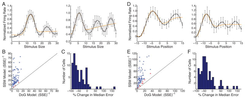
A–C. Periodicity in size-tuning curves (76 cells studied). A. Two example tuning curves, normalized to peak= 1. Data indicates mean ± standard error as determined from maximum likelihood estimation (Supplemental Methods S1.4.2). Curves: best fit Difference of Gaussians (DOG, orange) and Sinusoidal Surround Modulation (SSM, black) models. Tuning curves for all cells: Supplemental Fig. S10. B. Reciprocal of sum squared error (SSE) for DoG and SSM models for all neurons studied. Blue points (73 cells): SSM fit significantly better (p < 0.01) than DoG fit by nested F-test. Red points (3 cells): p > 0.01. C. Cross-validation (c-v) analysis. Histogram of number of cells showing given % change in median sum-squared error (in predicting withheld data, across 100 c-v trials) for SSM model relative to DOG model. D–F. Periodicity in position-tuning curves (74 cells). Conventions and statistical tests as in A–C. D. Two example tuning curves. Tuning curves for all cells: Supplemental Fig. S11. E. Reciprocal of SSE for DoG and SSM models. 66 of 74 cells were significantly better fit by SSM model (blue points). F. C-v analysis. Details of statistical tests for all cells: Supplemental Tables S1–S3 and Text S1.5.2.

We next tested spatial periodicity of the activity profile across the cortical surface for high-contrast stimuli, an issue not previously studied to our knowledge (Fig. 4D–F). Ideally one would show a large drifting grating and sample responses of cells at multiple spatial positions. Instead, we studied the response of each single cell as we moved the drifting grating to multiple randomly interleaved spatial positions. These positional tuning curves showed clear periodicity (Fig. 4D), with 66 of 74 better fit by the SSM than the DOG model (p < 0.01, nested F test; Fig. 4E). In the cross-validation test (Fig. 4F), SSM errors were less than DoG errors for 61 of 74 cells (p = 1.4 × 10⁻⁸, binomial test as above; median significantly different from zero, p = 2.4 × 10⁻⁷, Wilcoxon test as above). This result is particularly surprising given an expectation that receptive field strengths monotonically decrease with distance from their center.

Modeling and Experimental Test II: Contrast Dependence of Net-work Frequency

The model predicts that the network resonant spatial frequencies should increase with contrast (Fig. 3). Such a frequency increase would provide strong evidence that the periodic behaviors are emergent properties of the network dynamics rather than fixed properties of the connections. Because we expected difficulty in accurately measuring oscillations in tuning curves from responses to very low contrast stimuli, we employed a different stimulus used by Tanaka and Ohzawa (2009) to probe center-surround receptive field structure in cat V1: a contrast-modulated sinusoidal grating.

For a given neuron, Tanaka and Ohzawa (2009) presented a large drifting luminance grating covering center and surround, with orientation and spatial frequency (SF) optimal for the CRF, and superimposed a drifting sinusoidal contrast modulation (CM) (Fig. 5A, top). They studied selectivity of the neuron’s response to the CM orientation and SF. The neurons were quite selective, with CM preferred spatial period larger than the period of the CRF’s preferred luminance spatial frequency (mean±sd: 2.1±0.9 times larger) and CM preferred orientations widely distributed relative to CRF preferred orientation.

We model the contrast modulation as spatial periodicity in the input to cortex, i.e. high- or low-contrast regions receive strong or weak input, respectively (Fig. 5A, bottom). The linear model shows CM tuning with preferred spatial period equal to the period of the resonant network activity, i.e. the optimal CM stimulus drives the peaks but not troughs of resonant activity (Fig. 5B,C; Supplemental Fig. S2a,b and Text S2.1). This remains true in the nonlinear model, in which the CM preferred SF, like the other measures of network frequency, increases with stimulus contrast (Fig. 5D; Supplemental Fig. S2e and Text S2.3). Thus, the CM preferred frequency provides an excellent and direct assay of the network’s resonant frequency.

We tested the prediction that network resonant frequencies increase with contrast by studying the contrast dependence of CM preferred SFs, previously measured only at high contrasts (Tanaka and Ohzawa, 2009). 50 cells were studied at four luminance contrasts. Tuning curves for three example cells (Fig. 5E) showed low-pass behavior at low contrast but preference for higher frequencies at higher contrasts. 50% of cells, like these cells, preferred the lowest frequency tested at the lowest contrast tested, whereas none preferred the lowest frequency at the highest contrast tested. The mean CM preferred SF across cells increased significantly with increasing contrast (Fig. 5F). The CM frequency preferred at the lowest contrast tested was lower than at the highest contrast for 72% of cells, the same for 12%, and higher for 16% (Fig. 5G; p = 2.5 × 10⁻⁵ (ties discarded) or p = 9.0 × 10⁻⁵ (ties divided equally), two-sided binomial test assuming “lower” or “higher” equally likely for each cell). We were also able to study length tuning across multiple contrasts in a small number of cells (N = 16), with results consistent with model predictions (Supplemental Fig. S9a–c).

All three experimental measures of network periodicity – length tuning period, position tuning period, and preferred CM SF – have periods, for high contrasts, dominantly in the range 1 to 8 times larger than the period of the CRF’s preferred luminance SF (Fig. 5H–J, and Tanaka and Ohzawa, 2009 for CM SF). This is predicted by the model under a simple heuristic argument: a neuron’s summation field should fill no more than 1/2 cycle of the resonant spatial period, as a larger size would drive suppressive troughs; while empirically, the high-contrast summation field typically contains 0.5–4 CRF preferred luminance spatial periods (Teichert et al., 2007). This argument is supported by our data, as illustrated for size-tuning period (Fig. 5H): mean and median summation field sizes are ≈ 1/2 of the size-tuning period; and summation fields contain 0.5–4 luminance spatial periods. The three different periods are not correlated across cells, neither in experiments nor in a model with stochastic connectivity presented below in Fig. 6 (Supplemental Fig. S9d–e). This presumably reflects different local subnetworks of cells being recruited by each experimental paradigm.

Full Model

Thus far we have studied feature (orientation) effects and spatial effects in separate 1D models. Here we show that these results can all arise in a single model of a large 2D patch of V1, and also consider effects of more realistic stochasticity. Visual position changes smoothly across the 2D patch and units have preferred orientations given by a superposed orientation map (Fig. 6A). Connections and each unit’s parameters are chosen stochastically (which indicates that results are robust to parameter variations), with probability of a connection between two units of given types 0.1 (E projections) or 0.5 (I projections) times the product of unit-height Gaussian functions of positional distance (qualitatively as in Figs. 2–3) and of preferred orientation difference (as in Fig. 1). Dependence of connectivity on preferred orientations is supported by evidence discussed for Fig. 1 and the fact that long-range horizontal excitatory connections preferentially connect neurons of similar preferred orientation (Gilbert and Wiesel, 1989). We have not tried to tune the model other than to find a regime with reasonable surround suppression (and in retrospect the chosen regime may be sub-optimal, Supplemental Methods S1.3.2). Our intent is simply to address qualitative results.

The model qualitatively reproduces all of the results of the previous 1D models, but with more realistic variability. With increasing stimulus strength: (i) input shifts from externally-to network-driven (Fig. 6B) with network input increasingly inhibition-dominated (Fig. 6C), as in Figs. 1E–F and 3A–B; (ii) response summation switches from supralinear to sublinear (Fig. 6D), as in Fig. 1I; (iii) surround suppression and periodicity in length-tuning curves develop (Fig. 6E, average high-strength tuning curves; Fig. 6F, sampling of diverse tuning curves of individual units across input strengths) and summation fields shrink (Fig. 6G), as in Figs. 3C,D. For weak center input strength, surround suppression weakens, and for smaller surrounds can switch to surround facilitation (Fig. 6H), as in Fig. 3E. The periodicity in both length- and position-tuning curves is statistically significant (Fig. 6I), as in the experimental data (Fig. 4B,E). Preferred CM SF increases with stimulus strength (Fig. 6J), as in model and experiment (Fig. 5D–G). Note that preferred CM SF for I units is uniformly 0 for smaller stimulus strengths, consistent with the linear model prediction that a nonzero I-unit resonant spatial frequency requires an ISN (Supplemental Text S2.1.1).

The model also reveals new results. There is no correlation between luminance and CM preferred orientations (Fig. 7A), as in experiments (Tanaka and Ohzawa, 2009). This is because CM preferred orientation arises as a network effect (the best orientation across 2D cortical space of the spatially periodic activity, determined in the model by random variations in intracortical connections), whereas CRF preferred orientation is the luminance orientation that best drives a cell’s external input. The model shows a relatively broad distribution of surround suppression indices, akin to the variability observed experimentally (e.g., Walker et al., 2000) (Fig. 7B), and of I-unit summation field sizes (Fig. 7C), with I units having larger mean summation fields and weaker mean surround suppression than E units, as in Figs. 2B–C, 3C. Surround suppression is tuned for surround orientation (Fig. 7D), with tuning that is weaker for a low-contrast vs. high contrast center (Fig. 7E), both as observed in V1 (Cavanaugh et al., 2002b; Ozeki et al., 2009; Sengpiel et al., 1997).

Figure 7. Two-dimensional probabilistic model: Further results.

A. Histograms of differences between preferred luminance and CM orientations for E (red) and I (blue) units of Fig. 6J for c = 40. The two preferred orientations were completely uncorrelated (E units: r = 0.098, p = 0.33; I units: r = 0.093, p = 0.36). B. Distribution of SSI (see legend of Fig. 6E) for E (red) and I (blue, shown above E) units at 500 randomly selected sites of Fig. 6E. SSI= 0, no suppression; SSI= 1, complete response suppression; SSI< 0, response facilitation. Mean±stdev: E units 0.75±0.18, I units 0.30±0.35. C. Distribution of summation field sizes, same 500 E and 500 I units and colors as B. Mean±stdev: E, 1.08° ± 0.18°; I, 4.97° ± 3.74°. D. Dependence of surround suppression on surround orientation for stimulus strength c = 40. Center stimulus at unit’s preferred orientation fills summation field; surround at varying orientations relative to center stimulus (x-axis) extends stimulus to total diameter 15.1° (70 grid spacings). Mean (solid lines) ± 1 standard deviation (shaded region) of responses of 50 randomly selected E (top) or I (bottom) units each normalized to response to center stimulus alone. E. Orientation tuning of surround suppression decreases for low-strength center. Histograms show circular variances (C.V.’s) of 1 minus the normalized orientation tuning curves of surround suppression (as in D) for the 50 E and 50 I units of D, for center c = 40 (top) or c = 10 (bottom); surround c = 40 in both conditions. Mean C.V. (x̄ in figure) increases significantly at low center strength, indicating broader orientation tuning. Mean±stdev of C.V.’s for high (c = 40) and low (c = 10) contrast and p values for difference between two distributions using 2-sided Wilcoxon rank sum test: All units: high 0.64 ± 0.11, low 0.74 ± 0.11, p = 2.6 × 10⁻⁹; E units: high 0.62 ± 0.10, low 0.77 ± 0.09, p = 6.3 × 10⁻¹⁰; I units: high 0.67 ± 0.12, low 0.72 ± 0.12, p = 0.034.

Discussion

The stabilized supralinear network (SSN) provides a remarkably simple account, and the first unifying circuit account, of a wide variety of behaviors across multiple cortical areas. These include surround suppression, normalization, and their dependencies on contrast and other stimulus parameters (see multiple references in Introduction), as well as spatial periodicity in activity and length-tuning (Anderson et al., 2001; Tanaka and Ohzawa, 2009; Wang et al., 2009). The model requires no fine tuning, producing qualitatively similar behavior over broad parameter regimes. Our first experimental tests provide strong support, for the first time demonstrating systematic periodicity in high-contrast length-tuning and position-tuning curves (the latter indirectly indicating spatial periodicity in activity) as well as an increase in the underlying spatial frequency of periodic activity with increasing contrast as measured by CM preferred spatial frequency.

The model depends on very few assumptions, most importantly a supralinear I/O function for single neurons and sufficiently strong recurrent excitation and feedback inhibition. It differs from previous circuit models (e.g., Schwabe et al., 2010; Somers et al., 1998, and models reviewed in Carandini and Heeger, 2012) in providing a unified network explanation of multiple aspects of both contextual modulation and normalization, exhibiting similar behaviors for both E and I cells, showing suppression and normalization without increases in inhibition, and explaining contrast-dependent behaviors without assuming a class of inhibitory neurons that are ineffective at lower contrasts.

Connection to the balanced network

As discussed in more detail in Ahmadian et al. (2013), in both the SSN and the balanced network model (van Vreeswijk and Sompolinsky, 1998), the dynamics robustly lead inhibition to stabilize excitation. However, the two models operate in very different regimes. In the balanced network, both external and network-driven inputs are very large but are tightly balanced, leaving only a far smaller residual input. This predicts external input alone is much larger than net input, counter to results of isolating external input by silencing cortex (e.g. Priebe and Ferster, 2008). Due to tight balancing, the balanced network can only respond linearly to the input. In the SSN, inputs are not large, the balance is loose, and nonlinear behavior like that seen in cortex can result. In preliminary results with spiking models, SSN behavior is reproduced while, like the balanced network, producing asynchronous, irregular firing (D. Obeid and K.D. Miller, unpublished).

Experimental Predictions

The model makes many experimental predictions beyond those we tested: (1) For linearly adding external inputs, cortical areas should show supralinear (weak input) or sublinear (strong input) response summation; optogenetically stimulating two distinct sets of neurons could ensure linear input addition. (2) & (3): Periodicity in length- and positional-tuning should (2) decrease in wavelength with increasing contrast, as shown here for CM tuning, and 3) attenuate or disappear as stimuli are changed from sharp-edged to slowly tapering, while CM tuning persists. (4) & (5): Across a variety of normalization or suppression phenomena, (4) E and I cells should show similar behavior (both normalized or both suppressed). However, this may be confounded by multiple inhibitory subtypes with differing responses, so a more robust prediction (Supplemental Text S2.2.3) is (5) response suppression in E cells should be accompanied by a decrease in the I conductance they receive. (6) The summation field for directional tuning in MT should shrink with contrast.

A seventh prediction is that ISN behavior should occur only for lower spatial frequencies of input to I cells along with sufficient network activation to drive the network into the ISN regime (Supplemental Text S2.2). A key ISN behavior is the “paradoxical” response of I cells: addition of excitatory drive to I cells causes them to lower their firing rates in the new steady state (Ozeki et al., 2009; Tsodyks et al., 1997). Thus, if channelrhodopsin-2 (ChRh2) were expressed in I neurons, and a light pattern of a given spatial frequency were modulated or drifted at low temporal frequency while a visual stimulus was presented, the network should show paradoxical response only for sufficient visual contrast and then only for spatial frequencies of light below a critical frequency k_cr (Fig. 8). This predicts a sharp jump, with increasing spatial frequency, of about 180° in the relative phase of E and I cell activities as k_cr is crossed, or more robustly (Supplemental Text S2.2.3), in the relative phases of the E and I conductances received by excitatory cells.

Figure 8. Spatial-frequency- and contrast-dependent paradoxical response in the 2-dimensional nonlinear model.

Slowly drifting, spatially sinusoidal modulatory input is given to I units (e.g., by photostimulation with ChRh2 expressed in I cells), in the presence of varying levels of spatially uniform tonic visual input driving both E and I units. “Paradoxical” ISN behavior –I firing rates decreasing for increased input to I units – manifests as E and I units modulating in phase with one another. For weak tonic input, the network is a non-ISN and units respond non-paradoxically (input and I in phase, E at opposite phase) for all modulatory spatial frequencies. For high tonic input, network is an ISN. Then low-spatial-frequency, but not high-spatial-frequency modulation drives units paradoxically (Supplemental Text S2.2 and Supplemental Fig. S2c). A more robust prediction is that these changes in relative phase will occur in the excitation and inhibition received by cells (Supplemental Text S2.2.3). Input and E and I firing rates are all shown normalized to both their minimum and maximum values.

We also note several caveats. In some species or areas spontaneous activity may suffice to drive the network out of the supralinearly summating regime. Periodicity in length-and position-tuning curves depends on sharp-edged input, but this might not correspond directly to stimulus shape: connection fan-in and fan-out at previous stages could spatially smooth input from sharp-edged stimuli, while processing (e.g., surround suppression) at previous stages could sharpen input edges for smoothly tapering stimuli. Because I cells have wider summation fields than E cells, intermediate stimulus sizes can suppress E cells but facilitate I cells (see Discussion of results of Haider et al., 2010, below). In parameter regimes in which I projections are not too narrow, both E and I cells can be surround suppressed with increases in the inhibition they receive: inhibition from new I cells recruited by a larger stimulus can outweigh loss of inhibition from suppressed I cells. Other factors that can dynamically change effective synaptic strengths – short-term synaptic depression or facilitation, adaptation currents – may add complexity to model behavior, but will not alter the basic SSN distinction between weak- and strong-effective-synapse regimes.

Does the SSN model apply to rodent cortex?

We have primarily modeled data from species with columnar organization and maps of features such as preferred orientation. Does our model apply to species, such as rodents, that lack such organization?

Recurrent excitation in rodents may be weaker than in species with columnar organization, so that excitatory instability and the transition to sublinear behavior may not occur. This is suggested by results of Atallah et al. (2012) in mouse V1 L2/3: optogenetic suppression of parvalbumin (PV)-expressing I cells increased E-cell visual responses without any increase in the excitatory conductance they received and with a non-paradoxical increase in inhibitory conductance, suggesting a dearth of E→E coupling and non-ISN behavior. This could explain why maps fail to develop in rodents, as such failure can occur if local interactions between neurons are suppressive (Kaschube, 2014). However, engagement of L2/3 excitatory connectivity may vary with experimental conditions or area. In rodent auditory cortex, locomotion added drive to L1 I neurons, suppressing L2/3 E-cell firing with a paradoxical suppression of inhibitory conductance they received, suggesting an ISN (Zhou et al., 2014). Other results suggest strong recurrent excitation and ISN-like behavior in L5 of rodent cortex (London et al., 2010; Stroh et al., 2013); rodent response properties might be synthesized in deep layers by SSN mechanisms and propagate to upper layers.

Adesnik et al. (2012) found in mouse V1 L2/3 that somatostatin-expressing I cells (SOM cells) were surround facilitated while E and PV cells were suppressed, suggesting a non-ISN in which increased SOM inhibition mediates suppression (Nienborg et al., 2013). However, suppression might decrease the net inhibition (SOM+PV) cells receive, as in an ISN; optogenetic suppression of SOM-cell spiking only moderately reduced E-cell surround suppression; and another study found both SOM and PV neurons were surround suppressed (Pecka et al., 2014). The relative sparsity of SOM cells and increased proportion of PV cells in macaque vs. mouse V1 (reviewed in Nienborg et al., 2013) is another potentially significant species difference.

A conflicting experiment?

The model suggests a resolution to the apparent conflict between two findings: inhibition decreased during surround suppression (Ozeki et al., 2009); yet increased stimulus size in windowed natural movies suppressed E cell firing while increasing the inhibition they receive and PV cell firing (Haider et al., 2010). Haider et al. (2010) used small stimuli: for a given cell, center stimuli had size giving half-maximal response, which for a Gaussian-shaped CRF is about 0.5–0.6× CRF size (Supplemental Methods S1.3.4); large stimuli were three times larger, or 1.5–1.8× CRF size (vs. surrounds typically 10× CRF size in Ozeki et al., 2009). PV cells have larger summation fields than E cells in mice (Adesnik et al., 2012) and our model (Fig. 7C). Thus, Haider et al. (2010)’s larger stimuli (i) to E cells might have size close to optimal for I cells; (ii) to I cells might evoke more response than center stimuli, even if optimal size were in between. Supplemental Fig. S14 shows how the model could simultaneously produce the results of both studies. The broad spatiotemporal power spectrum of natural stimuli may also contribute: paradoxical effects arise only at lower spatial frequencies (Fig. 8) and similar dependence might occur for temporal frequency.

Extension to other cortical properties

The network’s winner-take-all property for unequal-strength inputs may explain suppression of correlated neural variability induced by a sensory stimulus or motor plan (Churchland et al., 2010) or attention (Cohen and Maunsell, 2009; Mitchell et al., 2009): increasing strength of other inputs (stimulus, plan, attention) suppresses the contribution of correlated neural noise to neuronal output. Multiple attentional effects on neural responses arise if attention modulates inputs to a normalizing circuit (e.g. Reynolds and Heeger, 2009); the SSN model is likely to reproduce these effects. Future studies will address these issues.

Attentional enhancement and modulatory suppression can be understood as opposite turns of a “knob” adjusting the gain of “balanced amplification” (Murphy and Miller, 2009), which arises in the ISN regime: a small network shift towards inhibition (e.g. addition of modulatory E input to I cells) causes a large decrease in both E- and I-cell responses, while a small shift toward excitation causes large increases in both (these changes can be multiplicative, i.e. gain changes, in the SSN: Supplemental Fig. S13). Thus, a function of strong cortical recurrence may be to provide modulatable amplification.

Conclusion

The SSN provides a powerful framework for understanding how sensory cortex globally integrates multiple sources of input, bottom-up and top-down, to produce neuronal responses and ultimately perception. The computational function of these integrative behaviors may now be more deeply probed by studying how the underlying circuit processes more complex and natural stimuli. Circuit changes that cause failures of this basic circuit operation might manifest at multiple cortical levels from primary sensation to higher cognition. Understanding such failures may provide insight into disorders such as autism and schizophrenia, which show deficits in contextual (Silverstein and Keane, 2011) or global (Qian and Lipkin, 2011) processing and involve disruptions in E/I balance (Yizhar et al., 2011; Yoon et al., 2010) that could disrupt the balanced amplification underlying SSN modulations. Indeed, schizophrenics show reduced visual surround suppression that correlates with reduced GABA concentration in visual cortex (Yoon et al., 2010), while autistic subjects show increased variability in sensory responses (Dinstein et al., 2012), which might reflect failure of normalization-induced variability suppression.

References

- Adesnik H, Bruns W, Taniguchi H, Huang ZJ, Scanziani M. A neural circuit for spatial summation in visual cortex. Nature. 2012;490:226–231. doi: 10.1038/nature11526. [DOI] [PMC free article] [PubMed] [Google Scholar]
- Adini Y, Sagi D, Tsodyks M. Excitatory-inhibitory network in the visual cortex: psychophysical evidence. Proc Natl Acad Sci U S A. 1997;94:10426–10431. doi: 10.1073/pnas.94.19.10426. [DOI] [PMC free article] [PubMed] [Google Scholar]
- Ahmadian Y, Rubin DB, Miller KD. Analysis of the stabilized supralinear network. Neural Computation. 2013;25:1994–2037. doi: 10.1162/NECO_a_00472. [DOI] [PMC free article] [PubMed] [Google Scholar]
- Anderson JS, Lampl I, Gillespie DC, Ferster D. Membrane potential and conductance changes underlying length tuning of cells in cat primary visual cortex. J Neurosci. 2001;21:2104–2112. doi: 10.1523/JNEUROSCI.21-06-02104.2001. [DOI] [PMC free article] [PubMed] [Google Scholar]
- Atallah BV, Bruns W, Carandini M, Scanziani M. Parvalbumin-expressing interneurons linearly transform cortical responses to visual stimuli. Neuron. 2012;73:159–170. doi: 10.1016/j.neuron.2011.12.013. [DOI] [PMC free article] [PubMed] [Google Scholar]
- Busse L, Wade AR, Carandini M. Representation of concurrent stimuli by population activity in visual cortex. Neuron. 2009;64:931–942. doi: 10.1016/j.neuron.2009.11.004. [DOI] [PMC free article] [PubMed] [Google Scholar]
- Carandini M, Heeger DJ. Normalization as a canonical neural computation. Nat Rev Neurosci. 2012;13:51–62. doi: 10.1038/nrn3136. [DOI] [PMC free article] [PubMed] [Google Scholar]
- Cavanaugh J, Joiner WM, Wurtz RH. Suppressive surrounds of receptive fields in monkey frontal eye field. J Neurosci. 2012;32:12284–12293. doi: 10.1523/JNEUROSCI.0864-12.2012. [DOI] [PMC free article] [PubMed] [Google Scholar]
- Cavanaugh JR, Bair W, Movshon JA. Nature and interaction of signals from the receptive field center and surround in macaque V1 neurons. J Neurophysiol. 2002a;88:2530–2546. doi: 10.1152/jn.00692.2001. [DOI] [PubMed] [Google Scholar]
- Cavanaugh JR, Bair W, Movshon JA. Selectivity and spatial distribution of signals from the receptive field surround in macaque V1 neurons. J Neurophysiol. 2002b;88:2547–2556. doi: 10.1152/jn.00693.2001. [DOI] [PubMed] [Google Scholar]
- Churchland MM, Yu BM, Cunningham JP, Sugrue LP, Cohen MR, Corrado GS, Newsome WT, Clark AM, Hosseini P, Scott BB, et al. Stimulus onset quenches neural variability: a widespread cortical phenomenon. Nat Neurosci. 2010;13:369–378. doi: 10.1038/nn.2501. [DOI] [PMC free article] [PubMed] [Google Scholar]
- Cohen MR, Maunsell JH. Attention improves performance primarily by reducing interneuronal correlations. Nat Neurosci. 2009;12:1594–1600. doi: 10.1038/nn.2439. [DOI] [PMC free article] [PubMed] [Google Scholar]
- Dinstein I, Heeger DJ, Lorenzi L, Minshew NJ, Malach R, Behrmann M. Unreliable evoked responses in autism. Neuron. 2012;75:981–991. doi: 10.1016/j.neuron.2012.07.026. [DOI] [PMC free article] [PubMed] [Google Scholar]
- Ermentrout GB, Terman DH. Mathematical Foundations of Neuroscience. Springer; New York: 2010. [Google Scholar]
- Falkner AL, Krishna BS, Goldberg ME. Surround suppression sharpens the priority map in the lateral intraparietal area. J Neurosci. 2010;30:12787–12797. doi: 10.1523/JNEUROSCI.2327-10.2010. [DOI] [PMC free article] [PubMed] [Google Scholar]
- Gilbert CD, Wiesel TN. Columnar specificity of intrinsic horizontal and cortico-cortical connections in cat visual cortex. J Neurosci. 1989;9:2432–2442. doi: 10.1523/JNEUROSCI.09-07-02432.1989. [DOI] [PMC free article] [PubMed] [Google Scholar]
- Haider B, Krause MR, Duque A, Yu Y, Touryan J, Mazer JA, McCormick DA. Synaptic and network mechanisms of sparse and reliable visual cortical activity during nonclassical receptive field stimulation. Neuron. 2010;65:107–121. doi: 10.1016/j.neuron.2009.12.005. [DOI] [PMC free article] [PubMed] [Google Scholar]
- Hansel D, van Vreeswijk C. How noise contributes to contrast invariance of orientation tuning in cat visual cortex. J Neurosci. 2002;22:5118–5128. doi: 10.1523/JNEUROSCI.22-12-05118.2002. [DOI] [PMC free article] [PubMed] [Google Scholar]
- Heuer HW, Britten KH. Contrast dependence of response normalization in area MT of the rhesus macaque. J Neurophysiol. 2002;88:3398–3408. doi: 10.1152/jn.00255.2002. [DOI] [PubMed] [Google Scholar]
- Kapfer C, Glickfeld L, Atallah B, Scanziani M. Supralinear increase of recurrent inhibition during sparse activity in the somatosensory cortex. Nat Neurosci. 2007;10:743–753. doi: 10.1038/nn1909. [DOI] [PMC free article] [PubMed] [Google Scholar]
- Kaschube M. Neural maps versus salt-and-pepper organization in visual cortex. Curr Opin Neurobiol. 2014;24:95–102. doi: 10.1016/j.conb.2013.08.017. [DOI] [PubMed] [Google Scholar]
- London M, Roth A, Beeren L, Hausser M, Latham PE. Sensitivity to perturbations in vivo implies high noise and suggests rate coding in cortex. Nature. 2010;466:123–127. doi: 10.1038/nature09086. [DOI] [PMC free article] [PubMed] [Google Scholar]
- MacEvoy SP, Tucker TR, Fitzpatrick D. A precise form of divisive suppression supports population coding in the primary visual cortex. Nat Neurosci. 2009;12:637–645. doi: 10.1038/nn.2310. [DOI] [PMC free article] [PubMed] [Google Scholar]
- Marino J, Schummers J, Lyon DC, Schwabe L, Beck O, Wiesing P, Obermayer K, Sur M. Invariant computations in local cortical networks with balanced excitation and inhibition. Nature Neurosci. 2005;8:194–201. doi: 10.1038/nn1391. [DOI] [PubMed] [Google Scholar]
- Miller KD, Troyer TW. Neural noise can explain expansive, power-law nonlinearities in neural response functions. J Neurophysiol. 2002;87:653–659. doi: 10.1152/jn.00425.2001. [DOI] [PubMed] [Google Scholar]
- Mitchell JF, Sundberg KA, Reynolds JH. Spatial attention decorrelates intrinsic activity fluctuations in macaque area V4. Neuron. 2009;63:879–888. doi: 10.1016/j.neuron.2009.09.013. [DOI] [PMC free article] [PubMed] [Google Scholar]
- Murphy BK, Miller KD. Balanced amplification: A new mechanism of selective amplification of neural activity patterns. Neuron. 2009;61:635–648. doi: 10.1016/j.neuron.2009.02.005. [DOI] [PMC free article] [PubMed] [Google Scholar]
- Nienborg H, Hasenstaub A, Nauhaus I, Taniguchi H, Huang ZJ, Callaway EM. Contrast dependence and differential contributions from somatostatin-and parvalbumin-expressing neurons to spatial integration in mouse V1. J Neurosci. 2013;33:11145–11154. doi: 10.1523/JNEUROSCI.5320-12.2013. [DOI] [PMC free article] [PubMed] [Google Scholar]
- Ozeki H, Finn IM, Schaffer ES, Miller KD, Ferster D. Inhibitory stabilization of the cortical network underlies visual surround suppression. Neuron. 2009;62:578–592. doi: 10.1016/j.neuron.2009.03.028. [DOI] [PMC free article] [PubMed] [Google Scholar]
- Pecka M, Han Y, Sader E, Mrsic-Flogel TD. Experience-Dependent Specialization of Receptive Field Surround for Selective Coding of Natural Scenes. Neuron. 2014;84:457–469. doi: 10.1016/j.neuron.2014.09.010. [DOI] [PMC free article] [PubMed] [Google Scholar]
- Priebe NJ, Ferster D. Inhibition, spike threshold and stimulus selectivity in primary visual cortex. Neuron. 2008;57:482–497. doi: 10.1016/j.neuron.2008.02.005. [DOI] [PubMed] [Google Scholar]
- Qian N, Lipkin RM. A learning-style theory for understanding autistic behaviors. Front Hum Neurosci. 2011;5:77. doi: 10.3389/fnhum.2011.00077. [DOI] [PMC free article] [PubMed] [Google Scholar]
- Reynolds JH, Heeger DJ. The normalization model of attention. Neuron. 2009;61:168–185. doi: 10.1016/j.neuron.2009.01.002. [DOI] [PMC free article] [PubMed] [Google Scholar]
- Sachdev RN, Krause MR, Mazer JA. Surround suppression and sparse coding in visual and barrel cortices. Front Neural Circuits. 2012;6:43. doi: 10.3389/fncir.2012.00043. [DOI] [PMC free article] [PubMed] [Google Scholar]
- Sceniak M, Ringach DL, Hawken M, Shapley R. Contrast’s effect on spatial summation by macaque v1 neurons. Nature Neurosci. 1999;2:733–739. doi: 10.1038/11197. [DOI] [PubMed] [Google Scholar]
- Schwabe L, Ichida JM, Shushruth S, Mangapathy P, Angelucci A. Contrast-dependence of surround suppression in Macaque V1: experimental testing of a recurrent network model. Neuroimage. 2010;52:777–792. doi: 10.1016/j.neuroimage.2010.01.032. [DOI] [PMC free article] [PubMed] [Google Scholar]
- Sengpiel F, Blakemore C, Sen A. Characteristics of surround inhibition in cat area 17. Exp Brain Res. 1997;116:216–228. doi: 10.1007/pl00005751. [DOI] [PubMed] [Google Scholar]
- Sengpiel F, Vorobyov V. Intracortical origins of interocular suppression in the visual cortex. J Neurosci. 2005;25:6394–6400. doi: 10.1523/JNEUROSCI.0862-05.2005. [DOI] [PMC free article] [PubMed] [Google Scholar]
- Shao YR, Isett BR, Miyashita T, Chung J, Pourzia O, Gasperini RJ, Feldman DE. Plasticity of recurrent l2/3 inhibition and gamma oscillations by whisker experience. Neuron. 2013;80:210–222. doi: 10.1016/j.neuron.2013.07.026. [DOI] [PMC free article] [PubMed] [Google Scholar]
- Shushruth S, Ichida JM, Levitt JB, Angelucci A. Comparison of spatial summation properties of neurons in macaque V1 and V2. J Neurophysiol. 2009;102:2069–2083. doi: 10.1152/jn.00512.2009. [DOI] [PMC free article] [PubMed] [Google Scholar]
- Silverstein SM, Keane BP. Perceptual organization impairment in schizophrenia and associated brain mechanisms: review of research from 2005 to 2010. Schizophr Bull. 2011;37(4):690–699. doi: 10.1093/schbul/sbr052. [DOI] [PMC free article] [PubMed] [Google Scholar]
- Somers D, Todorov E, Siapas A, Toth L, Kim D, Sur M. A local circuit approach to understanding integration of long-range inputs in primary visual cortex. Cereb Cortex. 1998;8:204–217. doi: 10.1093/cercor/8.3.204. [DOI] [PubMed] [Google Scholar]
- Song XM, Li CY. Contrast-dependent and contrast-independent spatial summation of primary visual cortical neurons of the cat. Cerebral Cortex. 2008;18:331–336. doi: 10.1093/cercor/bhm057. [DOI] [PubMed] [Google Scholar]
- Stroh A, Adelsberger H, Groh A, Ruhlmann C, Fischer S, Schierloh A, Deisseroth K, Konnerth A. Making waves: initiation and propagation of corticothalamic Ca2+ waves in vivo. Neuron. 2013;77:1136–1150. doi: 10.1016/j.neuron.2013.01.031. [DOI] [PubMed] [Google Scholar]
- Sundberg KA, Mitchell JF, Reynolds JH. Spatial attention modulates center-surround interactions in macaque visual area v4. Neuron. 2009;61:952–963. doi: 10.1016/j.neuron.2009.02.023. [DOI] [PMC free article] [PubMed] [Google Scholar]
- Tanaka H, Ohzawa I. Surround suppression of V1 neurons mediates orientation-based representation of high-order visual features. J Neurophysiol. 2009;101:1444–1462. doi: 10.1152/jn.90749.2008. [DOI] [PubMed] [Google Scholar]
- Teichert T, Wachtler T, Michler F, Gail A, Eckhorn R. Scale-invariance of receptive field properties in primary visual cortex. BMC Neurosci. 2007;8:38. doi: 10.1186/1471-2202-8-38. [DOI] [PMC free article] [PubMed] [Google Scholar]
- Tsodyks MV, Skaggs WE, Sejnowski TJ, McNaughton BL. Paradoxical effects of external modulation of inhibitory interneurons. J Neurosci. 1997;17:4382–4388. doi: 10.1523/JNEUROSCI.17-11-04382.1997. [DOI] [PMC free article] [PubMed] [Google Scholar]
- Tsui JM, Pack CC. Contrast sensitivity of MT receptive field centers and surrounds. J Neurophysiol. 2011;106:1888–1900. doi: 10.1152/jn.00165.2011. [DOI] [PubMed] [Google Scholar]
- Van den Bergh G, Zhang B, Arckens L, Chino YM. Receptive-field properties of V1 and V2 neurons in mice and macaque monkeys. J Comp Neurol. 2010;518:2051–2070. doi: 10.1002/cne.22321. [DOI] [PMC free article] [PubMed] [Google Scholar]
- van Vreeswijk C, Sompolinsky H. Chaotic balanced state in a model of cortical circuits. Neural Computation. 1998;10:1321–1371. doi: 10.1162/089976698300017214. [DOI] [PubMed] [Google Scholar]
- Vanni MP, Casanova C. Surround suppression maps in the cat primary visual cortex. Front Neural Circuits. 2013;7:78. doi: 10.3389/fncir.2013.00078. [DOI] [PMC free article] [PubMed] [Google Scholar]
- Walker G, Ohzawa I, Freeman R. Suppression outside the classical cortical receptive field. Vis Neurosci. 2000;17:369–379. doi: 10.1017/s0952523800173055. [DOI] [PubMed] [Google Scholar]
- Wang C, Bardy C, Huang JY, FitzGibbon T, Dreher B. Contrast dependence of center and surround integration in primary visual cortex of the cat. J Vis. 2009;9:1–15. doi: 10.1167/9.1.20. [DOI] [PubMed] [Google Scholar]
- Yizhar O, Fenno LE, Prigge M, Schneider F, Davidson TJ, O’Shea DJ, Sohal VS, Goshen I, Finkelstein J, Paz JT, et al. Neocortical excitation/inhibition balance in information processing and social dysfunction. Nature. 2011;477:171–178. doi: 10.1038/nature10360. [DOI] [PMC free article] [PubMed] [Google Scholar]
- Yoon JH, Maddock RJ, Rokem A, Silver MA, Minzenberg MJ, Ragland JD, Carter CS. GABA concentration is reduced in visual cortex in schizophrenia and correlates with orientation-specific surround suppression. J Neurosci. 2010;30:3777–3781. doi: 10.1523/JNEUROSCI.6158-09.2010. [DOI] [PMC free article] [PubMed] [Google Scholar]
- Zhou M, Liang F, Xiong XR, Li L, Li H, Xiao Z, Tao HW, Zhang LI. Scaling down of balanced excitation and inhibition by active behavioral states in auditory cortex. Nat Neurosci. 2014;17:841–850. doi: 10.1038/nn.3701. [DOI] [PMC free article] [PubMed] [Google Scholar]
Associated Data
This section collects any data citations, data availability statements, or supplementary materials included in this article.