Exact milestoning

Abstract

A new theory and an exact computer algorithm for calculating kinetics and thermodynamic properties of a particle system are described. The algorithm avoids trapping in metastable states, which are typical challenges for Molecular Dynamics (MD) simulations on rough energy landscapes. It is based on the division of the full space into Voronoi cells. Prior knowledge or coarse sampling of space points provides the centers of the Voronoi cells. Short time trajectories are computed between the boundaries of the cells that we call milestones and are used to determine fluxes at the milestones. The flux function, an essential component of the new theory, provides a complete description of the statistical mechanics of the system at the resolution of the milestones. We illustrate the accuracy and efficiency of the exact Milestoning approach by comparing numerical results obtained on a model system using exact Milestoning with the results of long trajectories and with a solution of the corresponding Fokker-Planck equation. The theory uses an equation that resembles the approximate Milestoning method that was introduced in 2004 [A. K. Faradjian and R. Elber, J. Chem. Phys. 120(23), 10880-10889 (2004)]. However, the current formulation is exact and is still significantly more efficient than straightforward MD simulations on the system studied.

I. INTRODUCTION

The Molecular Dynamics (MD) method is a useful tool for studying properties of matter with atomically detailed simulations. MD makes it possible to connect microscopic structures and interactions with thermodynamics, kinetics, and mechanisms of molecular processes. Nevertheless, a significant limitation of these simulations is that of time scales. The fundamental numerical time step (∼10⁻¹⁵ s) is much shorter than many observation times in biophysics, for example, enzymatic reactions can take milliseconds and longer. This limitation makes MD simulations for these systems extremely expensive. While considerable progress in extending time scales of MD was made by improvements in specialized and general hardware,¹ significant limitations remain on the length of a single trajectory (microseconds for readily accessible machines) and on generating an ensemble of long trajectories necessary for estimating kinetics. Methods to speed up these calculations are desired.

Why are so many time steps required when the spatial reorganization of the molecules that we examine is frequently small? MD simulations can be long because a significant fraction of the time the system is located at metastable states or deep free energy minima. Nothing much happened while the system diffuse in the metastable state. Shortening the wait time at the metastable states while still retaining the correctness of the sampling and time scales is a prime motivation behind the exact Milestoning algorithm. We comment that in many biomolecular systems, the number of metastable states can be very large. In general, it is not sufficient to use a two state system (reactant and product) as an effective description of complex dynamics. In many biophysical systems, it is necessary to consider a truly rough energy landscape with almost a continuum of temporal and spatial scales. A classic example is the study of myoglobin.² Appropriate technologies for such complex systems are desired.

Indeed, a number of different theoretical and algorithmic approaches aim to extend the time scale of simulations and produce trajectories probing slow kinetics. Notable methods are action-based approaches. In this class of techniques, trajectories of time scales much longer than temporal ranges accessible to MD are estimated.³ Other approaches⁴ are aimed at sampling trajectories that pass over a few significant energy barriers. Individual trajectories in the latter case are not long in time but are rare and therefore the average process is slow. On rough energy landscapes, in which we find numerous metastable states, broad distributions of barrier heights, and wide range of minimum depths, individual trajectories may be long in time. Technologies based on short and rare trajectories are difficult to use in a straightforward fashion in these systems. This is since individual trajectories between reactants and products can be long (the trajectories may be trapped for a long time in metastable states that are not the initial or the final states). Hence, kinetics may not be sampled properly by rare (and short) trajectory strategies. Methods like replica exchange transition interface sampling⁵ aimed to enhance sampling by identifying the metastable states and focusing on the transitions between the metastable states using short trajectories. The number of these metastable states and the complexity of characterizing them can grow exponentially with the system size.⁶ Studies of such systems are a significant challenge, and an efficient algorithm to enumerate them is not known. It is desired to develop a technique that enhances the time scale of simulations and is less sensitive to the features of the underlying energy landscape.

Approaches like PPTIS (Partial Paths Transition Interface Sampling),⁷ Weighted Ensemble (WE),⁸ and Milestoning⁹ aim to address the last problem and consider dynamics that can be a mix of diffusive (small barrier) and activated (large barrier) processes. Designing the method with rough energy landscapes in mind leads to technologies that are less impacted by the broad distributions of barriers and minima we frequently encounter in molecular biophysics¹⁰ or the “small barrier” problem of material science.¹¹ Both PPTIS and Milestoning were introduced as highly efficient and approximate methods, while WE is in principle exact for stochastic dynamics. PPTIS and Milestoning exploit the use of short trajectory fragments to estimate a local kinetic operator. The operator is then used in probabilistic modeling of longer time scales.

The purpose of the present manuscript is to formulate and illustrate an exact Milestoning approach. It offers an exact description of the statistical mechanics of the system while retaining many of the useful features of the original approximate algorithm.¹² The theory was tested and illustrated extensively in the past (see, for instance, Refs. 13 and 14) and a review is available.¹² Nevertheless, since the theory and implementation have evolved considerably and are now exact, we repeat and redefine some of the concepts that were introduced earlier in the formulation of Faradjian and Elber⁹ and Kirmizialtin and Elber.¹² The current formulation also builds on the Voronoi tessellation of Markovian Milestoning introduced by Venturoli and Vanden-Eijnden¹⁵ and adjusted to avoid milestone crossing by Majek and Elber.¹⁶ Finally, the idea of exact molecular dynamics trajectories through interfaces was discussed in a more limited fashion in earlier works by Warmflash, Bhimalapuram, and Dinner and in a follow up paper by Dickson, Warmflash, and Dinner.^17,18 It was also examined by Vanden-Eijnden and Venturoli in their trajectory tilting approach.¹⁹ These studies did not offer a complete statistical mechanical view, which is offered by the approach of exact Milestoning.

Compared to weighted ensemble, another method that is statistically exact,⁸ Milestoning is more flexible in the choice of the dynamics. The WE approach requires stochastic equations of motion to allow splitting and termination of trajectories. Milestoning uses stochastic considerations only to determine initial conditions and can use straightforward and deterministic equations such as Hamilton equations. The exact Milestoning algorithm can be applied to non-equilibrium cases.

This manuscript is organized as follows. In Sec. II, we motivate the study and present the general principles of exact Milestoning and the corresponding algorithms. More specifically, we start with the definition of the milestones (Sec. II A), continue to define the core equations for the probability of crossing a milestone and of the absolute flux (Sec. II B), derive the formula for the stationary flux, a core entity of the Milestoning theory (Sec. II C), discuss the algorithm to compute the stationary flux (Sec. II D), consider the probabilities of the states (Sec. II E), and finally examine moments of the distribution of the first passage time (Sec. II F). In Sec. III, we consider a numerical example. In Sec. III A, we describe the simple two-dimensional energy surface that we use for illustration. The type of the dynamics (Brownian) is described in Sec. III B. The results and discussion are in Sec. IV. In Sec. IV A, we consider numerical calculations of the stationary flux and the MFPT (Mean First Passage Time) using exact Milestoning. In Sec. IV B, we solve the same problem using the Fokker-Planck equation (FPE). In Sec. IV C, we compare exact Milestoning and the FPE solutions. In Sec. IV D, we compare the exact Milestoning calculations to a calculation based on very long trajectories (the most straightforward approach for this type of problem in systems with a large number of degrees of freedom) and discuss accuracy and efficiency. In Sec. IV E, we examine the rate of convergence as a function of the initial guess and illustrate that starting from equilibrium distributions at the milestones is significantly more efficient than initiating the system at one milestone. The summary of the paper is in Sec. V.

II. THEORY AND CALCULATIONS

A. Definition and the choice of the milestones

A system of N particles at time t is fully characterized by a phase space vector, $x\left(t\right)$.

We are given a set of points (in phase or coordinate spaces), ${\left\{x_i\right\}}_{i=1}^L$, which we call anchors. These points guide the trajectory calculations and establish centers of Voronoi cells, which were introduced to Milestoning by Vanden-Eijnden and Venturoli.¹⁵ A Voronoi cell j is defined as the set of all points x such that their distance to x_j is shorter than a distance to any other anchor, $x_k\left(k\ne j\right)$. A dividing surface between two cells, i and j, which we call a milestone, is the set of all points x such that their distances from i and j is the same and smaller than the distance to any other anchor. For example, if the anchor points form a straight line in a two-dimensional space, the milestones would be orthogonal lines exactly between the anchors. A trajectory may cross a milestone and transition between two Voronoi cells. Crossing a milestone is the fundamental event in the theory of Milestoning and a state is defined by the last milestone that was crossed. We denote milestones by M_α where the index α is a shortcut for a pair of anchors, say, ij. The total number of milestones is M.

How do we obtain the initial set of anchors? There are numerous ways of obtaining them. In the past, we have used our algorithms for reaction path calculations^21,22 to determine points along a reaction coordinate and to conduct Milestoning calculations in one dimension.^14,23,24 In other studies, we have used chemical intuition to determine relevant sample coordinates for protein folding (backbone torsions),²⁵ pick up structure from replica exchange equilibrium calculations,²⁶ or even use a field representation of material density.²⁷ Hence, the choice of anchors is highly flexible, and we rely on the user to provide a sensible sample of anchors that can (a) describe the process of interest as a sequence of transitions between cells associated with the anchors and that (b) the transitions between cells can be effectively sampled by short trajectories. While we have not emphasized this point in the past, the set of anchors can be adjusted dynamically. As we explore more phase space points using trajectories between interfaces, we may discover new portions of phase space that require sampling and therefore new anchors can be generated on the fly.

There is also considerable flexibility in the definition of the distances mentioned above. In the present discussion, the distance between any two points, x_i and x_j, is simply $d_{ij}=\sqrt{{\left(x_i-x_j\right)}^t\left(x_i-x_j\right)}$. However, the distance can be defined also in coarse space. Let a vector of coordinates in coarse space be $Q\left(x\right)Q\in R^J$, where J < 3N. The distance in coarse space is $d_{Q,ij}=\sqrt{{\left(Q_i-Q_j\right)}^t\left(Q_i-Q_j\right)}$. For example, when describing protein folding, the coordinates of the protein and not of the solvent are likely to be sufficient to describe the reaction. Of course, the dynamics is still conducted in the full space of $x\left(t\right)$.

B. Definitions: Space of events, probability of events, flux, and kernel

1. Definitions

Milestoning events: The basic event of the statistical theory for kinetics and thermodynamics is the last crossing of a milestone (say, α) by a trajectory. The set of all events is Ω. A trajectory such that the last milestone that it crossed is α is said to be in a state α.

$p_{\alpha }\left(x,t\right)\cdot dx$: It is the probability that a trajectory last crossed a milestone α at a phase space point x at time t′ in the time interval $t^{\prime }\in \left[0,t\right]$, given that at time 0, the trajectory already crossed a milestone and was in Ω.

Hence, no other milestone was crossed up to time t after milestone α was crossed at t′. Any trajectory in the set can be assigned to an event of the set Ω with a probability $p_{\alpha }\left(x,t\right)$. Since a trajectory must have crossed a milestone earlier, the sum of the probabilities of all events is one and can be written as $\sum _{\alpha }\underset{M_{\alpha }}{\int }{p}_{\alpha }\left(x,t\right)dx=1$. This normalization may raise a concern about time zero. That is, what is the milestone that was crossed when we start probing the process? We therefore set an initial condition that at time zero, the trajectory must have been in Ω and we satisfy this condition by requiring that the trajectory crosses a milestone exactly at time 0 with a probability $p_{\alpha }\left(x,t=0\right)$.

$q_{\alpha }\left(x,t\right)\cdot dt\cdot dx$: It is the probability that a trajectory last crossed a milestone α at a phase space point x between times t and t + dt given that at time zero the trajectory crossed already a milestone and therefore was in Ω.

We call the function $q_{\alpha }\left(x,t\right)$ the absolute flux or, in short, the flux. Note that the flux function as defined is always positive. Therefore, it differs from the usual definition of flux in continuum mechanics. Since the system is assumed ergodic, and since we setup initial conditions that imply crossing at time zero, a trajectory must have crossed the latest milestone at some time t. We can therefore normalize this probability as $\sum _{\alpha }\underset{M_{\alpha }}{\int }dx\underset{0}{\overset{\infty }{\int }}dt\cdot q_{\alpha }\left(x,t\right)=1$.

$K_{\alpha \beta }\left(x^{\prime },t^{\prime };x,t\right)\cdot dx\cdot dt$: It is the probability of crossing milestone β between times t and $t+dt\left(t>t^{\prime }\right)$ at phase space point x given that milestone α was crossed at time t′ at phase space point x′ and no other milestone was crossed between t and t′. It is also called the kernel and is normalized in a similar way to the flux function. We sum up over all crossing events and times given the earlier crossing event of milestone α at phase space point x and time t. We have $\sum _{\beta }\underset{M_{\beta }}{\int }d{x}^{\prime }\underset{t}{\overset{\infty }{\int }}d{t}^{\prime }{K}_{\alpha \beta }\left(x,t;x^{\prime },t^{\prime }\right)=1$.

We are now ready to write an expression for $p_{\alpha }\left(x,t\right)$,

$${\displaystyle p_{\alpha }\left(x,t\right)=\underset{0}{\overset{t}{\int }}{q}_{\alpha }\left(x,t^{\prime }\right)\left[1-\sum _{\beta \in \overline{\alpha }}\underset{M_{\beta }}{\int }\underset{t^{\prime }}{\overset{t}{\int }}{K}_{\alpha \beta }\left(x,t^{\prime };x^{\prime },\tau \right)d\tau d{x}^{\prime }\right]d{t}^{\prime }.}$$ (1)

Equation (1) means the following: we ask what is the probability of finding a trajectory at state α, i.e., that at time t, the last milestone that the trajectory crossed was α. Consider all crossing events into state α at earlier times $t^{\prime }\in \left[0,t\right]$. These crossing events may contribute to the probability of being at state α. However, some of these events are lost from state α between t′ and t since they cross another milestone before time t. We therefore remove from these crossing events the losses to other states β. The notation $\beta \in \overline{\alpha }$ means milestones β that can be crossed after milestone α was crossed without passing any other milestone as an intermediate event. In other words, the milestones $\beta \in \overline{\alpha }$ share a Voronoi cell with milestone α. For example, if α is an interface between cells i and j, then β is an interface between cells j and k.

Because Eq. (1) is formulated from a phase point x′ to another phase point x, it is exact. In the past, we formulated an approximate version of Eq. (1) in which only a weight function of the milestone was computed.⁹ The flux and the kernel still depend on the phase space points. We approximate the flux function as a canonical distribution conditioned on being at a milestone multiplied by a constant, and the kernel was applied on the sampled points exactly.¹² This approximation implies memory loss of trajectories between milestones and has proved useful in a number of applications (for recent applications, see Refs. 25 and 27–30). Nevertheless, the focus of the present paper is on exact applications. Equation (1) holds of course also for non-equilibrium processes.

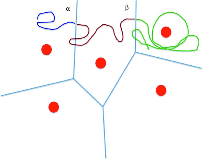
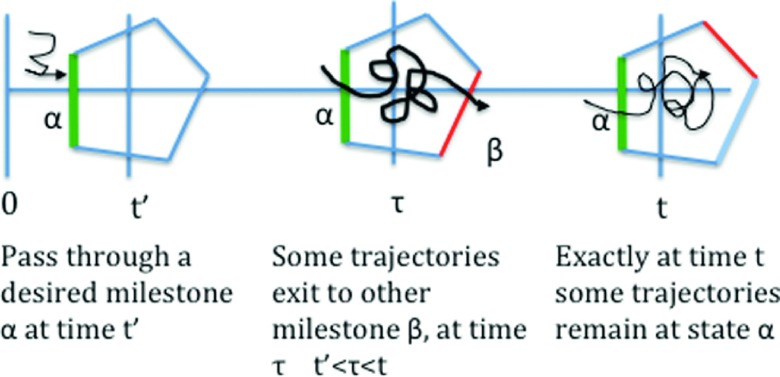
The sequence of events of Eq. (1) is illustrated schematically in Figures 1 and 2.

FIG. 1.

A schematic drawing of Milestoning in two dimensions. The milestones are the blue lines between the anchors (red circles). A trajectory is shown as a curve that alternates colors when the last milestone crossed is modified. In the illustration, it crossed milestone α and then β. See text for more details.

FIG. 2.

A schematic representation of the sequence of events considered in the basic Milestoning equation (Eq. (1)). The first event is the passage through milestone α at time t′. Then during propagation from time t‘ to t, some trajectories change their state by passing another milestone β. We consider only the fraction of trajectories that do not pass any other milestone up to time t as in state α.

While $q_{\alpha }\left(x,t\right)$ seems like a flux function in the sense of continuum mechanics, it is not the direct derivative of $p_{\alpha }\left(x,t\right)$. The time derivative of the probability of being at state α is

$${\displaystyle \frac{d{p}_{\alpha }\left(x,t\right)}{dt}=q_{\alpha }\left(x,t\right)-\sum _{\beta }\underset{M_{\beta }}{\int }\underset{0}{\overset{t}{\int }}{q}_{\alpha }\left(x,t^{\prime }\right)K_{\alpha \beta }\left(x,t^{\prime };x^{\prime },t\right)d{t}^{\prime }\cdot d{x}^{\prime }.}$$ (2)

Equation (2) is a sum of a gain and a loss at time t. We gain from trajectories that cross milestone α exactly at time t and lose trajectories that cross α (enter state α) earlier and exactly at t leave state α through another milestone β. The loss term is an integral over earlier entry times and summation over all exit channels β and x′.

Note that Eq. (1) is not closed. We expressed $p_{\alpha }\left(x,t\right)$ in terms of two other functions which at present are not known ($q_{\alpha }\left(x,t\right)$ and $K_{\alpha \beta }\left(x,t^{\prime };x^{\prime },t\right)$). We therefore write another equation for the flux. In our kinetic model, no particles are lost during a transition. Hence, we write an equation stating the conservation of trajectories in terms of the flux function,

$${\displaystyle q_{\alpha }\left(x,t\right)\cdot dt=\left\{\begin{array}{cc}\hfill p_{\alpha }\left(x,t=0\right)\cdot dt\hfill & \hfill t=0\hfill \\ \hfill \left[\sum _{\beta }\underset{0}{\overset{t}{\int }}\underset{M_{\beta }}{\int }{q}_{\beta }\left(x^{\prime },t^{\prime }\right)K_{\beta \alpha }\left(x^{\prime },t^{\prime };x,t\right)\cdot d{x}^{\prime }\cdot d{t}^{\prime }\right]\cdot dt\hfill & \hfill t>0\hfill \\ \hfill \hfill \end{array}\right\}.}$$ (3)

Equation (3) is at the center of the Milestoning theory and has the following physical meaning: we ask on the left side what is the probability that milestone α was crossed between time t and time t + dt at phase space point x. On the right hand side we count the pathways in which this transition may happen. If we are at time zero, then there is an initial condition (top term) that counts the trajectories that cross milestone α exactly at time 0. The lower term is for times that are different from zero. Crossing α at time t is by a trajectory of a well-defined state. Hence at earlier time, it must have crossed another milestone $\left(\beta \right)$. The summation and integral in Eq. (3) is over all the trajectories that cross milestone β at earlier times t′ and then continue to cross α exactly at time t. This summation accounts for all the events of crossing of α at time t. No other events in Ω that contribute to this transition are possible.

We will now show that Eq. (3) for the flux function $q_{\alpha }\left(x,t\right)$ can be solved exactly. The flux function is a core entity of Milestoning that enables the calculations of equilibrium and kinetic observables such as the free energy and the moments of the mean first passage time. It is therefore no wonder that we spent considerable time on the theory of how to compute $q_{\alpha }\left(x,t\right)$ and on an algorithm to extract it from MD trajectories.

C. An equation for the stationary flux function, q_α,stat(x)

To simplify the basic expression provided by Eq. (3), we consider stationary processes and stationary flux. A subset of stationary processes includes systems at equilibrium. We comment that even at equilibrium the flux is not necessarily zero. In the directional Milestoning picture proposed by Májek and Elber,¹⁶ the flux from cell i to cell j is considered a different function from the flux from cell j to i and it is not zero for a system at equilibrium at a finite temperature.

We consider processes for which a stationary long time limit is well defined. Of course, it is not guaranteed that a stationary solution exists and one can imagine a non-equilibrium process with an oscillating external force for which the flux never becomes stationary. However, in the current formulation, we restrict ourselves to stationary, long-time processes. The goal of the current section is the derivation of an equation for the stationary flux $q_{\alpha ,\mathit{stat}}\left(x\right)$.

Another restriction is the type of processes that we consider which is of processes homogeneous in time. For example, typical MD trajectories with time independent potentials are time homogeneous. In this case, the kernel does not depend on the absolute times but only on the time difference; hence, we write

$${\displaystyle K_{\beta \alpha }\left(x^{\prime },t^{\prime };x,t\right)\to K_{\beta \alpha }\left(x^{\prime };x,t-t^{\prime }\right).}$$

The Laplace transform is a convenient approach to handle Eqs. (1) and (3) because both equations are convolutions of time homogeneous processes. After the Laplace transform, the convolutions are reduced to algebraic products, which are simpler to manipulate. Moreover, it is easy to use Laplace transformed functions to derive the long time limit as we illustrate below.

We express the stationary flux in terms of the Laplace transform of the time dependent flux function. We define the Laplace transform of a function $g\left(t\right)$ as $\tilde{g}\left(u\right)=\underset{0^{-}}{\overset{\infty }{\int }}exp\left(-ut\right)g\left(t\right)dt$, where u is the Laplace variable, and the time integral starts from small negative values. For the flux function, we write

$${\displaystyle {\tilde{q}}_{\alpha }\left(x,u\right)=\underset{0^{-}}{\overset{\infty }{\int }}{q}_{\alpha }\left(x,t\right)exp\left(-ut\right)dt.}$$ (4)

Consider now a time $\overline{t}$ that is finite but sufficiently long such that for all practical purposes, the flux $q_{\alpha }\left(x,\overline{t}\right)$ is time independent (stationary) and is equal to $q_{\alpha ,\mathit{stat}}\left(x\right)$. We can separate Eq. (4) to two integrals

$${\displaystyle {\tilde{q}}_{\alpha }\left(x,u\right)=\underset{0^{-}}{\overset{\overline{t}}{\int }}{q}_{\alpha }\left(x,t\right)exp\left(-ut\right)dt+\underset{\overline{t}}{\overset{\infty }{\int }}{q}_{\alpha ,\mathit{stat}}\left(x\right)exp\left(-ut\right)dt=\underset{0^{-}}{\overset{\overline{t}}{\int }}{q}_{\alpha }\left(x,t\right)exp\left(-ut\right)dt+q_{\alpha ,\mathit{stat}}\left(x\right)\cdot \frac{1}{u}exp\left(-u\overline{t}\right).}$$

Multiplying the above equation by the Laplace variable u and taking the limit of u → 0, we have

$${\displaystyle \begin{array}{rcl}\hfill \underset{u\to 0}{lim}\left[u\cdot {\tilde{q}}_{\alpha }\left(x,u\right)\right]& \hfill =\hfill & \underset{u\to 0}{lim}\left[u\cdot \underset{0^{-}}{\overset{\overline{t}}{\int }}{q}_{\alpha }\left(x,t\right)exp\left(-ut\right)dt\right]\hfill \\ \hfill & \hfill \hfill & +\underset{u\to 0}{lim}\left[u\cdot q_{\alpha ,\mathit{stat}}\left(x\right)\cdot \frac{1}{u}exp\left(-u\overline{t}\right)\right],\hfill \\ \hfill \underset{u\to 0}{lim}\left[u\cdot {\tilde{q}}_{\alpha }\left(x,u\right)\right]& \hfill =\hfill & q_{\alpha ,\mathit{stat}}\left(x\right).\hfill \end{array}}$$ (5)

Similarly, we define the Laplace transform of the time homogeneous kernel

$${\displaystyle {\tilde{K}}_{\beta \alpha }\left(x^{\prime };x,u\right)=\underset{0^{-}}{\overset{\infty }{\int }}{K}_{\beta \alpha }\left(x^{\prime };x,\tau \right)exp\left(-u\tau \right)d\tau .}$$ (6)

Consider the Laplace transform of the kernel at the limit of u → 0,

$${\displaystyle \underset{u\to 0}{lim}\left[{\tilde{K}}_{\beta \alpha }\left(x^{\prime };x,u\right)\right]=\underset{u\to 0}{lim}\left[\underset{0^{-}}{\overset{\infty }{\int }}{K}_{\beta \alpha }\left(x^{\prime };x,\tau \right)exp\left(-u\tau \right)d\tau \right]=\underset{0^{-}}{\overset{\infty }{\int }}{K}_{\beta \alpha }\left(x^{\prime };x,\tau \right)d\tau ,}$$ (7)

$${\displaystyle \underset{u\to 0}{lim}\left[{\tilde{K}}_{\beta \alpha }\left(x^{\prime };x,u\right)\right]\equiv K_{\beta \alpha }\left(x^{\prime };x\right),}$$

Equation (7) has a simple physical interpretation as the probability that a trajectory will cross milestone α at phase space point x for the first time given that it crossed milestone β at phase space point x′ before. The actual time difference between the crossings no longer matters. For future reference, we also define the time independent kernel—$K_{\beta \alpha }\left(x^{\prime };x\right)$.

Keeping Eq. (5) in mind, we now take the Laplace transform of Eq. (3), multiply the result by the Laplace variable u, and take the limit of u → 0,

$${\displaystyle \underset{u\to 0}{lim}\left[u\cdot {\tilde{q}}_{\alpha }\left(x,u\right)\right]=\underset{u\to 0}{lim}\left[u\cdot p_{\alpha }\left(x,t=0\right)\right]+\underset{u\to 0}{lim}\left[\sum _{\beta }\underset{M_{\beta }}{\int }d{x}^{\prime }\cdot u\cdot {\tilde{q}}_{\beta }\left(x^{\prime },u\right){\tilde{K}}_{\beta \alpha }\left(x^{\prime };x,u\right)\right].}$$ (8)

The first term on the right hand side of Eq. (8) vanishes, as it should for initial conditions that have no impact on the stationary solution. We use Eqs. (5) and (7) to write

$${\displaystyle q_{\alpha ,\mathit{stat}}\left(x\right)=\sum _{\beta }\underset{M_{\beta }}{\int }d{x}^{\prime }{q}_{\beta ,\mathit{stat}}\left(x^{\prime }\right)\cdot K_{\beta \alpha }\left(x^{\prime };x\right).}$$ (9)

Equation (9) is a linear equation for the vector q_stat with the milestone number as an index. The kernel is known exactly from short MD trajectories between milestones. Given a set of initial conditions at the interface (provided as a sample from the flux function), the kernel transformed these initial conditions by trajectory calculations into hitting points on nearby milestones. We can write Eq. (9) more compactly using bold-faced letters to denote vectors and matrices. We have

$${\displaystyle {{\mathbf{q}}^t}_{\mathit{stat}}={{\mathbf{q}}^t}_{\mathit{stat}}\mathbf{K}.}$$ (10)

Both the vector and the matrix are typically of high dimension. However, the kernel is known exactly and is a transition probability. This facilitates the computational algorithm, which is described next.

D. An algorithm to compute the stationary flux

Equation (10) is a linear problem on the unknown q^t given the transition kernel (matrix) K. The linear problem can be solved, in principle, by standard means. For example, the left eigenvector of the matrix K with an eigenvalue of one is the desired solution for Eq. (10). All the absolute values of the eigenvalues of K are between zero and one and the eigenvector with eigenvalue one is unique if the system is ergodic. This also follows from the kernel being a transition matrix. It is therefore clear that multiplying q^t by K numerous times will reduce the contributions of all the eigenvalues that are smaller than one and will retain the desired solution.³¹

We solve for the flux vector q^t Eq. (10) by power iterations.³¹ The iterations are over flux vectors and are denoted by ${\left\{{\mathbf{q}}^{\left(n\right)t}\right\}}_{n=0}^N$, where N is the number of iterations used. The sequence of iterations is given by

$${\displaystyle \left\{\begin{array}{cc}\hfill q_{\alpha }^{\left(0\right)}\left(x\right)\propto exp\left(-\beta H\left(x\right)\right)\hfill & \hfill x\in M_{\alpha }\forall \alpha \hfill \\ \hfill {\mathbf{q}}^{\left(n+1\right)t}={\mathbf{q}}^{\left(n\right)t}\mathbf{K}\hfill & \hfill n=0,1,2,\dots .\hfill \end{array}\right.}$$ (11)

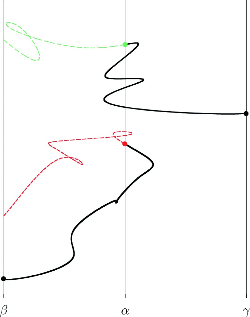
The Boltzmann distribution follows from the NVT ensemble and is clearly not exactly the flux, hence the need for iterations. We generate a sample from the Boltzmann distribution by Monte Carlo (MC) or MD algorithms tailored for constant temperature simulations conditioned to be at milestone α. A better initial guess can be obtained by computing forward and backward trajectories to the nearby interfaces. The phase space points, provided by the exact flux function, are sampled from a first hitting distribution. That is, integration backward in time of the phase space points yields trajectories that cross first a milestone different from the starting milestone (Figure 3). This picture was discussed first in the context of PPTIS.⁷ We implemented this condition for acceptance of trajectories in directional Milestoning¹⁶ to increase the accuracy of the initial flux function avoiding the over counting of trajectories that cross the same interface multiple times. Each trajectory must be counted only once regardless of the number of times it crosses sequentially and repeatedly the same interface. Hawk and Makarov introduced a filter that extends to more than one milestone.³²

FIG. 3.

A schematic drawing of trajectory fragments initiated at milestone α. Backward trajectories in time (dashed lines) are used to assess if the trajectories are sampled from FHPD. The red dashed trajectory re-crosses the initial milestone α before hitting milestone β. Therefore, it is not sampled from FHPD. The green trajectory hits milestone β before any other milestone and is sampled from FHPD. Note that the forward trajectories (black lines) are allowed to re-cross the initial milestone before they finally terminate at a nearby milestone. The forward trajectories illustrate the operation of the transition matrix K that takes phase space points from one milestone and transmits them with certain probability to phase space points at another milestone. For Milestoning calculations, we also record the time length of the forward trajectory fragments (black lines). It is possible to exploit the identity of the terminating milestones of the backward trajectories (dashed lines) as well, but so far we have not done so. The final termination points of the trajectories (for example, the black circle at milestone β) are used as starting points for the next iteration of the flux ${\mathbf{q}}^{\left(n+1\right)}$.

Even this filter is not providing the exact flux function since we have no record of the fate of the trajectories beyond the nearby interfaces. It is possible that the distribution at a nearby interface is still inaccurate. The condition provided in Eq. (11) is global and it cannot be satisfied exactly by local considerations unless iterations are applied. In principle, the initial guess for the flux function should not affect the final results, however, the number of iterations that is required to obtain the correct answer is influenced by the initial condition. It makes sense to try to determine a best approximation to the flux function locally and to reduce the number of required (expensive) iterations.

The iterations have a simple physical interpretation. We initiate trajectories at a milestone and continue these trajectories to the nearby milestones. The next iteration uses the final phase space point of the previous terminating trajectories at a milestone as initial conditions and continues these trajectories to yet another layer of milestones. Hence, each of the iterations extends the time length of the trajectories. If a very large number of iterations are used, exact long trajectories are generated. Hence, it is not surprising that Milestoning becomes exact at the limit of a large number of power iterations. Of course, this particular scenario suggests no computational advantage compared to straightforward molecular dynamics. It only suggests a formal connection to exact calculations and an analysis method.²⁹ We expect, as we illustrate a number of times in the past, that if the system is close to equilibrium, rapid convergence to the correct flux can be achieved using good guesses (and only short trajectories).

The flux is not normalized in the usual sense. For convenience, we write

$${\displaystyle q_{\alpha ,\mathit{stat}}\left(x\right)=w_{\alpha }{f}_{\alpha }\left(x\right),}$$ (12)

where w_α is an undetermined weight that defines the relative contributions of different milestones to the overall flux. This weight is a prime target of the computations since it is useful in various numerical variants of Milestoning. For example, w_α determines the weights of edges for molecular kinetic networks.³³ It is the only term that carries information about the kinetics in the zero iteration, since the distribution within the milestone $\left(f_{\alpha }^{\left(0\right)}\left(x\right)\right)$ is of equilibrium. Hence, a physical interpretation of the zero iteration is of a system that is equilibrated within a milestone but not necessarily between milestones. The local equilibrium within a milestone is the “memory loss” approximation that was used in the first version of Milestoning.³⁴ It is assumed that trajectories spend enough time between the milestones such that the distribution on the terminating milestone is of local equilibrium. This separation of time scales can be achieved by proper selection of the interfaces. For example, if a picture of a single reaction coordinate is appropriate and if the space normal to the reaction coordinate is small and local equilibrium in the milestone can be achieved rapidly, then the memory loss assumption is likely to be valid.¹⁴ In a reduced coarse-grained description of the system, only the milestones and their weights remain.

We emphasize that the above considerations of “memory loss” are not required in exact Milestoning. In exact Milestoning, the iterations guarantee convergence to the exact answer regardless of the initial guess for the flux function. Poor initial guesses may cause however slower convergence rate.

The function $f_{\alpha }\left(x\right)$ is normalized,

$${\displaystyle \int f_{\alpha }\left(x\right)dx=1.}$$ (13)

Note that the Eq. (10) determines the overall flux only up to a multiplying constant, λ, which we take to be positive. Hence, if ${\left(q_{\alpha ,\mathit{stat}}\left(x\right)=w_{\alpha }{f}_{\alpha }\left(x\right)\right)}_{\alpha =1}^M$ is a solution of Eq. (10), so is the vector ${\left(\lambda \cdot w_{\alpha }{f}_{\alpha }\left(x\right)\right)}_{\alpha =1}^M$.

The second line of Eq. (11) requires the calculations of a high dimensional integral over the phase space points x. Each phase space point is used to initiate a trajectory fragment that runs to termination, which is formally equivalent to the operation of K on the initial phase space point. We calculate this integral by sampling in phase space. The sampling is conducted according to the flux ${\mathbf{q}}^{\left(n\right)}$. In the first iteration, the sample is determined by the canonical distribution. In the next iteration, we use points that were created by terminating trajectories at the milestones. Let the set of nth iteration phase space points at milestone α be ${\left\{x_{\alpha i}^{\left(n\right)}\right\}}_{i=1}^{L_{\alpha }}$, where L_α is the number of sampled points. The probability density associated with this set is

$${\displaystyle q_{\alpha ,\mathit{stat}}^{\left(n\right)}\left(x\right)=\frac{w_{\alpha }^{\left(n\right)}}{L_{\alpha }}\sum _{i=1,\dots \underset{\alpha }{L}}\delta \left(x-x_{\alpha i}^{\left(n\right)}\right)}$$ (14)

which is equivalent to approximating the function $f_{\alpha }\left(x\right)$ in Eq. (12) by a sum of Dirac’s delta functions. Operating on this set yields a new set of phase space points using Eq. (11),

$${\displaystyle \frac{w_{\alpha }^{\left(n+1\right)}}{L_{\alpha }}\sum _{i=1,\dots \underset{\alpha }{L}}\delta \left(x-x_{\alpha i}^{\left(n+1\right)}\right)=\sum _{\beta }\frac{w_{\beta }^{\left(n\right)}}{L_{\beta }}\int \sum _{j=1,\dots \underset{\beta }{L}}\delta \left(x^{\prime }-x_{\beta j}^{\left(n\right)}\right){\mathbf{K}}_{\beta \alpha }\left(x^{\prime },x\right)d{x}^{\prime },}$$ (15)

$${\displaystyle w_{\alpha }^{\left(n+1\right)}=\sum _{\beta }{w}_{\beta }^{\left(n\right)}\left[\sum _{i=1,\dots ,\underset{\alpha }{L}}\sum _{j=1,\dots \underset{\beta }{L}}{\mathbf{K}}_{\beta \alpha }\left(x_{\beta j}^{\left(n\right)},x_{\alpha i}^{\left(n+1\right)}\right)/\left(L_{\alpha }{L}_{\beta }\right)\right].}$$

The second line is obtained by integration of the phase space variable x in the first line of Eq. (15). The final formula is a direct equation for the vector of weights of the milestones w. At the limit of sufficient number of iterations, we have ${\mathbf{w}}^{\left(n+1\right)}\to {\mathbf{w}}^{\left(n\right)}$. It is convenient to re-write Eq. (15) as a linear equation for the vector of coefficients ${\mathbf{w}}^{\left(n+1\right)}$, which is consistent with the approximate variation of Milestoning.¹² Equation (15) is a power iteration of the type ${\mathbf{w}}^{\left(n+1\right)t}={\mathbf{w}}^{\left(n\right)t}\mathbf{K}$ and it converges to the dominant eigenvector of the matrix K. It can also be cast as an eigenvector problem and, as such, one can use an eigenvalue solver with better convergence. Both equations converge to the same limit,

$${\displaystyle \frac{w_{\alpha }^{\left(n+1\right)}}{L_{\alpha }}\sum _{i=1,\dots \underset{\alpha }{L}}\delta \left(x-x_{\alpha i}^{\left(n+1\right)}\right)=\sum _{\beta }\frac{w_{\beta }^{\left(n+1\right)}}{L_{\beta }}\int \sum _{j=1,\dots \underset{\beta }{L}}\delta \left(x^{\prime }-x_{\beta j}^{\left(n\right)}\right){\mathbf{K}}_{\beta \alpha }\left(x^{\prime },x\right)d{x}^{\prime },}$$ (16)

$${\displaystyle w_{\alpha }^{\left(n+1\right)}=\sum _{\beta }{w}_{\beta }^{\left(n+1\right)}\left[\sum _{i=1,\dots ,\underset{\alpha }{L}}\sum _{j=1,\dots \underset{\beta }{L}}{\mathbf{K}}_{\beta \alpha }\left(x_{\beta j}^{\left(n\right)},x_{\alpha i}^{\left(n+1\right)}\right)/\left(L_{\alpha }{L}_{\beta }\right)\right].}$$

In practical applications, the length of the vector and the dimensionality of the transition matrix, once the phase space variables are integrated out, are manageable and so far have not exceeded tens of thousands. With the weight of the milestones calculated, the fluxes in Eq. (14) can be determined as well.

An important question is the error assessment and tests of the convergence of the iterations. In general, we use ensemble averages to test convergence. This is because we can estimate them with reasonable accuracy even for large systems. For example, we may consider $w_{\alpha }\equiv \underset{M_{\alpha }}{\int }{q}_{\alpha }\left(x_{\alpha }\right)d{x}_{\alpha }$. However, for the small and simple test case, we consider here it is possible to look at the results at greater details. We therefore introduce also the Rayleigh quotient r for the fluxes which is given by

$${\displaystyle r\equiv \frac{〈{\mathbf{q}}^{\left(n+1\right)},{\mathbf{q}}^{\left(n\right)}〉}{〈{\mathbf{q}}^{\left(n\right)},{\mathbf{q}}^{\left(n\right)}〉}=\frac{〈{\mathbf{q}}^{\left(n\right)}\mathbf{K},{\mathbf{q}}^{\left(n\right)}〉}{〈{\mathbf{q}}^{\left(n\right)},{\mathbf{q}}^{\left(n\right)}〉},}$$ (17)

where the $〈\cdot ,\cdot 〉$ is the L₂ inner product. The Rayleigh quotient is bound between minus one and one since the kernel K does not increase the length of a vector. It is equal to one if the results are converged. Our representation of the flux density uses Dirac delta functions.

The second convergence measure that we used is the relative error in the 1-norm, Δ, between flux vectors of sequential iterations,

$${\displaystyle {\mathrm{\Delta }}_{\alpha }={‖q_{\alpha }^{\left(n-1\right)}-q_{\alpha }^{\left(n\right)}‖}_1/{‖q_{\alpha }^{\left(n\right)}‖}_1.}$$ (18)

The simulations converge when Δ_α = 0. These measures are useful also for conducting the iterations optimally. It is possible that fluxes at selected milestones vary slowly or converge rapidly. Therefore an adaptive iterative scheme is possible and likely to show efficiency gains. We illustrate this phenomenon in Sec. III.

We summarize below the algorithm for computing the stationary flux q.

1. For each milestone M_α, sample configurations, x_α, from a known trial distribution, typically canonical $q_{\alpha }\left(x\right)\propto exp\left(-H\left(x\right)/kT\right)x\in M_{\alpha }$.

2. Compute forward trajectories from the points x_α sampled from the current q_α for all α. We record the initial and final points of the trajectory fragments as well as the time length. This operation samples the matrix product q^t ⋅ K. The time length of the trajectories is used in other calculations.

3. Estimate the total flux through the interface α by summing up the points that terminate at α. This operation is equivalent to the integration $w_{\alpha }^{\left(n+1\right)}=\underset{M_{\alpha }}{\int }{q}_{\alpha }^{\left(n+1\right)}\left(x_{\alpha }\right)d{x}_{\alpha }$.

4. Check convergence of the iterations: (1) $|〈\mathbf{qK},\mathbf{q}〉/〈\mathbf{q},\mathbf{q}〉-1|<\epsilon$, (2) ${‖q_{\alpha }^{\left(n-1\right)}-q_{\alpha }^{\left(n\right)}‖}_1/{‖q_{\alpha }^{\left(n\right)}‖}_1\le \epsilon$, or by (3) observables of interest. If the calculation has not converged, use the final phase space points of the trajectory fragment to obtain a new q_α and go to 2.

The stationary flux function is the basic entity of the Milestoning theory and algorithm. However, it is not a common experimental observable. To make the connection to the more typical observables of equilibrium and kinetics, we show below how (with the help of the flux function) we can determine the probability of a state and its free energy (Sec. II E). We follow up with the calculations of the moments of the first passage time (Sec. II F).

We finally comment that the original version of Milestoning⁹ is a simplified form of the exact Milestoning formulation. In the original version, no iterations were conducted and the trial distribution $q_{\alpha }\left(x\right)\propto exp\left(-H\left(x\right)/kT\right)x\in M_{\alpha }$ was used in the equation for the weights of the milestones (Eq. (15)). There was no further refinement of the distribution within the milestone. Hence, the memory loss approximation was used.

E. The stationary probability

We consider the probability, $p_{\alpha }\left(x,t\right)$, that M_α is the last milestone that was passed at a phase space point x before time t. At stationary or equilibrium conditions, the dependence on time can be omitted and we use this probability to define a corresponding “free energy” as $F_{\alpha }\left(x\right)=-\left(k_{B}T\right)\cdot log\left(p_{\alpha }\left(x\right)\right)$, where the temperature, T, and the Boltzmann constant, k_B, enters the calculations through the initial conditions of the trajectories (see Sec. II D and Eq. (11)). As we have done for the flux, we consider the Laplace transform for the probability (Eq. (1)) to have

$${\displaystyle {\tilde{p}}_{\alpha }\left(x,u\right)={\tilde{q}}_{\alpha }\left(x,u\right)\cdot \frac{1}{u}\left[1-\sum _{\beta }\underset{M_{\beta }}{\int }d{x}^{\prime }{\tilde{K}}_{\alpha \beta }\left(x,x^{\prime },u\right)\right].}$$ (19)

We multiply Eq. (21) by the Laplace variable u and consider the limit in which it is approaching zero. This is the long time limit that gives the stationary solution of the probability (similar to the limit of the flux function in Eq. (5)),

$${\displaystyle \underset{u\to 0}{lim}u\cdot {\tilde{p}}_{\alpha }\left(x,u\right)=p_{\alpha ,\mathit{stat}}\left(x\right).}$$ (20)

We elaborate on the expression on the right hand side of Eq. (19),

$${\displaystyle \underset{u\to 0}{lim}\frac{1}{u}\left[1-\sum _{\beta }\underset{M_{\beta }}{\int }d{x}^{\prime }{\tilde{K}}_{\alpha \beta }\left(x,x^{\prime },u\right)\right]=\underset{u\to 0}{lim}\frac{1}{u}\left[1-\sum _{\beta }\underset{0^{-}}{\overset{\infty }{\int }}\underset{M_{\beta }}{\int }dt\cdot d{x}^{\prime }\cdot exp(-ut)K_{\alpha \beta }\left(x,x^{\prime },t\right)\right]=\underset{u\to 0}{lim}\frac{1}{u}\left[1-\sum _{\beta }\underset{0^{-}}{\overset{\infty }{\int }}\underset{M_{\beta }}{\int }dt\cdot d{x}^{\prime }\cdot \left\{1-ut\right\}{K}_{\alpha \beta }\left(x,x^{\prime },t\right)\right]=\underset{u\to 0}{lim}\frac{1}{u}\left[1-\sum _{\beta }\underset{0^{-}}{\overset{\infty }{\int }}dt\underset{M_{\beta }}{\int }d{x}^{\prime }{K}_{\alpha \beta }\left(x,x^{\prime },t\right)\right.+\left.u\sum _{\beta }\underset{0^{-}}{\overset{\infty }{\int }}dt\underset{M_{\beta }}{\int }d{x}^{\prime }\cdot t\cdot K_{\alpha \beta }\left(x,x^{\prime },t\right)\right]=\underset{u\to 0}{lim}\frac{1}{u}\left[1-1+u\sum _{\beta }\underset{0^{-}}{\overset{\infty }{\int }}dt\underset{M_{\beta }}{\int }d{x}^{\prime }\cdot t\cdot K_{\alpha \beta }\left(x,x^{\prime },t\right)\right]=\sum _{\beta }\underset{0^{-}}{\overset{\infty }{\int }}dt\underset{M_{\beta }}{\int }d{x}^{\prime }\cdot t\cdot K_{\alpha \beta }\left(x,x^{\prime },t\right)\equiv 〈t_{\alpha }\left(x\right)〉,}$$ (21)

where we denote the average lifetime of a position x_α at milestone α as $〈t_{\alpha }\left(x\right)〉$. It is the average time that it takes a trajectory initiated at x_α to reach a milestone different from α for the first time. We now combine Eqs. (19) to (21) to obtain

$${\displaystyle \underset{u\to 0}{lim}\left[{\tilde{p}}_{\alpha }\left(x,u\right)\right]=\underset{u\to 0}{lim}\left[{\tilde{q}}_{\alpha }\left(x,u\right)\cdot \frac{1}{u}\left[1-\sum _{\beta }\underset{M_{\beta }}{\int }d{x}^{\prime }{\tilde{K}}_{\alpha \beta }\left(x,x^{\prime },u\right)\right]\right],}$$ (22)

$${\displaystyle p_{\alpha ,\mathit{stat}}\left(x\right)=q_{\alpha ,\mathit{stat}}\left(x\right)\cdot 〈t_{\alpha }\left(x\right)〉.}$$

The last expression is a remarkably simple result for the probability of being at state α. It is a product of the stationary flux function to cross milestone α multiplied by the average time that the crossing trajectory lives in this state (before crossing another milestone). We call this time—the lifetime of a milestone. Compared to the previous calculations of the flux function, we need to add only a single new entity (the milestone lifetime) that can be computed from the same trajectory fragments that we used to estimate the flux. If we sample L_α trajectories at milestone α and phase space point x with termination times at other milestones ${\left\{t_i\right\}}_{i=1}^{L_{\alpha }}$, the lifetime of milestone α at phase space point x is $〈t_{\alpha }\left(x\right)〉=\frac{1}{L_{\alpha }}\sum _{i=1,\dots ,L_{\alpha }}{t}_i$. Hence, no new trajectories are required.

F. The mean first passage time

To study kinetics, we focus on the first passage time. The first passage time is defined as the time it takes the system to reach for the first time a state f given that it started from a state i. The first passage time is a random variable that can be sampled with trajectory calculations or its distribution function can be computed. We prefer to calculate the moments of the distribution function of the first passage time. In particular, the first moment of this distribution, $〈\tau 〉$, or the MFPT is widely used to study kinetics. For reactants’ population that decays exponentially in time, the MFPT is the inverse of the rate constant.

To model the first arrival to the final state, we consider a specific choice of the kernel with an absorbing boundary at milestone f which we call K_A. We set

$${\displaystyle K_{A,f\alpha }\left(x;x^{\prime },t\right)=0\forall \alpha .}$$ (23)

The MFPT or $〈\tau 〉$ is the time that it takes a trajectory to enter the absorbing state multiplied by the probability to enter the absorbing state at time t, averaged over all times. In other words, it is the first moment in time of the flux at milestone f,

$${\displaystyle 〈\tau \left(x\right)〉=\underset{0^{-}}{\overset{\infty }{\int }}t\cdot q_f\left(x,t\right)dt\text{ or }〈{\tau }_f〉=\underset{M_f}{\int }d{x}_f\underset{0^{-}}{\overset{\infty }{\int }}dt\cdot t\cdot q_f\left(x,t\right).}$$ (24)

It is important to note that the flux as defined in Eq. (24) is no longer stationary. This is a result of the choice of the kernel made in Eq. (23). The kernel is no longer conserving and the flux is decaying as a function of time. This is necessary since Eq. (24) is diverging for a non-zero stationary flux.

We can write the integral over time as a derivative in Laplace space,

$${\displaystyle \underset{0^{-}}{\overset{\infty }{\int }}t\cdot q_f\left(x,t\right)dt=\underset{u\to 0}{lim}\underset{0^{-}}{\overset{\infty }{\int }}exp\left(-ut\right)t\cdot q_f\left(x,t\right)dt=-\underset{u\to 0}{lim}\frac{d}{du}\underset{0^{-}}{\overset{\infty }{\int }}exp\left(-ut\right)q_f\left(x,t\right)dt=-\underset{u\to 0}{lim}\frac{d}{du}{\tilde{q}}_f\left(x,u\right).}$$ (25)

We already discussed ${\tilde{q}}_{\alpha }\left(x_{\alpha },u\right)$ (see, for instance, Eq. (8)) which we could further exploit for our purpose here,

$${\displaystyle \begin{array}{rcl}\hfill {\tilde{q}}_{\alpha }\left(x,u\right)& \hfill =\hfill & p_{\alpha }\left(x,t=0\right)\hfill \\ \hfill & \hfill \hfill & +\sum _{\beta }\underset{M_{\beta }}{\int }d{x}^{\prime }\cdot {\tilde{q}}_{\beta }\left(x^{\prime },u\right){\tilde{K}}_{A,\beta \alpha }\left(x^{\prime },x_{\alpha },u\right),\hfill \\ \hfill \frac{d{\tilde{q}}_{\alpha }\left(x,u\right)}{du}& \hfill =\hfill & \sum _{\beta }\underset{M_{\beta }}{\int }d{x}^{\prime }\left[\frac{d{\tilde{q}}_{\beta }\left(x^{\prime },u\right)}{du}{\tilde{K}}_{A,\beta \alpha }\left(x^{\prime },x,u\right)\right.\hfill \\ \hfill & \hfill \hfill & +\left.{\tilde{q}}_{\beta }\left(x^{\prime },u\right)\frac{d{\tilde{K}}_{A,\beta \alpha }\left(x^{\prime },x,u\right)}{du}\right].\hfill \end{array}}$$ (26)

Or in a more compact matrix notation,

$${\displaystyle \begin{array}{c}\hfill {\tilde{\mathbf{q}}}^t\left(\mathbf{I}-{\tilde{\mathbf{K}}}_A\right)={\mathbf{p}}^t\left(t=0\right),\hfill \\ \hfill {\frac{d\tilde{\mathbf{q}}}{du}}^t\left(\mathbf{I}-{\tilde{\mathbf{K}}}_A\right)-{\tilde{\mathbf{q}}}^t\frac{d}{du}{\tilde{\mathbf{K}}}_A=0.\hfill \end{array}}$$ (27)

We determine the derivative of $\tilde{\mathbf{q}}$ with respect to the Laplace variable in the compact notation

$${\displaystyle \frac{d{\tilde{\mathbf{q}}}^t}{du}={\tilde{\mathbf{q}}}^t\frac{d{\tilde{\mathbf{K}}}_A}{du}{\left(\mathbf{I}-{\tilde{\mathbf{K}}}_A\right)}^{-1}={\mathbf{p}}^t\left(t=0\right)\cdot {\left(\mathbf{I}-{\tilde{\mathbf{K}}}_A\right)}^{-1}\frac{d{\tilde{\mathbf{K}}}_A}{du}{\left(\mathbf{I}-{\tilde{\mathbf{K}}}_A\right)}^{-1}.}$$ (28)

We define the matrix ${\mathbf{K}}_A\equiv \underset{u\to 0}{lim}{\tilde{\mathbf{K}}}_A=\underset{0^{-}}{\overset{\infty }{\int }}{\mathbf{K}}_A\left(t\right)dt$. Hence, whenever we do not write explicit time dependence, we imply integration over time.

We also consider the matrix of local average transition times between the milestones, T. This matrix is also minus the derivative of the Laplace transform of the matrix ${\tilde{\mathbf{K}}}_A\left(u\right)$ at the limit of zero Laplace variables. It has a simple physical interpretation. It is the first moment of time of the probability transition matrix ${\mathbf{K}}_A\left(t\right)$,

$${\displaystyle \mathbf{T}=-\underset{u\to 0}{lim}\frac{d{\tilde{\mathbf{K}}}_A\left(u\right)}{du}=-\underset{u\to 0}{lim}\frac{d}{du}\left[\underset{0^{-}}{\overset{\infty }{\int }}exp\left(-ut\right)\cdot {\mathbf{K}}_A\left(t\right)dt\right]=\underset{0^{-}}{\overset{\infty }{\int }}t\cdot {\mathbf{K}}_A\left(t\right)dt.}$$ (29)

Note that $〈\tau 〉=-\underset{u\to 0}{lim}\frac{d{\tilde{q}}_f}{du}$ so the negative signs of T and $〈\tau 〉$ that emerge from the differentiation with respect to the Laplace variable cancel out to give

$${\displaystyle {〈\overrightarrow{\tau }〉}^t={\mathbf{p}}^t\left(t=0\right)\cdot {\left(\mathbf{I}-{\mathbf{K}}_A\right)}^{-1}\mathbf{T}{\left(\mathbf{I}-{\mathbf{K}}_A\right)}^{-1}.}$$ (30)

We note that the transition time is a function of the phase space points at the two interfaces. Interestingly, the explicit dependence on the absorbing milestone disappears in the final expression as is illustrated by further manipulations below. This is typical to Markovian processes in which the MFPT depends only on the starting and not the end point.⁹

The MFPT in Eq. (30) is a vector that contains information on all milestones. Here, we are interested only in the average time to reach for the first time the absorbing milestone f. Hence, we are interested in a single element of the vector ${\left({〈\overrightarrow{\tau }〉}^t\right)}_f$. To obtain this single element, we multiply Eq. (32) from the right by a column vector ${\mathbf{e}}_f\left(x_f\right)$ which is a unit vector in the direction of the absorbing milestone. The scalar product implies an integration over the phase space points of the absorbing milestone, x_f, to have

$${\displaystyle {〈\overrightarrow{\tau }〉}^t\cdot {\mathbf{e}}_f={\mathbf{p}}^t\left(t=0\right)\cdot {\left(\mathbf{I}-{\mathbf{K}}_A\right)}^{-1}\mathbf{T}{\left(\mathbf{I}-{\mathbf{K}}_A\right)}^{-1}\cdot {\mathbf{e}}_f.}$$ (31)

As stated in the definition the rows of the transition matrix K (including the integration over the phase space points in the milestone) must add to one. The matrix K_A is different since the elements of the row of the absorbing state in K_A, and obviously their sum, are zero. As a result, the matrix K_A has non-negative eigenvalues smaller than one. This implies that the inverse of $\left(\mathbf{I}-{\mathbf{K}}_A\right)$ in Eq. (31) is well defined. The summation of the rows of K_A can be written as

$${\displaystyle {\mathbf{K}}_A\cdot \mathbf{1}=\mathbf{1}-{\mathbf{e}}_f,}$$ (32)

where 1 is a column vector. Each of the elements of 1 is equal 1. Using Eq. (32), we can write

$${\displaystyle \left(\mathbf{I}-{\mathbf{K}}_A\right)\mathbf{1}={\mathbf{e}}_f,\mathbf{1}={\left(\mathbf{I}-{\mathbf{K}}_A\right)}^{-1}{\mathbf{e}}_f.}$$ (33)

Substituting in Eq. (31), we have

$${\displaystyle {〈\overrightarrow{\tau }〉}^t\cdot {\mathbf{e}}_f={\mathbf{p}}^t\left(t=0\right)\cdot {\left(\mathbf{I}-{\mathbf{K}}_A\right)}^{-1}\mathbf{T}\cdot \mathbf{1}.}$$ (34)

Consider the matrix vector product t ≡ T ⋅ 1. The resulting elements of the column vector t are the summation of the row of the matrix T. For example,

$${\displaystyle t_{\alpha }\left(x\right)=\sum _{\beta }\underset{M_{\beta }}{\int }{T}_{\alpha \beta }\left(x,x^{\prime }\right)d{x}^{\prime }=\sum _{\beta }\underset{0}{\overset{\infty }{\int }}\underset{M_{\beta }}{\int }dt\cdot d{x}^{\prime }\cdot t\cdot {K{}_{A,}}_{\alpha \beta }\left(x,x^{\prime },t\right).}$$ (35)

Equation (36) therefore takes its final compact form

$${\displaystyle {〈\overrightarrow{\tau }〉}_f={\mathbf{p}}^t\left(t=0\right)\cdot {\left(\mathbf{I}-{\mathbf{K}}_A\right)}^{-1}\mathbf{t}.}$$ (36)

Equation (36) is central to the understanding of kinetics as the MFPT plays an important role in many theories, experiments, and simulations of molecular processes. Interestingly, if the kernel is replaced by a single exponential function,⁹ $K_{\alpha \beta }\propto exp\left(-t/t_{\alpha }\right)$ which implies a Markov process,^34,37 we obtain the same expression as Eq. (36) where $t_{\alpha }={\left(\mathbf{t}\right)}_{\alpha }$.

The expression in Eq. (36) can be difficult to compute in exact Milestoning since the solution of a large linear system $\left(\mathbf{I}-{\mathbf{K}}_A\right)$ or a geometric series expansion in K_A is required. In the original version of Milestoning, this was of a smaller concern since the matrix depends only on the milestone index and not on the phase space point in the Milestone. In exact Milestoning, we retain the dependence on the phase space point. To find a simpler expression that depends only on the flux vector, we define a new kernel K_C (C for cyclic) in which the flux absorbed at milestone f is instantaneously transported to the initiating milestone(s),

$${\displaystyle {\mathbf{K}}_A={\mathbf{K}}_C-{\mathbf{e}}_f{\mathbf{p}}^t\left(t=0\right).}$$ (37)

An intriguing relationship is stated below,

$${\displaystyle q_f{\mathbf{p}}^t\left(t=0\right)={\mathbf{q}}^t\left(\mathbf{I}-{\mathbf{K}}_A\right).}$$ (38)

Equation (38) is demonstrated in Eq. (39) in which we used the condition for a stationary solution q^t = q^tK_C for a conserving K,

$${\displaystyle {\mathbf{q}}^t\left(\mathbf{I}-{\mathbf{K}}_A\right)={\mathbf{q}}^t-{\mathbf{q}}^t{\mathbf{K}}_A={\mathbf{q}}^t-{\mathbf{q}}^t\left({\mathbf{K}}_C-{\mathbf{e}}_f{\mathbf{p}}^t\left(t=0\right)\right)={\mathbf{q}}^t-{\mathbf{q}}^t{\mathbf{K}}_C+\left({\mathbf{q}}^t\cdot {\mathbf{e}}_f\right){\mathbf{p}}^t\left(t=0\right)={\mathbf{q}}^t-{\mathbf{q}}^t+q_f{\mathbf{p}}^t\left(t=0\right)=q_f{\mathbf{p}}^t\left(t=0\right).}$$ (39)

Multiplying Eq. (36) by q_f, we have

$${\displaystyle q_f{〈\overrightarrow{\tau }〉}_f=q_f{\mathbf{p}}^t\left(0\right)\cdot {\left(\mathbf{I}-{\mathbf{K}}_A\right)}^{-1}\mathbf{t}={\mathbf{q}}^t\left(\mathbf{I}-{\mathbf{K}}_A\right){\left(\mathbf{I}-{\mathbf{K}}_A\right)}^{-1}\mathbf{t},q_f{〈\overrightarrow{\tau }〉}_f={\mathbf{q}}^t\cdot \mathbf{t},}$$ (40)

$${\displaystyle {〈\overrightarrow{\tau }〉}_f=\left({\mathbf{q}}^t\cdot \mathbf{t}\right)/q_f.}$$

Equation (40) is a major result for the calculation of the MFPT since it includes only vectors. It is a product of the vector of fluxes and the vector of local life times of the milestones. Hence, the short trajectories described in the flux and stationary probability calculations are used again to compute the MFPT with no additional cost.

Equation (40) is similar to an expression derived by Reimann, Schmid, and Hänggi (RSH) for the MFPT for non-Markovian stationary processes.³⁸ We discuss below the connection between their formula and Eq. (40).

We denote the alternative definition by $〈{\tau }_{RSH}〉$,

$${\displaystyle 〈{\tau }_{\mathit{RSH}}〉=\frac{\sum _{\alpha }\underset{M_{\alpha }}{\int }{p}_{\alpha ,\mathit{stat}}\left(x\right)dx}{\underset{M_i}{\int }{q}_{i,\mathit{stat}}\left(x\right)dx}.}$$ (41)

The flux q_i is through the ith milestone that feeds new trajectories into the system until a stationary flux is reached with the balancing of the absorbing boundary. The absorbing milestones are set in such a way that their own flux is matched by the flux into the source milestone (and hence the use of K below). In Milestoning, we emphasize the use of fluxes and therefore write an adjusted expression, which is equivalent to Eq. (41). The sum in the denominator in our case is over the flux into the absorbing state, while RSH sum the flux to the initial state. However, because of the cyclic boundary conditions, these two fluxes are the same,

$${\displaystyle 〈{\tau }_{\mathit{RSH}}〉=\frac{\sum _{\alpha }\underset{M_{\alpha }}{\int }{q}_{\alpha ,\mathit{stat}}\left(x\right)t_{\alpha }\left(x\right)dx}{\underset{M_f}{\int }{q}_{f,\mathit{stat}}\left(x\right)dx}\equiv \left(\mathbf{q}\cdot \mathbf{t}\right)/q_{f,\mathit{stat}}.}$$ (42)

Further exploitation of Laplace transforms allows us to derive expressions for higher moments of the MFPT. For example, the second moment of the first passage time is

$${\displaystyle 〈{\tau }^2\left(x_f\right)〉=\underset{0^{-}}{\overset{\infty }{\int }}{t}^2{q}_f\left(x_f,t\right)dt=\underset{u\to 0}{lim}\frac{d^2{\tilde{q}}_f\left(x_f,u\right)}{d{u}^2}.}$$ (43)

Based on the collection of equalities, we derived earlier

$${\displaystyle {\tilde{\mathbf{q}}}^t\left(\mathbf{I}-{\tilde{\mathbf{K}}}_A\right)={\mathbf{p}}^t\left(t=0\right),{\tilde{\mathbf{q}}}^t={\mathbf{p}}^t\left(t=0\right){\left(\mathbf{I}-{\tilde{\mathbf{K}}}_A\right)}^{-1},}$$

$${\displaystyle {\left(\frac{d\tilde{\mathbf{q}}}{du}\right)}^t\left(\mathbf{I}-{\tilde{\mathbf{K}}}_A\right)-{\tilde{\mathbf{q}}}^t\frac{d}{du}{\tilde{\mathbf{K}}}_A=0,{\left(\frac{d\tilde{\mathbf{q}}}{du}\right)}^t={\mathbf{p}}^t\left(t=0\right){\left(\mathbf{I}-{\tilde{\mathbf{K}}}_A\right)}^{-1}\frac{d{\tilde{\mathbf{K}}}_A}{du}{\left(\mathbf{I}-{\tilde{\mathbf{K}}}_A\right)}^{-1}.}$$

Differentiating Eq. (28) with respect to the Laplace variable, we have

$${\displaystyle {\left(\frac{d^2\tilde{\mathbf{q}}}{d{u}^2}\right)}^t\left(\mathbf{I}-{\tilde{\mathbf{K}}}_A\right)-2{\left(\frac{d\tilde{\mathbf{q}}}{du}\right)}^t\frac{d{\tilde{\mathbf{K}}}_A}{du}-{\tilde{\mathbf{q}}}^t\frac{d^2{\tilde{\mathbf{K}}}_A}{d{u}^2}=0,}$$

$${\displaystyle {\left(\frac{d^2\tilde{\mathbf{q}}}{d{u}^2}\right)}^t\left(\mathbf{I}-{\tilde{\mathbf{K}}}_A\right)=2{\mathbf{p}}^t\left(t=0\right){\left(\mathbf{I}-{\tilde{\mathbf{K}}}_A\right)}^{-1}\frac{d{\tilde{\mathbf{K}}}_A}{du}{\left(\mathbf{I}-{\tilde{\mathbf{K}}}_A\right)}^{-1}\frac{d{\tilde{\mathbf{K}}}_A}{du}+{\mathbf{p}}^t\left(t=0\right){\left(\mathbf{I}-{\tilde{\mathbf{K}}}_A\right)}^{-1}\frac{d^2{\tilde{\mathbf{K}}}_A}{d{u}^2},}$$ (44)

$${\displaystyle {\left(\frac{d^2\tilde{\mathbf{q}}}{d{u}^2}\right)}^t={\mathbf{p}}^t\left(t=0\right){\left(\mathbf{I}-{\tilde{\mathbf{K}}}_A\right)}^{-1}\left[2\frac{d{\tilde{\mathbf{K}}}_A}{du}{\left(\mathbf{I}-{\tilde{\mathbf{K}}}_A\right)}^{-1}\frac{d{\tilde{\mathbf{K}}}_A}{du}+\frac{d^2{\tilde{\mathbf{K}}}_A}{d{u}^2}\right]{\left(\mathbf{I}-{\tilde{\mathbf{K}}}_A\right)}^{-1}.}$$

As in the calculation for the MFPT, we multiply from the right by the unit vector e_f, and using the relationship ${\left(\mathbf{I}-{\mathbf{K}}_A\right)}^{-1}{\mathbf{e}}_f=\mathbf{1}$ in the limit u → 0, we have

$${\displaystyle {〈{\tau }^2〉}_f={\mathbf{p}}^t\left(t=0\right){\left(\mathbf{I}-{\mathbf{K}}_A\right)}^{-1}\left[2\mathbf{T}{\left(\mathbf{I}-{\mathbf{K}}_A\right)}^{-1}\mathbf{t}+{\mathbf{T}}^{\left(2\right)}\mathbf{1}\right],{〈{\tau }^2〉}_f=\left({\mathbf{q}}^t/q_f\right)\left[2\mathbf{T}{\left(\mathbf{I}-{\mathbf{K}}_A\right)}^{-1}\mathbf{t}+{\mathbf{t}}^{\left(2\right)}\right],}$$ (45)

where we define the second moment matrix and time

$${\displaystyle {\mathbf{T}}^{\left(2\right)}=\underset{0}{\overset{\infty }{\int }}{t}^2{\mathbf{K}}_A\left(t\right)dt,{\mathbf{t}}^{\left(2\right)}={\mathbf{T}}^{\left(2\right)}\mathbf{1}.}$$ (46)

This completes the illustrative derivation of the second moment of the first passage time.

Equation (9) for the stationary flux, Eq. (22) for the stationary probability, Eqs. (36) and (40) for the MFPT, and Eq. (45) for the average of the second moment of the first passage time are the main results of this section.

III. AN ILLUSTRATION

A. A model with an entropy barrier

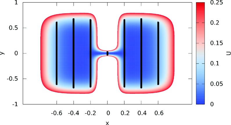
We consider the two-dimensional energy landscape discussed in Ref. 9. It consists of a double well potential with the basins connected through a narrow channel. This model for entropic barrier was used in the past to evaluate the quality of the Milestoning approximation.⁹ Here, we use the same model to evaluate the impact of the iterations on the accuracy and efficiency of the exact Milestoning algorithm. The potential energy (see Figure 4) is

$${\displaystyle U\left(x,y\right)=x^6+y^6+exp{\left(-x/\sigma \right)}^2\left[1-exp{\left(-y/\sigma \right)}^2\right].}$$ (47)

The numerical results shown below were computed with σ = 1/10.

FIG. 4.

A contour plot of the two-dimensional energy landscape that is used in the text to illustrate the exact Milestoning algorithm. We consider a transition from the well in the left to the well on the right. Also shown are the milestones (thick black lines). Note the narrow channel connecting the two wells. The channel does not include an energy barrier. Hence, the model considered is of an entropic barrier.

B. Model for the dynamics

For illustration purposes, we focus on a low dimensionality and a simple model that we can solve accurately. The two dimensional double well potential, which is described in III A, has this advantage. However, a complication of low dimensionality systems can be the lack of ergodicity. Milestoning requires ergodicity since the transition kernel must connect all states. To ensure ergodicity in the current test case, we use a stochastic model for the dynamics, overdamped Langevin

$${\displaystyle \frac{dz}{dt}=-\nabla U+R,}$$ (48)

where z is a two dimensional vector $z=\left(x,y\right)$ and R is a random force that follows the fluctuation dissipation theorem $〈R〉=0$ and $〈R\left(t\right)R\left(t^{\prime }\right)〉=2kT\delta \left(t-t^{\prime }\right)$. Milestoning can be used on a diverse set of ODEs and SDEs, including the overdamped Langevin equation. To solve Eq. (48) and obtain the coordinates z as a function of time, we used the BAOAB algorithm.³⁹ The temperature, kT, was 0.025 in all calculations with the exception of the study of the MFPT in which it was 0.008. The lower temperature helped us establish clearer dynamic characteristics of an activated process. However, the lower temperature requires more expensive calculations and we prefer to do the other studies at higher temperatures. The time step was Δt = 10⁻⁴. Straightforward long time trajectories from the initiating milestone to the last (absorbing) milestone were computed for comparison.

We consider a total of seven milestones defined as the hyperplanes (lines in this particular case),

$${\displaystyle M_i=\{(x,y)\in {\mathbb{R}}^2\hspace{0.17em}|\hspace{0.17em}x=-0.6+(i-1)\hspace{0.17em}\mathrm{\Delta }x\},}$$ (49)

where Δx = 0.2. The hyperplane M₁ is the initial milestone, while M₇ is the absorbing milestone.

IV. RESULTS AND DISCUSSIONS

A. Stationary flux and mean first passage time from exact Milestoning

Fig. 5 shows the estimates of the stationary flux (integrated over y and hence the same as the Milestoning weights, w, defined in Eq. (12)) for each milestone as functions of the number of iterations. Note that the scale does not start from zero and the errors are highly non-uniform. The convergence is considerably more rapid far from the absorbing boundary that distorts the initial guess of an equilibrium distribution at the milestone. Milestones 1-4 are near convergence after 10 iterations. Near the absorbing boundary more iterations are required with a maximum number of about 30.

FIG. 5.

Estimates for the components of the stationary flux vector at each iteration.

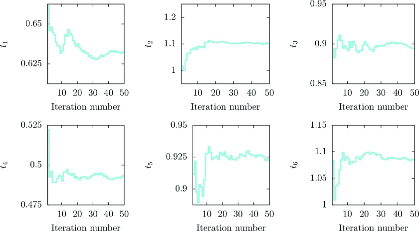
The estimated milestone lifetimes (the components of the vector t) as the iterations proceed are shown in Figure 6. Note that since the last milestone is absorbing, we never obtain an estimate for t₇. The range of times that we obtain is narrow and rapid convergence to the asymptotic value is observed. In a number of cases, essentially a single iteration brings us within ten percent of the converged value. Interestingly, the convergence of the local mean first passage time is less influenced by the proximity to the absorbing boundary in contrast to the calculation of the stationary flux.

FIG. 6.

Estimates for the local mean first passage times for the first six milestones. No estimate of the local MFPT can be provided for the final absorbing milestone (milestone 7).

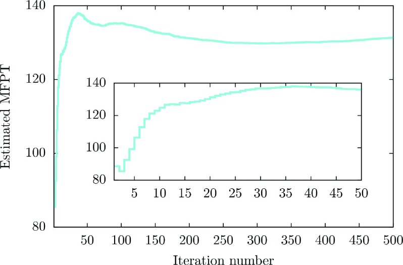
In Fig. 7 we show the overall mean first passage time as a function of the iteration number. The MFPT is computed according to Eq. (40). Note that the range of the MFPT values is narrow and it is possible to obtain a sound result with a relatively small number of iterations. The inset in the figure focuses on the first 50 iterations. Results within 15% of the final value can be obtained by ten iterations.

FIG. 7.

Estimated (global) mean first passage time. The inset provides the evolution of the estimate during the first 50 iterations of the algorithm.

The above calculations illustrate the convergence of the algorithm. It is useful to establish their correctness by conducting a study of the system using different computational means. We shall compare the ensembles of short trajectories used in Milestoning to long (uninterrupted) trajectories to verify the accuracy and efficiency of our procedure. This comparison is especially useful when considering the alternative of straightforward molecular dynamics simulations. However, the results of trajectory ensembles tend to be noisy, and similar to other stochastic sampling procedures, the averages converge relatively slowly with respect to the number of operations. It is therefore useful to compare the calculation to a significantly different computational approach with better convergence properties for the system at hand. The present test case is of low dimensionality. Systems of low dimensions can be studied accurately using numerical solutions of the Fokker-Planck equation. We describe a Fokker Planck solution of the model system and compare the results to Milestoning data below.

B. The Fokker-Planck solution

Consider the planar strips

$${\displaystyle {\mathrm{\Omega }{}_i}_{=}\left\{{(x,y)}^2\in {\mathbb{R}}^2\hspace{0.17em}|\hspace{0.17em}{x}_i-\mathrm{\Delta }x<x<x_i+\mathrm{\Delta }x\right\}.}$$ (50)

For each i = 1, …, 6, we see that the boundary ∂Ω_i of the ith strip is the disjoint union of the two milestones M_i−1 and M_i+1.

The survival probability of the system, denoted by S = S(x, y, t), is the solution of the initial-boundary value problem,

$${\displaystyle \left\{\begin{array}{cc}\hfill \frac{\partial S}{\partial t}(x,y,t)=\nabla \cdot J(x,y,t),\hfill & \hfill (x,y)\in {\mathrm{\Omega }}_i,t>0,\hfill \\ \hfill S(x,y,t)=0,\hfill & \hfill (x,y)\in \partial {\mathrm{\Omega }}_i,t\ge 0,\hfill \\ \hfill S(x,y,0)={\mathrm{g}}_i\text{(y)}\delta \left(x-x_i\right),\hfill & \hfill (x,y)\in {\mathrm{\Omega }}_i.\hfill \end{array}\right.}$$ (51)

The flux J is given by

$${\displaystyle J(x,y,t)={\beta }^{-1}\nabla S(x,y,t)+S(x,y,t)\nabla U(x,y)}$$ (52)

and S_i is a density function. The Milestoning calculation is conducted between milestones i = 1 and i = 7, the last milestone being absorbing. For the solution of the partial differential equation (PDE), which is conducted on a spatial grid, we add a reflective milestone M₀ that precedesM₁. No such reflective boundary was added for the trajectory calculations since the potential energy itself prevents the trajectories from reaching M₀. Since the probability of reaching M₀ is exceptionally small, the trajectory calculations in Milestoning and the solution of the Fokker-Planck equation on the grid are equivalent.

From the survival probability, we can obtain the density of the first hitting point distribution at the milestones M_i±1 by the formula

$${\displaystyle S_{i\pm 1}\left(y\right)={\int }_0^{\infty }\left|J_1(x_{i\pm 1},y,t)\right|\text{d}t.}$$ (53)

The non-zero entries of the transition matrix K are then K_M,1 = 1 and

$${\displaystyle K_{i,i\pm 1}=\frac{{\int }_{-\infty }^{\infty }{S}_{i\pm 1}\left(y\right)\hspace{0.17em}\text{d}y}{{\int }_{-\infty }^{\infty }(S_{i-1}\left(y\right)+S_{i+1}\left(y\right))\hspace{0.17em}\text{d}y}}$$ (54)

for i = 1,  …,  M − 1.

Hence, we can compare the transition matrix computed by the Brownian trajectories to the results of the partial differential equation. Our initial condition is a stationary flux distribution (determined by the Milestoning calculations) at only one interface and we run this distribution in time until the density terminates at the nearby milestones. The fraction of density that is accumulated at the nearby milestones determines the elements of the transition matrix. The transition matrix answers the question: given that we start from a particular milestone, what is the probability that the system will reach a particular (other) milestone at any time?

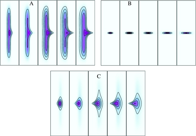
Time evolutions of densities computed with the Fokker Planck equation with the conditions described above are shown in Figure 8.

FIG. 8.

The time evolution of the probability density of a milestone. The simulation starts with the density at a milestone and is propagated in time using a solver for the partial differential equation. The density is absorbed at the nearby milestones and the simulation continues until it disappears. The results are used to estimate the probability of a transition to a particular milestone and the decay time. In the figure, the time dependent density is renormalized each step for clarity. A is for milestone at x = − 0.2, B for a milestone at x = 0, and C for a milestone at x = 0.2. Time progression is recorded from left to right. See text for more details.

C. A comparison between the Fokker Planck and exact milestoning solutions

For comparison, we consider the transition probabilities averaged over time and over the coordinate in the milestone. In the Milestoning language, we have

$${\displaystyle K_{\alpha \beta }=\underset{M_{\alpha },M_{\beta }}{\int }d{x}_{\alpha }d{x}_{\beta }\left[\underset{0}{\overset{\infty }{\int }}dt\cdot K_{\alpha \beta }\left(x_{\alpha },x_{\beta },t\right)\right]}$$ (55)

which is also the transition matrix used directly in the approximated version of the Milestoning theory.⁹

In Table I we compared the transition matrices, K_αβ, computed with exact Milestoning and by the Fokker Planck equation. It is obvious that the agreement is excellent.

TABLE I.

The transition matrix as a function of the milestone index.

The transition matrix Kαβ computed with exact Milestoning
0	1	0	0	0	0	0
0.3186	0	0.6814	0	0	0	0
0	0.9491	0	0.0509	0	0	0
0	0	0.4958	0	0.5042	0	0
0	0	0	0.0810	0	0.919	0
0	0	0	0	0.6806	0	0.3194
1	0	0	0	0	0	0
The transition matrix Kαβ computed with the Fokker Planck equation
0	1	0	0	0	0	0
0.3197	0	0.6821	0	0	0	0
0	0.9492	0	0.0508	0	0	0
0	0	0.4996	0	0.5004	0	0
0	0	0	0.0848	0	0.9152	0
0	0	0	0	0.6818	0	0.3182
1	0	0	0	0	0	0

In Table II we compare the weights of the stationary fluxes through the milestone (Eq. (15)). The agreement of the results from Milestoning and the Fokker-Planck equation is excellent. Of course, the stationary vectors are the eigenvectors of the transition matrix with the eigenvalue of one. Since the transition matrix is well reproduced, it is expected that the eigenvectors will be in agreement as well.

TABLE II.

The stationary flux as a function of the milestone index.

Exact Milestoning
0.1524	0.4556	0.3195	0.0183	0.0246	0.0226	0.0072
Fokker-Planck equation
0.1520	0.4558	0.3200	0.0183	0.0244	0.0223	0.0071

The lifetimes of the milestones measure how long it takes on average for a trajectory initiated on milestone α to reach (any) other milestone for the first time. Formally, it is defined as $t_{\alpha }\equiv \sum _{\beta }\underset{0^{-}}{\overset{\infty }{\int }}\underset{M_{\alpha }}{\int }\underset{M_{\beta }}{\int }t\cdot K_{\alpha \beta }\left(x_{\alpha },x_{\beta },t\right)d{x}_{\beta }\cdot d{x}_{\alpha }\cdot dt$. The lifetimes are compared in Table III. We remark that the milestone lifetime is a good estimator for the length of a trajectory that we will need to use in Milestoning and can be used to predict expected efficiency.

TABLE III.

Comparing the lifetimes of Milestones.

Computed with exact Milestoning
0.6304	1.0896	0.8985	0.4937	0.9261	1.0862	0
Computed with the Fokker-Planck equation
0.6224	1.0666	0.8850	0.5009	0.9104	1.0638	0

The overall MFPT, the time that it takes on average for a trajectory initiated at the first milestone to reach for the first time the absorbing milestone on the right, is 129.7525 in exact Milestoning and 129.4489 in the Fokker Planck solution. It is interesting that the MFPT is two orders of magnitude larger than the individual transition times, suggesting significantly higher efficiency in sampling a single transition event in Milestoning compared to a straightforward trajectory (in Milestoning, we only compute the trajectory fragments). Further evaluation of Milestoning efficiency is discussed in Sec. IV D.

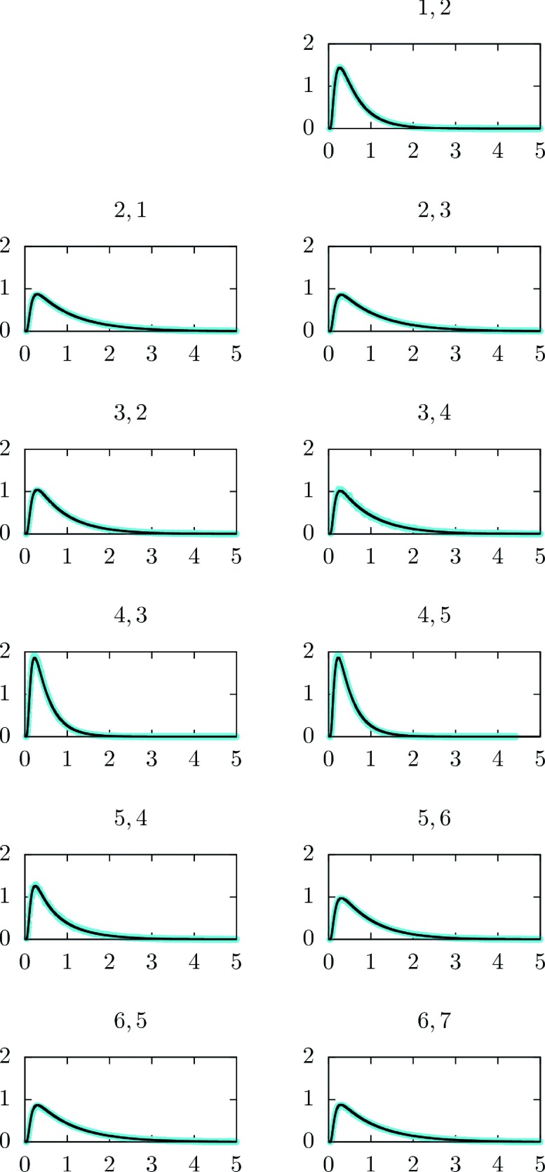
A more detailed picture is obtained when we considered the lifetimes as a function of the position in the milestone and between specific pairs of milestones. These distributions are shown in Figure 9. Again the agreement between Fokker Planck (solid black line) and blue dots (Milestoning) is excellent.

FIG. 9.

The probability densities of local transition times between pairs of milestones as a function of the transition time are shown. The indices of the milestones are indicated at the top of the panels. The black solid line is the solution of the Fokker Planck equation and the exact Milestoning are the blue dots.

In a Markovian process, the local transition times are distributed exponentially (without the delay time seen in all the distributions of Figure 9). The delays suggest that at the short time limit the Markovian assumption is violated. Indeed, we do not expect a master equation to be accurate at short times in the coarse space of the milestones.

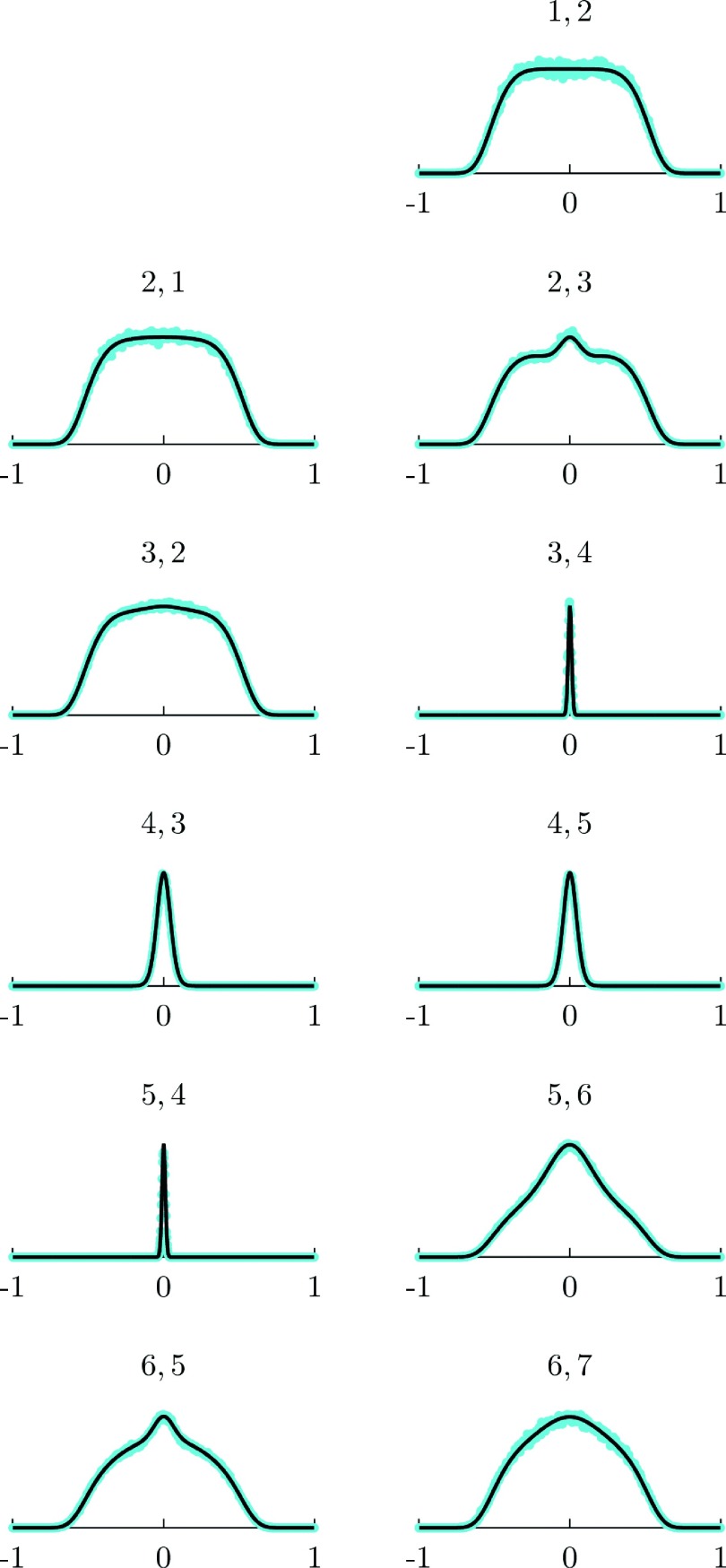
Other useful indicators of the dynamics are the stationary first hitting point distributions (FHPD) which are shown in Figure 10. The FHPD are obtained in the Fokker Planck equation by imposing absorbing boundaries at the nearby interfaces to the milestone on which trajectories were started.

FIG. 10.

First hitting distributions between pairs of milestones are shown as a function of the coordinate in the milestone line. The pairs are indicated at the top of the panel. The solid lines are the solutions of the Fokker Planck equation. The blue dots are the results of exact Milestoning calculations. The distributions are normalized to one. See text for more details.

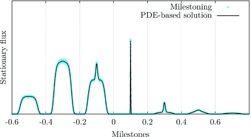
Another measure of accuracy is the convergence of the stationary flux. The stationary flux at individual milestones, computed with exact Milestoning, must be time independent also under the Fokker Planck formulation. Hence, if we provide to the Fokker Planck equation, the stationary fluxes of exact Milestoning as initial conditions and we propagate the spatial distribution as a function of time no spatial changes should be observed.

To show the convergence to the stationary flux distribution, we ran a simulation of exact Milestoning for up to 30 iterations and then took the resulting estimate q of the stationary flux as the initial conditions for the Fokker Planck equation in Eq. (51),

$${\displaystyle g_i\left(y\right)=\frac{S_i\left(y\right)}{\int S_i\left(y\right)\hspace{0.17em}\text{d}y}}$$

for the problems with i = 1,  …,  M. The resulting matrix K and first hitting distributions g_i can be used to obtain a new stationary flux vector q. This is akin to running an additional iteration of exact Milestoning where the first hitting distributions are obtained numerically by solving the partial differential equation for their densities. The estimate for the stationary flux obtained with Milestoning is indeed a fixed point of the transition operator as can be seen on Figure 11. The relative error in the L₁-norm between the estimated flux from Milestoning and the one coming from this additional iteration solving is equal to 0.0177.

FIG. 11.

Estimate for the stationary flux in the milestones compared with an additional iteration of exact Milestoning that solves the densities of the first hitting points by PDE methods. Note that the distributions are asymmetric with respect the origin at x since there is an absorbing boundary on the right.

We conclude that the accuracy obtained from the ensemble of trajectories in Milestoning is comparable to what we can get from the direct solution of the Fokker Planck equation.

In Sec. IV D, we compare the computational efficiency of exact Milestoning with long trajectories.

D. Comparison of Milestoning to long trajectories

A total of one hundred independent instances of each of the following two types of numerical experiments were conducted: uninterrupted trajectories from the first milestone on the left to the absorbing milestone on the right and Milestoning. For both types of experiments, we compute the mean first passage time to go from a point sampled from the canonical distribution conditioned to x = − 0.6 to any point at x = 0.6. We setup the system at a temperature of kT = 0.008 and used a time step length of Δt = 10⁻⁴ for the numerical integration of the trajectory fragments. In the uninterrupted trajectories, each independent experiment accumulates its own set of estimates for the first passage time and outputs the running average. For the Milestoning calculations, we setup milestones at the lines x = − 0.6, −0.55, −0.5, −0.4, −0.3, −0.2, −0.1, 0, 0.1, 0.2, 0.3, 0.4, 0.5, 0.55, and 0.6. From each of them we drew a total of 250 trajectory samples per iteration and we allowed the simulation to proceed for a total of 250 iterations.

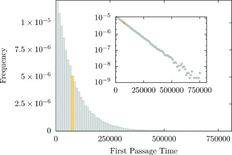
Each of the 108 815 individual samples of the first passage time obtained by the uninterrupted trajectories was collected in order to compute an empirical distribution for the FPTs whose details are found in Figures 12 and 13.

FIG. 12.

Histogram of empirical distribution of first passage times. The bar highlighted in yellow is the numerical estimate of the MFPT. In the inset, we plot the same data on logarithmic scale to emphasize the exponential nature of the distribution.

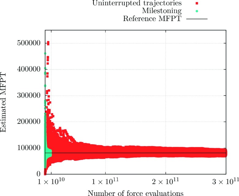
FIG. 13.

Running averages coming from both types of experiments. The black line is the best numerical estimate for the MFPT. The distribution of the dots show the running average for the 100 repeats of the calculation either for long trajectories (red) or Milestoning (blue).

To check the efficiency of the calculation, it is useful to examine running averages. We consider the MFPT as a function of the number of force evaluations. Every time step requires one force evaluation. In molecular dynamics simulations, the calculations of the forces are the most time consuming operation per step. The running average of the MFPT is shown in Figure 13.

Observe that there are very few samples of the running MFPT coming from uninterrupted trajectories below 10¹⁰ force evaluations. Due to this lack of samples, the statistics are poor. However, the Milestoning runs sample significantly the MFPT for this range of force evaluations.

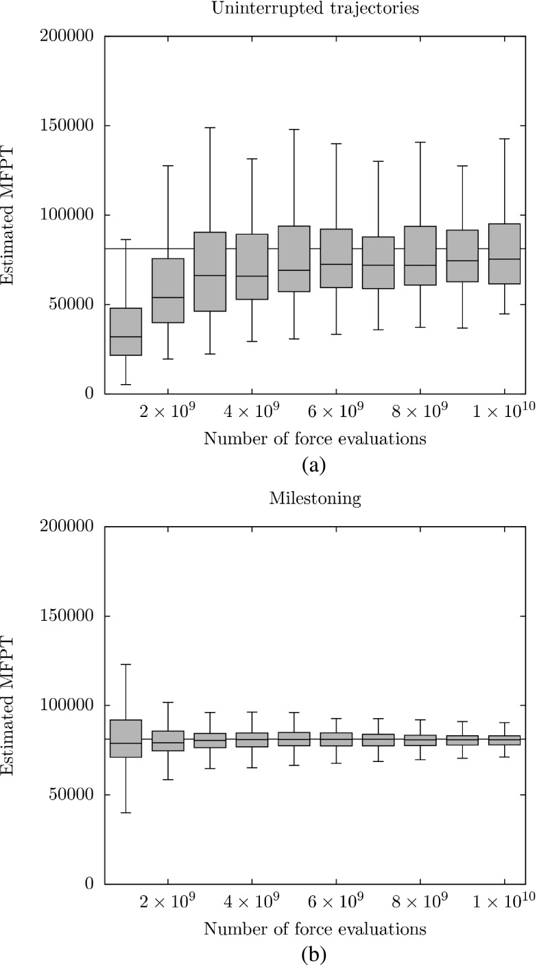
Further information about the error and the convergence is provided in Figures 14(a) and 14(b). These figures use box plot representations to illustrate the changes in the MFPT as a function of the number of force evaluations.

FIG. 14.

(a) Box plots for MFPTs obtained from uninterrupted trajectories. The horizontal line is the best estimate for the MFPT. (b) Box plots for MFPTs obtained from Milestoning.

From the above plots, it is evident that Milestoning is significantly more efficient than straightforward molecular dynamics even in a case without an energy barrier (the barrier in our example is entropic).

E. Dependence on the initial guess

Milestoning is an iterative solution of vector-matrix operation that determines an eigenvector with an eigenvalue one. The speed of convergence depends on the initial guess of the eigenvector. Here, we consider this dependence. In the first version of Milestoning,⁹ the distribution at the interface was taken from equilibrium. We use the same initial condition here. Now we also consider an extreme case in which the whole population is concentrated at the first milestone and then propagated with iterations throughout the system. The last choice mimics the calculations in the Forward Flux Sampling (FFS) algorithm.⁴⁰

We consider again the same set of seven milestones M₁,  …, M₇ that were used in previous experiments. We started a total of 100 trajectory fragments per (relevant) milestone per iteration for a total of 500 iterations.

In this case, we used reflecting boundary conditions at the last milestone. This yields a symmetric stationary flux distribution due to the last row of the transition matrix being K_7,k = δ_6,k.

In Figure 15 we show the convergence of the flux as a function of the iteration number. It is obvious that 500 iterations were not required and that starting from the canonical distribution is a much faster algorithm. Nevertheless, the efficiency of the algorithm starting from a single initiating milestone is not too bad. It suggests that one could use the exact Milestoning procedure to compute non-equilibrium process in which the distributions at nearby milestones are built on the fly. The only input is the milestone we start from.

FIG. 15.

Local convergence of each flux distribution. For each milestone, we use the error measurement ${‖q_i^n-q_i^{n-1}‖}_{\infty }/{‖q_i^n‖}_{\infty }$ to highlight the maximum discrepancy between the current and the previously obtained flux distribution. The red line corresponds to the experiment in which all the trajectories are initially at the first milestone while the blue line shows the corresponding results for the experiment in which trajectories are initially sampled from all milestones according to the Boltzmann distribution.

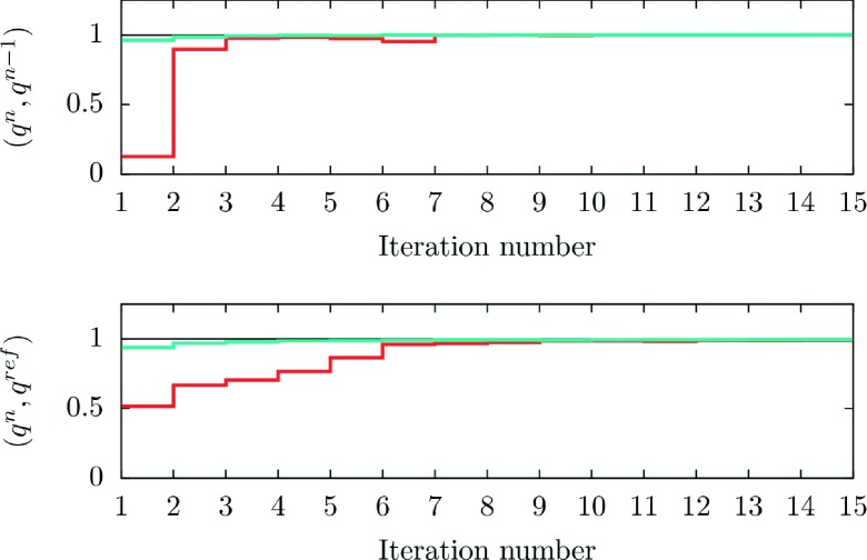
Global convergence is shown in Figure 16 illustrating again faster convergence of the thermally distributed “old Milestoning” initial guess.

FIG. 16.

Global convergence results using Rayleigh quotients. The figure on the top displays the inner products (appropriately normalized) of the flux distributions qⁿ⁻¹ and qⁿ. The graph on the bottom shows the inner product for the current iteration qⁿ and the reference flux q^ref = q⁵⁰⁰. Again, the red color corresponds to the experiment where the initial trajectories are started only at the first milestone while the blue color is for the experiment where we initially run trajectories from every milestone assuming canonical distribution at each milestone.

V. SUMMARY

We have introduced a new variant of Milestoning, which is exact (subject to converged sampling). This variant proposed a new way of computing kinetics and thermodynamics from trajectories using as a guideline a mesh of Voronoi cells. Since short trajectories are computed over a limited spatial range, the algorithm avoids many of the ergodicity problems of straightforward MD and trapping in metastable states. Of course, this conceptual gain is not coming completely for free and some initial guesses and exploratory simulations are necessarily to identify plausible locations of the Voronoi cells. However, if such a sample is available (the center of the Voronoi cells, the anchors, can be obtained by high temperature trajectories, for example) the gain in efficiency and convergence is profound. Essentially, a complete picture of the statistical mechanics of the system is obtained at reduced cost.

The algorithm is based on iterative determination of stationary flux vectors at milestones. The stationary fluxes are elements of the eigenvector of the transition matrix with an eigenvalue one. The transition matrix (in contrast to the prior versions of Milestoning) is not computed explicitly. Instead, we consider the products of this matrix times a vector, which is the current iteration and estimate of the stationary flux. The vector-matrix products are conducted repeatedly to generate an iterative solution to the flux vector. The properties of the transition matrix guarantee convergence of the iteration process under mild conditions.

We illustrate that the algorithm is significantly more efficient than straightforward MD, which is not surprising since the earlier approximate versions of Milestoning were already much more efficient than MD. The older version of Milestoning is essentially a single iteration of the exact Milestoning procedure. The iterations make the exact version between 10 and 100 times slower in the current implementation. This still leaves ample speedup of exact Milestoning compared to straightforward MD. Because of the relatively short distances between milestones and the short duration of the trajectories, the calculations are not very sensitive to the structure of the energy landscape. This is because at short distances and times the variations in the energy landscape are small.

Also encouraging is the observation that the approximate version of Milestoning that uses only a single iteration is quite reasonable for the example presented and provides results that are not too far from the exact answer.

Nevertheless, we comment that the exact and full determination of the flux vector in Milestoning (if desired) remains a challenge. It is a very long vector of length of the number of milestones times the number of phase space points within a milestone. So, while we have an exact linear equation for it, an exact solution of the flux vector at high dimension is not possible. The more likely scenario is the use of sampling to compute averages and integrals that rely on q for sampling in the milestone. For increased accuracy of estimates of the flux that goes beyond the canonical weight of the zero order iteration (Eq. (11)), trajectory fragments can be computed in the forward and backward direction like in directional Milestoning.¹⁶ This is similar in spirit to the methods of PPTIS⁷ and to the Milestoning with memory.³² Also, similar to the approach taken in the Markov state model,⁴¹ full trajectories from reactants to products, if available, can be analyzed for crossing events and the exact Milestoning theory can be used to extract kinetics and thermodynamics. For the case of full exact trajectories, the sampling of the flux vector at the milestone is done from the exact distribution.

More can be done to increase the efficiency of the Milestoning algorithm and work in that direction is in progress. For example, the sampling in a milestone need not be uniform and it depends on the level of convergence achieved locally. The local sampling at milestones, which is trivially parallelizable, can be optimized to ensure better distributions of effort. Addition and subtraction of milestones can be automated to take into account newly discovered domains of the coarse variables. A useful work in that direction can be found in Ref. 42.

REFERENCES

- 1.Shaw D. E., Deneroff M. M., Dror R. O., Kuskin J. S., Larson R. H., Salmon J. K., Young C., Batson B., Bowers K. J., Chao J. C., Eastwood M. P., Gagliardo J., Grossman J. P., Ho C. R., Ierardi D. J., Kolossvary I., Klepeis J. L., Layman T., McLeavey C., Moraes M. A., Mueller R., Priest E. C., Shan Y. B., Spengler J., Theobald M., Towles B., and Wang S. C., Commun. ACM 51(7), 91-97 (2008). 10.1145/1364782.1364802 [DOI] [Google Scholar]
- 2.Austin R. H., Beeson K. W., Eisenstein L., Frauenfelder H., and Gunsalus I. C., Biochem. 14(24), 5355-5373 (1975). 10.1021/bi00695a021 [DOI] [PubMed] [Google Scholar]
- 3.Olender R. and Elber R., J. Chem. Phys. 105(20), 9299-9315 (1996). 10.1063/1.472727 [DOI] [Google Scholar]
- 4.Bolhuis P. G., Chandler D., Dellago C., and Geissler P. L., Annu. Rev. Phys. Chem. 53, 291-318 (2002). 10.1146/annurev.physchem.53.082301.113146 [DOI] [PubMed] [Google Scholar]
- 5.Swenson D. W. H. and Bolhuis P. G., J. Chem. Phys. 141(4), 044101 (2014). 10.1063/1.4890037 [DOI] [PubMed] [Google Scholar]
- 6.Elber R. and Karplus M., Science 235(4786), 318-321 (1987). 10.1126/science.3798113 [DOI] [PubMed] [Google Scholar]
- 7.Moroni D., Bolhuis P. G., and van Erp T. S., J. Chem. Phys. 120(9), 4055-4065 (2004). 10.1063/1.1644537 [DOI] [PubMed] [Google Scholar]
- 8.Zhang B. W., Jasnow D., and Zuckerman D. M., J. Chem. Phys. 132(5), 054107 (2010). 10.1063/1.3306345 [DOI] [PMC free article] [PubMed] [Google Scholar]
- 9.Faradjian A. K. and Elber R., J. Chem. Phys. 120(23), 10880-10889 (2004). 10.1063/1.1738640 [DOI] [PubMed] [Google Scholar]
- 10.Czerminski R. and Elber R., J. Chem. Phys. 92(9), 5580-5601 (1990). 10.1063/1.458491 [DOI] [Google Scholar]
- 11.Fichthorn K. A. and Lin Y. Z., J. Chem. Phys. 138(16), 164104 (2013). 10.1063/1.4801869 [DOI] [PubMed] [Google Scholar]
- 12.Kirmizialtin S. and Elber R., J. Phys. Chem. A 115(23), 6137-6148 (2011). 10.1021/jp111093c [DOI] [PMC free article] [PubMed] [Google Scholar]
- 13.Kreuzer S. M., Elber R., and Moon T. J., J. Phys. Chem. B 116(28), 8662-8691 (2012). 10.1021/jp300788e [DOI] [PMC free article] [PubMed] [Google Scholar]
- 14.Kirmizialtin S., Nguyen V., Johnson K. A., and Elber R., Structure 20(4), 618-627 (2012). 10.1016/j.str.2012.02.018 [DOI] [PMC free article] [PubMed] [Google Scholar]
- 15.Vanden-Eijnden E. and Venturoli M., J. Chem. Phys. 130(19), 194101 (2009). 10.1063/1.3129843 [DOI] [PubMed] [Google Scholar]
- 16.Majek P. and Elber R., J. Chem. Theory Comput. 6(6), 1805-1817 (2010). 10.1021/ct100114j [DOI] [PMC free article] [PubMed] [Google Scholar]
- 17.Dickson A., Warmflash A., and Dinner A. R., J. Chem. Phys. 130(7), 074104 (2009). 10.1063/1.3070677 [DOI] [PubMed] [Google Scholar]
- 18.Warmflash A., Bhimalapuram P., and Dinner A. R., J. Chem. Phys. 127(15), 154112 (2007). 10.1063/1.2784118 [DOI] [PubMed] [Google Scholar]
- 19.Vanden-Eijnden E. and Venturoli M., J. Chem. Phys. 131(4), 044120 (2009). 10.1063/1.3180821 [DOI] [PubMed] [Google Scholar]
- 20.Kubo R., Toda M., and Hashitsume N., Statistical Physics II: Nonequilibrium Statistical Mechanics (Springer Verlag, Berlin, 1978). [Google Scholar]
- 21.Czerminski R. and Elber R., Int. J. Quantum Chem. 38, 167-186 (1990). 10.1002/qua.560382419 [DOI] [Google Scholar]
- 22.Olender R. and Elber R., J. Mol. Struct.: THEOCHEM 398, 63-71 (1997). 10.1016/S0166-1280(97)00038-9 [DOI] [Google Scholar]
- 23.Elber R., Biophys. J. 92(9), L85-L87 (2007). 10.1529/biophysj.106.101899 [DOI] [PMC free article] [PubMed] [Google Scholar]
- 24.Elber R. and West A., Proc. Natl. Acad. Sci. U. S. A. 107, 5001-5005 (2010). 10.1073/pnas.0909636107 [DOI] [PMC free article] [PubMed] [Google Scholar]
- 25.Kreuzer S. and Elber R., Biophys. J. 105(4), 951-961 (2013). 10.1016/j.bpj.2013.05.064 [DOI] [PMC free article] [PubMed] [Google Scholar]
- 26.Jas G. S., Hegefeld W. A., Majek P., Kuczera K., and Elber R., J. Phys. Chem. B 116(23), 6598-6610 (2012). 10.1021/jp211645s [DOI] [PMC free article] [PubMed] [Google Scholar]
- 27.Cardenas A. E. and Elber R., J. Chem. Phys. 141(5), 054101 (2014). 10.1063/1.4891305 [DOI] [PMC free article] [PubMed] [Google Scholar]
- 28.Cardenas A. and Elber R., Mol. Phys. (to be published).
- 29.Kreuzer S. M., Moon T. J., and Elber R., J. Chem. Phys. 139(12), 121902 (2013). 10.1063/1.4811366 [DOI] [PMC free article] [PubMed] [Google Scholar]
- 30.Cardenas A. E. and Elber R., Mol. Phys. 111(22-23), 3565-3578 (2013). 10.1080/00268976.2013.842010 [DOI] [PMC free article] [PubMed] [Google Scholar]
- 31.Golub G. H. and Van Loan C., Matrix Computation, 4th ed. (Johns Hopkins University Press, Baltimore, 2012). [Google Scholar]
- 32.Hawk A. T. and Makarov D. E., J. Chem. Phys. 135(22), 224109 (2011). 10.1063/1.3666840 [DOI] [PubMed] [Google Scholar]
- 33.Viswanath S., Kreuzer S. M., Cardenas A. E., and Elber R., J. Chem. Phys. 139(17), 174105 (2013). 10.1063/1.4827495 [DOI] [PMC free article] [PubMed] [Google Scholar]
- 34.West A. M. A., Elber R., and Shalloway D., J. Chem. Phys. 126(14), 145104 (2007). 10.1063/1.2716389 [DOI] [PubMed] [Google Scholar]
- 35.Hawk A. T., J. Chem. Phys. 138(15), 154105 (2013). 10.1063/1.4795838 [DOI] [PubMed] [Google Scholar]
- 36.Nuske F., Keller B. G., Perez-Hernandez G., Mey A., and Noe F., J. Chem. Theory Comput. 10(4), 1739-1752 (2014). 10.1021/ct4009156 [DOI] [PubMed] [Google Scholar]
- 37.Vanden Eijnden E., Venturoli M., Ciccotti G., and Elber R., J. Chem. Phys. 129(17), 174102 (2008). 10.1063/1.2996509 [DOI] [PMC free article] [PubMed] [Google Scholar]
- 38.Reimann P., Schmid G. J., and Hanggi P., Phys. Rev. E 60(1), R1-R4 (1999). 10.1103/PhysRevE.60.R1 [DOI] [PubMed] [Google Scholar]
- 39.Leimkuhler B. and Matthews C., J. Chem. Phys. 138(17), 174102 (2013). 10.1063/1.4802990 [DOI] [PubMed] [Google Scholar]
- 40.Allen R. J., Frenkel D., and ten Wolde P. R., J. Chem. Phys. 124(2), 024102 (2006). 10.1063/1.2140273 [DOI] [PubMed] [Google Scholar]
- 41.Schutte C., Noe F., Lu J. F., Sarich M., and Vanden-Eijnden E., J. Chem. Phys. 134(20), 204105 (2011). 10.1063/1.3590108 [DOI] [PubMed] [Google Scholar]
- 42.Shalloway D. and Faradjian A. K., J. Chem. Phys. 124(5), 054112 (2006). 10.1063/1.2161211 [DOI] [PubMed] [Google Scholar]