

Abstract
The resurgence of pulsed electron paramagnetic resonance (EPR) in structural biology centers on recent improvements in distance measurements using the double electron-electron resonance (DEER) technique. This unit focuses on EPR-based distance measurements by site-directed spin-labeling (SDSL) of engineered cysteine residues in soluble proteins, with HIV-1 protease used as a model. To elucidate conformational changes in proteins, experimental protocols were optimized and existing data analysis programs were employed to derive distance distribution profiles. Experimental considerations, sample preparation and error analysis for artifact suppression are also outlined here.
Keywords: Pulsed EPR, DEER, distance measurements, site-directed spin-labeling
INTRODUCTION
There are four common EPR techniques utilized to interrogate specific distance ranges: exchange EPR for short distances in the 4–8 Å range (Miick et al., 1992), continuous-wave (CW) EPR for distances of 8–25 Å (Rabenstein and Shin, 1995; McHaourab et al., 1997; Cooke and Brown, 2011) and two pulsed methods that cover distances from 15–80 Å: double electron-electron resonance (DEER), also known as pulsed electron double resonance (PELDOR) (Tsvetkov and Grishin, 2009; Jeschke, 2012) and double quantum coherence (DQC) (Borbat et al., 2002; Misra et al., 2009). Distance measurements by site-directed spin-labeling (SDSL) EPR are based on the dependence of the electron dipole-dipole couplings, which scale as 1/r3, where r is distance between unpaired spins. The first technique, exchange EPR, relies on the overlap of two unpaired electron orbitals and dipole-dipole broadening between the electron spins. Meanwhile, in CW EPR methods, distances are obtained by analyzing the line width increases that result from the dipole-dipole interactions (Rabenstein and Shin, 1995; Altenbach et al., 2001). The distances are then obtained from a Fourier transform deconvolution to extract the Pake broadening function, which is simulated in terms of the distances and distance distributions that generated the Pake function. The upper limit of 20–25 Å for traditional nitroxide spin labeling experiments is set by the inherent inhomogeneous broadening of the nitroxide spectrum. This limit can be extended by deuterating the spin label or by using a spin label with a narrower line shape. Typically, when measuring distances in the 20–80 Å range, pulsed EPR techniques are utilized (Pannier et al., 2000; Borbat et al., 2002; Borbat et al., 2004; Jeschke et al., 2004b; Jeschke et al., 2006; Jeschke and Polyhach, 2007). The four-pulse DEER methodology determines the dipolar coupling between spins in the form of a modulation of the spin echo amplitude, with great sensitivity in the range of 20–80 Å, achieving a precision of 0.3 Å for the lower end of this range (Pannier et al., 2000; Jeschke, 2002; Galiano et al., 2009b). In DQC, another pulsed EPR technique, the dipole interactions between spins generates double quantum coherences, where the rate of formation of the coherence directly reports on the strength of the dipolar interaction (Borbat et al., 2002; Borbat et al., 2004).
Either extrinsic or intrinsic EPR-active species can be utilized in distance measurements. The former are artificially introduced, such as nitroxide radicals or metal centers chelated at targeted specific sites, whereas the latter are unpaired electrons that exist naturally in proteins, such as amino acid radicals, paramagnetic metals and radical cofactors. DEER has been utilized in a variety of biomolecules, such as peptides (Milov et al., 1999), proteins with tyrosyl radicals (Bennati et al., 2003), soluble proteins (Persson et al., 2001), integral membrane proteins (Jeschke et al., 2004c) and nucleic acids (Cai et al., 2007; Kim et al., 2010). Distance measurements with DEER are not limited to nitroxides; distances between metal centers, such as Cu2+-Cu2+ (Yang et al., 2007); between iron paramagnets in FeS clusters (Roessler et al., 2010), Gd3+-Gd3+ (Raitsimring et al., 2007; Potapov et al., 2010) and between metal and spin-label, such as Cu2+-nitroxide (Narr et al., 2002; Yang et al., 2010) and iron-sulfur center-nitroxide (Lovett et al., 2009) pairs have also been explored. This list serves to provide select examples and is in no way inclusive of the numerous papers published in this discipline.
Although distances up to 60–80 Å can be achieved for soluble proteins with matrix deuteration, the limit falls to 40–45 Å for membrane proteins, as fast relaxation times often do not allow for dipolar evolution times exceeding 1.8–2.0 μs (Dastvan et al., 2010). In addition to using alternative spin markers for protein labeling, such as Gd3+, sensitivity of the DEER experiment on conventional nitroxide radicals can potentially be enhanced by going to higher frequencies. Assuming that the experiment can be done under otherwise the same conditions, pulsed EPR sensitivity scales with the square of the resonance frequency (Borbat et al., 1997), implying about 13- and 100-fold sensitivity gain when going from X to Q and W bands; respectively. Consequently, for Q-band, a 169-fold decrease in data acquisition time has been achieved (Ghimire et al., 2009). However, such enhancement in absolute sensitivity does not necessarily translate to better concentration sensitivity due to smaller sample volumes and lower excitation power at higher frequency.
Here, we outline important experimental considerations for DEER data collection and analysis, which our lab has utilized for nitroxide-based DEER studies of HIV-1 protease, and is compatible with distance measurements in other soluble proteins in the 20–50 Å range. This protocol is applicable to a Bruker EleXsys E580 instrument operating at X-band (8–12 GHz) and equipped with the ER 4118X-MD-4/ER 4118X-MD-5 dielectric ring resonator using a four-pulse DEER sequence. When alternative considerations are needed for SDSL DEER, such as for membrane protein samples, comments are given and additional references are provided.
Nitroxide Spin Labels
By definition, a spin label is any molecule containing an unpaired electron and reactive moiety for binding to another molecule. Most of the spin labels employed for studying structure and flexibility of biomolecules are nitroxide radicals because their simple line shape is highly sensitive to motion, making them ideal for such investigations (Fajer, 2000). The nitroxide radicals for spin labeling applications are persistent because the electron is protected by bulky methyl groups that sterically prevent collisions, and hence limit the reactivity of the radical. The geometry of the radical and surrounding methyl groups is typically preserved by inclusion in a five-membered pyrrole ring or six-membered piperidine ring. Pyrrole rings with an unsaturated bond have lower flexibility. Many versions of nitroxide spin labels have been generated by Kalman Heidig and the popularity of these labels has led to their commercial availability from Toronto Research Chemicals.
Commercially available spin labels vary in both their ring structure and in their reaction chemistry for attachment to the protein. Figure 1 shows the structures of four common nitroxide radicals with thiol-based linkers, as well as the structures of the modified cysteine after reacting with the spin label. Unlike other nitroxide spin labels, the unnatural, conformationally restricted nitroxide amino acid, 2,2,6,6-tetramethyl-N-oxyl-4-amino-4-carboxylic acid (TOAC) readily adopts helical backbone torsion angles and is incorporated as a rigid spin label during peptide synthesis (Hanson et al., 1998; Schreier et al., 2012). Biradical nitroxide labels with linkers of different flexibility have also been used in membrane protein studies (Polyhach et al., 2012). Recently, the use of a triarylmethyl-based spin label with a relatively long relaxation time enabled pulsed EPR distance measurements in a protein immobilized to a solid support (Yang et al., 2012).
Figure 1.

Chemical structures of four common nitroxide spin-labels before and after reacting to a cysteine side chain. A) and B) MTSL: (1-oxyl-2,2,5,5-tetramethyl-Δ3-pyrroline-3-methyl) methanethiosulfonate; C) and D) IAP: 3-(2-iodoacetamido)-proxyl; E) and F) MSL: 4-maleimido-TEMPO; and G) and H) IASL: 4-(2-iodoacetamido)-TEMPO. The rectangular box represents the protein backbone.
Selection of Labeling Sites
The choice of labeling sites within biological systems is not trivial. Obviously, the site should be chosen to report on the relevant aspect of the system under study. However, the introduction of the spin label should not alter the structure, stability or function of the system, and functional assays of the modified proteins are essential components to any SDSL EPR study. For distance measurements, a solvent-exposed reporter site is preferred over a buried site because it is less likely to produce structural perturbation due to its presence. It has also been noted that the extent of solvent exposure at the selected site impacts the distance distribution profile (Altenbach et al., 2008). For solvent exposed sites, the spin label has conformational rotational freedom dictated by the structure of the spin label, which often has averaged conformational sampling. Oftentimes, spin labels in buried sites or site of tertiary contact adopt multiple conformations, which can complicate analysis of distance distribution profiles. A solvent exposed site with minimal contacts is often considered an optimum labeling site for distance measurements because the spin label adopts a limited number of rotamers (Altenbach et al., 2008).
An important complement to any DEER experiment is the use of computational simulations, both for protein conformational sampling (Durrant and McCammon, 2011) and likely spin label rotamers at the chosen site in a protein (Polyhach et al., 2011). These studies are often necessary when building a biological model around the experimentally observed distances and distance changes, and determining favorable spin-labeling sites (Polyhach and Jeschke, 2010). An open-source software MMM 2011.2, available from the Swiss Federal Institute of Technology Zurich website (http://www.epr.ethz.ch), allows in-silico incorporation of spin labels and model-based fitting of conformational changes in proteins. With this program, provided that the initial structural conditions and a set of probable distance constraints for the chosen spin label are known, predictions for the structure following labeling can be made.
Commonly, nitroxide spin labels (SL) are covalently linked to proteins at specific amino acid residues. The functional group attached to the nitroxide provides specificity to the labeling reaction. In particular, cysteine residues are targeted by iodoacetamide, maleimide, indanedione and α-ketone functional groups attached to the nitroxide moiety, while activated esters are specific to lysines. Nitroxide probes are often used as extrinsic spin labels in SDSL (Hubbell et al., 1998). Here, native cysteines are typically replaced with another amino acid, such as alanine or serine depending upon the relative hydrophobicity of the local site, and new cysteine residues are engineered at specific positions. Sulfhydryl-specific spin labels are then attached to the cysteine residues.
The linker by which nitroxide probes conjugate to the protein confers an intrinsic conformational flexibility. To reduce probe flexibility, MTSL has been modified in the 4-position of the pyrrole ring to include bulky groups such as phenyl (Fawzi et al., 2011) or bromo moieties (Altenbach et al., 2001; Pistolesi et al., 2007; Georgieva et al., 2012), and the latter MTSL analogue (4-bromo-MTSL) is commercially available. Additional restriction of spin label motion can be incorporated by bifunctional SL that enable cross linking of two target sites on a peptide or protein (Fleissner et al., 2011). Alternatively, rigid unnatural amino acid spin labels can be incorporated into the backbone at specific sites of the polypeptide chain during peptide synthesis, in the case of TOAC (Hanson et al., 1998) or by using an elegant method of unnatural amino acid mutagenesis (Cornish et al., 1994).
Distance Measurements via DEER
Figure 2 illustrates the pulse sequence used for four-pulse DEER (Jeschke, 2012). In DEER experiments, microwave pulses are used to selectively excite two distinct spin populations (generally referred to as spins A and B). The B spins are flipped, which perturbs the coupled A spins, resulting to a modulation on the A spins. The sequence begins with a two-pulse Hahn echo sequence on ωmwA. After the appearance of the Hahn echo, a pump pulse is applied on ωmwB with a varying time delay after the echo. At τ2, the echo is refocused by an additional π-pulse on ωmwA. Again, the echo intensity is recorded as a function of the time delay between the first echo and the pump pulse.
Figure 2.
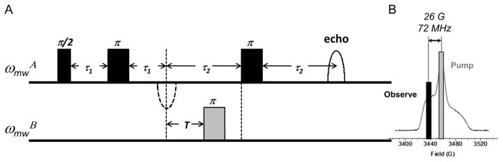
(A) Four-pulse DEER. Each pulse delay labeled with τ remains constant while spacing labeled with T is incremented. (B) Pump and observe frequencies for nitroxide labels at X-band.
The pump pulse flips the B spins at time T, which alters the effective magnetic field of the A spins that are coupled to the B spins. This change in the magnetic field changes the precession frequency of the coupled spins via electron-electron coupling (ωee), which results in the magnetization being out of phase by the angle Δϕee=ωeeT. Thus, ωee can be determined by integrating the echo intensity as a function of T. Equation 1 defines ωee,
| (Equation 1) |
where rAB is the distance between the spins, θAB is the angle subtended by the static field Bo and the vector between the spins, J is the exchange coupling, and ωdd is the dipolar coupling between the electrons. Equation 1 is valid as long as the positions of the electron spins are relatively well-defined in relation to the distance between them, such that the point-dipole approximation holds (Riplinger et al., 2009). This restriction is easily met for spins more than 15 Å apart, which is the lower limit for a DEER experiment. The J-coupling is significant only at short distances and considered negligible for distances greater than 20 Å (Jeschke and Polyhach, 2007).
In four-pulse DEER, ωmwA is the observe frequency (corresponding to A spins) and ωmwB is the pump frequency (B spins). Both frequencies are chosen such that there is no overlap (or minimal overlap) between the excitation windows of the pulses and that the highest number of spins is excited. For nitroxide labels at X-band, the low- and center-field transitions are ~26 G apart (which corresponds to ~72 MHz) as shown in Figure 2B. Typically, the pump frequency is chosen to correspond to the center-field transition because it is the most populated region of the spectrum. Meanwhile, the low-field manifold, which is the second most populated region, is often selected as the observe frequency. However, any position along the powder spectrum can be chosen for either the pump or probe pulses as long as the frequencies are well-separated, so as to prevent exciting A spins with B pulses and vice-versa. For split-ring or loop-gap resonators, it could be advantageous to situate the pump pulse to the resonator dip and to increase the observed frequency so as to compensate for the limited pumping power (Fajer et al., 2006). Note that experiments performed at higher frequencies (i.e., Q-band or W-band) follow this same procedure (Raitsimring et al., 2007; Potapov et al., 2010; Polyhach et al., 2012). However, as the field strength increases, the anisotropy of the powder spectrum is altered. For nitroxide labels at X-band, the anisotropy of the hyperfine tensor dominates the shape of the powder spectrum; whereas at W-band the g-tensor anisotropy dominates. The frequency offsets chosen will be dictated by the frequency of the experiment. Additionally, these offsets and powder spectra will differ when metals are used as the spin label, as g-tensor anisotropy may dominate even at X-band (Yang et al., 2007; Potapov et al., 2010).
The DEER method is intrinsically insensitive. The DEER pulse sequence utilizes frequencies that are selective to given orientations of spin labels in the sample. The ‘powder’ nature of the spectrum is indicative of a ‘frozen’ sample where there is limited motional rearrangement of the molecules during the time of the experiment. Because the pulses are ‘selective’, this means only a small fraction of the total sample will be excited by the pulse. Furthermore, given the random powder orientation of the sample, only a fraction of the protein molecules in the sample will have the magnetic components of the nitroxide radical that is oriented so they match the orientation selection of the A and B spins dictated by the pulse sequence frequency offsets. Inspection of the echo-detected powder pattern spectrum in Figure 2B reveals that majority of spins are neither A nor B spins (portions of spectrum not highlighted). Additionally, the practical concern of incomplete sample spin labeling could further reduce the signal intensity. Although the selective pulses lead to inherently lower signals, a benefit of the frequency offsets is the ability to perform orientation selection for spin-labels, which has great advantages in spin-labeling of nucleic acids as well as distance determination in metals (Schiemann et al., 2009).
The total DEER signal detected arises from both the intramolecular distance of interest as well as contributions from signals of all other random intermolecular interactions. Given a frozen protein sample, each of the desired A spins may have an intramolecular B spin for interrogation, but it will also be surrounded by other spins on neighboring proteins, some of which will also be B spins. These intermolecular interactions give rise to a background signal, which comes from a random distribution of large distances, which can usually be modeled by an exponential decay (Jeschke et al., 2004b). The total signal, which is a combination of both intra- and intermolecular distances, takes the form of a damped oscillation, as shown in Figure 3. In this illustration, the raw dipolar evolution curve is shown as the solid gray line. This signal is usually designated as V(t). The background contribution is plotted as a dashed blue line and is represented by B(t). The background corrected signal, F(t) is plotted as a solid black line. The relationship between the signal, the background, and the background-corrected signal is given by Equation 2. The decay time for the oscillations in F(t), τdecay, and the maximum dipolar evolution time, τmax, are also shown in Figure 3. The modulation depth λ is a correction factor that compensates for the incomplete excitation of all B spins by the pump pulse.
Figure 3.

Sample dipolar evolution curve before (gray solid line) and after (black solid line) applying the background subtraction function (blue dashed line). The red line is the regenerated echo curve from data analysis, which is discussed in Basic Protocol 4.
| (Equation 2) |
In the protocols that follow, Basic Protocol 1 describes site-directed spin-labeling of soluble proteins, which is usually accomplished via an engineered cysteine residue. In Basic Protocol 2, the preparation of DEER samples is described, which involves buffer exchange by concentration or dialysis and addition of cryoprotectants. EPR spectrometer set-up, preliminary experiments and DEER data acquisition are described in Basic Protocol 3, and the subsequent DEER data analysis to derive distance information from dipolar evolution curves is described in detail in Basic Protocol 4.
BASIC PROTOCOL 1: Site-directed Spin-labeling of Soluble Proteins
BASIC PROTOCOL 2: Preparing DEER Samples
BASIC PROTOCOL 3: Setting up the EPR Spectrometer and Acquiring DEER Data
BASIC PROTOCOL 4: Analysis of DEER Data
BASIC PROTOCOL 1: Site-directed Spin-labeling of Soluble Proteins
The term site-directed spin-labeling (SDSL) has been coined to describe site-directed mutagenesis combined with spin-labeling. The most common site chosen for attaching a spin label is through the reactive thiol functional group afforded by the amino acid cysteine. Given that cysteine occurs in most proteins with relatively low abundance, it is typically straightforward to utilize modern molecular biology protocols to alter the DNA that encodes for the addition or removal of cysteine in a protein. In general, the DNA encoding the protein of interest is altered such that the codon specific to an amino acid is mutated to encode for a cysteine residue. The mutant DNA is used to express the cysteine variant in a recombinant expression system such as E. coli or S. cerevisiae. The protein is then purified and labeled with a thiol-reactive spin label. To ensure that the cysteine thiol group is in the reduced form during spin-labeling, treatment with reducing agents such as β-mercaptoethanol, tris(2-carboxyethyl)phosphine (TCEP) or dithiothreitol (DTT) may be necessary.
The development of facile site-directed mutagenesis protocols permitted researchers to routinely introduce an engineered labeling site at the position desired while allowing for the removal of all native labeling sites; thus greatly enhancing the feasibility of SDSL EPR for proteins (Fanucci and Cafiso, 2006). Outlined here are the steps for SDSL of a soluble protein using three common chemistries for label attachment to cysteine side-chains, namely disulfide exchange via a thiosulfonate, iodoacetamide and maleimide reactivities.
Materials
Soluble protein (e.g., HIV-1 protease)
Labeling buffer (pH 6.5 – 8.0)
Nitroxide spin label (SL) with methanethiosulfonate, maleimide or iodoacetamide moiety (MTSL,
MSL, IAP or IASL)
Ethanol (100%)
Tris(2-carboxyethyl)phosphine (TCEP) or dithiothreitol (DTT)
-
Liquid chromatography, dialysis, or concentration system
-
Buffer-exchange the soluble protein into an appropriate buffer solution, such as 10–50 mM Tris-HCl with or without 25–100 mM NaCl or suitable labeling buffer, adjusted to pH 6.5–8.0 (for HIV-1 protease, pH 6.9 – 7.0). Common methods for buffer-exchange include desalting with an LC system, dialysis, or dilution/concentration methods.
Other labeling buffers that can be used are 10–50 mM HEPES and 10–50 mM MOPS. Salts may also be added, such as 25–100 mM NaCl or KCl.If the protein is previously in a solution that has urea, be aware that urea degrades to ammonium and cyanate ions. The cyanate species can readily carbamylate the cysteine residues, rendering the labeling sites non-reactive to the SL. To circumvent this, all buffers containing urea should be ion-exchanged in a mixed ion bed resin (AG501-X8, Biorad) by adding 5g resin/100 mL urea solution and stirring for ~5 h. Small amounts of glycylglycine could also be added to scavenge for the decomposition products. -
Dissolve the desired amount of MTSL, MSL, IAP or IASL in absolute ethanol such that when mixed with the protein, SL concentration is three- to ten-fold in excess of the protein concentration.
For solvent-exposed labeling sites, three- to four-fold molar excess of SL concentration is typically sufficient. However, for buried sites, higher SL concentration is recommended. To ensure that spin-labeling is preferred over disulfide crosslinking of cysteine residues, dilute protein concentrations may be desired and the spin-labeling reaction can be accomplished in the presence of 0.1 mM sulfhydryl reductants such as Tris(2-carboxyethyl)phosphine (TCEP) or dithiothreitol (DTT) (Getz et al., 1999). However, DTT is known to inhibit maleimide attachment to the protein and has to be completely removed before spin-labeling. In contrast, maleimide reaction proceeds even in the presence of TCEP but spin labeling efficiency could potentially decrease. Therefore, it is recommended to gradually remove TCEP by dialysis while simultaneously replenishing the maleimide spin label. On the other hand, iodoacetamide reaction with thiol groups and spin-labeling efficiency are unaffected by 0.1 mM of DTT or TCEP. Note that TCEP and DTT have optimal reductant activity and stability from oxidation at pH 7.2–8.0, 4 °C provided there’s no phosphate in the buffer (Han and Han, 1994; Getz et al., 1999). Also note that oxidation of the sulfur is more facile at higher solution pH; conversely, thiol reactivity is also higher as pH increases, implying that solution pH has to be optimal to strike a balance.It is not recommended to make stock SL solutions in advance and to freeze them. Over time, the labels react with each another, particularly MTSL, forming a dimer that has minimal to no reactivity with free cysteine residues. Optimum labeling efficiencies are obtained if fresh SL solutions are used. Keep SL solutions wrapped in aluminum foil because the thioreactive groups are light sensitive. -
Incubate the protein with the spin label for 6–12 hours at room temperature in the dark.
This can be accomplished by wrapping the reaction tube with aluminum foil. Increase reaction time and/or temperature for buried labeling sites. Make sure that the reaction temperature is below the denaturation temperature of the protein. Shorten the reaction time for self-cleaving proteins depending on the kinetics of autolysis. Remove excess spin label through desalting, size exclusion chromatography, dialysis or dilution/concentration. Use a buffer solution appropriate for your protein. Oftentimes small amounts of EDTA (5 mM) and azide (0.02–0.05 %) can be added, but be sure your protein is suitable for these reagents. Depending on the protein system, store samples at −20 °C or 4 °C.
In cases where it is important to separate labeled from unlabeled protein or peptides, HPLC or size-exclusion chromatography methods may be utilized.
-
BASIC PROTOCOL 2: Preparing DEER Samples
The most obvious way to improve signal-to-noise ratio (SNR) in a DEER experiment is to increase sample concentration and ensure optimum labeling efficiency. However, increasing the spin concentration does not always translate to greater sensitivity. One reason is that at higher concentration, the distance between neighboring molecules is reduced, leading to increased intermolecular dipolar coupling contributions, or background as described earlier, to the signal. Additionally, phase memory loss associated with instantaneous diffusion at high concentrations also limits sample concentrations (Jeschke and Polyhach, 2007). The optimal concentration (copt) based on the instantaneous diffusion restriction is given by Equation 3, where rAB is the inter-spin distance and NA is the Avogadro’s constant (Jeschke and Polyhach, 2007):
| (Equation 3) |
Figure 4 shows the plots of concentration limits as a function of the inter-spin distance for both the intermolecular distance restrictions (dashed line) and the instantaneous diffusion restrictions (solid line). The intermolecular distance restriction assumes that the spin labels are on solvent-exposed sites of a protein with 60-Å diameter.
Figure 4.

Plots of the maximum spin concentration as a function of the inter-spin distance. Solid line corresponds to the restriction imposed by instantaneous diffusion, while the dashed line corresponds to the constraint imposed by intermolecular distances.
Another experimental consideration in DEER experiments that impacts the SNR is the chosen dipolar evolution time (τmax) in the pulse sequence. In practice, longer dipolar evolution times may be required to resolve the detailed shape of distance distributions and to accurately measure longer distances. A way to increase both the SNR and the longest distances interrogated is to prolong the phase memory time, Tm, of the system. This is usually accomplished by replacing neighboring nuclei with nuclei that have smaller magnetic moments such as deuterium that minimizes the effect of nuclear spin diffusion on Tm. Nuclear spin diffusion results from the flipping of nuclear spins, which are coupled to the electron spins. Deuterium replacement can be accomplished by using deuterated solvent (i.e., D2O) and deuterated co-solute (Ward et al., 2009) and/or deuterating the protein (Ward et al., 2010). Either replacing solvent protons with deuterons or removal of solvent protons (i.e., such as salts containing methyl groups) in a sample has been shown to extend the phase memory time (Tm) by up to three-fold for solvent-exposed spin-labeling sites on carbonic anhydrase (Huber et al., 2001).
Because DEER experiments are performed at cryogenic temperatures (<100K), cryoprotectants are required to prevent ice crystal formation and protein aggregation, where protein aggregation and crystallization leads to dramatic decreases in Tm, thus compromising SNR. Co-solutes that act as glassing agents are often utilized to overcome these problems. A glassing agent reduces the glass transition temperature so that the sample remains in a glass state throughout the experiment, which prevents protein aggregation during sample freezing. Glycerol is by far the most common glassing agent and cryoprotectant used, although many other co-solutes can be used, including sucrose, Ficoll polymers, ethylene glycol and polyethylene glycol (PEG). However, it is important to understand how the presence of the solute may influence the protein conformational equilibria or nitroxide orientation and motion, or both (López et al., 2009). For instance, due to changes in preferential interactions with the co-solute that alter spin label mobility, perturbations in the X-band EPR line shape for common nitroxide labels have been observed in HIV-1 protease when PEG3000 or glycerol are added. However, the presence of 40% glycerol did not alter the flap conformations of HI-V1 protease as shown by pulsed EPR distance measurements (Galiano et al., 2009a). In another study, rapid freezing of T4 lysozyme samples reveal that lower concentration of glycerol (~10%) preserve the protein properties and at the same time enable acquisition of high-quality DEER signals (Georgieva et al., 2012). On the other hand, addition of PEG polymers has been shown to modulate conformational change in a membrane protein (Fanucci et al., 2003; Kim et al., 2006).
The exclusion of the co-solute from the protein surface requires energy that is proportional to the surface area. Consequently, the energy is minimized when the surface area is lower, thereby favoring the most compact form of the protein. For instance, it has been shown that sucrose increases the surface tension of water and has a stabilizing effect on protein structure (Lee and Timasheff, 1981). Although surface tension may play a role in the effect of solutes on the protein, it is not a reliable predictor of the effect. For example, glycerol reduces the surface tension but also has a stabilizing effect on protein structure (Gekko and Timasheff, 1981). In fact, the stabilizing effect of glycerol is attributed to the mechanism of preferential hydration. Addition of proteins to a glycerol-water mixture increases the chemical potential of glycerol resulting in its unfavorable interaction with the protein surface, which has a stabilizing effect to the native structure of globular proteins. Reduction of aqueous chemical potential results in a decrease of water activity and an increase in the osmotic pressure (Timasheff, 2002). The availability of bulk water in a protein-solute solution may affect the balance of protein-water-solute interactions, which can lead to preferential hydration. Finally, solutes can also alter solution viscosity, which has an effect on the translational and rotational diffusion of proteins (Kuttner et al., 2005; Lavalette et al., 2006). Note that co-solutes are seldom used in DEER sample preparation of membrane proteins since the membranes themselves appear to lower the glass temperature of the system.
Materials
Soluble protein (e.g., HIV-1 protease)
Deuterated sodium acetate (D3-NaOAc, 99%)
Deuterium oxide (D2O, 99%)
Deuterated glycerol (D8-glycerol, 99%)
Liquid chromatography or dialysis system
4 mm quartz EPR tube
Concentrator
0.2-mL plastic tubes
-
Teflon tape
-
Concentrate the soluble protein to ~50–100 μM, depending upon your desired distance range (see Figure 4). Suitable means are by spin concentrators or pressure concentrators with an appropriate molecular weight cut-off filter membranes.
Check carefully that the filter used does not irreversibly adsorb the protein. It may be advantageous to work out the optimal concentration conditions with your wild-type unmodified protein. -
Buffer-exchange or dialyze the protein against appropriate buffer, prepared in D2O and adjusted to the suitable pH (we also utilize deuterated salts, such as 20 mM deuterated NaOAc pH 5.0 for HIV-1 protease).
Note that when measuring pH of buffers prepared in D2O, one has to include a correction of 0.4 units, such that pD = pH + 0.4 (Huyghues-Despointes et al., 2001). Concentrate the sample to suitable concentration that will maximize spin concentration but will not result to protein aggregation.
-
For soluble proteins, adjust the cryoprotectant volume to 30% v/v. As an example, for a 100 μL sample, combine 70 μL of protein in buffer and 30 μL deuterated glycerol and mix thoroughly in a sterile tube. Note that for many membrane protein applications, cryoprotectants are not utilized. Prepare multiple samples in separate tubes and store at −20 °C for further analysis.
This last step would prevent multiple freeze-thawing of samples if repeat measurements are desired. -
Take a piece of Teflon tape and curl it into a small sphere. Drop this into the EPR tube and gently flick the tube to get the Teflon to the bottom of the tube.
The Teflon ball will absorb the pressure of solution expansion, preventing tube breakage during flash-freezing of the sample. Transfer the protein sample to a quartz EPR tube of appropriate diameter for the resonator you are using. For example, a 4 mm quartz EPR tube is appropriate for the EN4118X-MD4 resonator. A trick for getting the viscous sample to the bottom of the tube is to utilize a syringe fitted with long and skinny Teflon tubing.
Because DEER experiments are performed at cryogenic temperatures, samples are flash frozen before submerging them into the precooled resonators (nominally 55 to 85 K). Samples are typically frozen by a relatively slow freeze by dunking the EPR tube into liquid nitrogen. Keep the tube tilted and rotate it to help prevent the tube from breaking due to the expansion of the aqueous sample upon freezing. Other methods include spraying the protein into a liquid nitrogen cooled liquid isopentane solution, then collecting the powdered protein into the EPR tube (Suarez et al., 2009).
-
BASIC PROTOCOL 3: Setting up the EPR Spectrometer and Acquiring DEER Data
In an EPR spectrometer, the resonator (or cavity) is responsible for converting the microwave power into the B1 field necessary for flipping the spins. The commercially available dielectric and split-ring resonators are currently the most popular. The dielectric resonators, EN4118X-MD4/EN4118X-MD5 from Bruker Biospin, offer a large filling factor and variable Q—ratio of microwave power stored in the resonator to power lost via heat absorption—which provides a high degree of sensitivity and adaptability for a variety of experiments. The split-ring resonators, ER 4118X-MS2/4118X-MS3/4118X-MS5, also from Bruker Biospin, generate the highest B1 fields and have the largest bandwidths. Both dielectric and split-ring resonators are suitable for DEER experiments, although each offers distinct advantages. The sample volumes necessary for DEER vary depending on the resonator (Fajer et al., 2006). Generally, the signal-to-noise ratio is highest when the greatest number of spins is in the active area of the resonator. This criterion is met by using the largest sample tubes that will fit in the cavity and filling them with sufficient sample so that the active area is full. For a 4-mm outer diameter EPR tube, this corresponds to ~100 μL of sample. The 2 mm split ring resonator, ER 4118X-MS2, is often utilized for membrane protein samples.
An important experimental parameter in any pulsed magnetic resonance experiment is the time required for the magnetization to return to thermal equilibrium. Spin relaxation is characterized by two time constants: T1 or spin-lattice relaxation time, which is the relaxation of bulk magnetization along the z-axis; and T2 or spin-spin relaxation time, which is the time constant for relaxation in the x-y plane. There is also the spin-echo dephasing time, Tm, which includes all processes that lead to the loss of electron spin phase coherence (which includes T2). The parameter in the DEER experiment that depends on T1 is the delay between pulse sequences, usually referred to as the shot repetition time (SRT). Typically the SRT is set to be 1.26*T1 for optimal SNR. The effective T1 can be measured via an inversion recovery experiment, although saturation recovery may also be employed (Berliner et al., 2000).
The τmax of the DEER experiment is limited by the Tm, which in turn is strongly dependent upon temperature. The ideal temperature is the one at which Tm is dominated by the spin diffusion of nuclear spins, as opposed to the modulation of the hyperfine or g tensor resulting from the molecular reorientation (Jeschke, 2002). For nitroxide radicals in aqueous buffers, this point is usually at or below 80 K. For most DEER experiments, temperatures between 55 K and 80 K are suitable. Although the Tm will continue to increase at lower temperature, the T1 will also increase, which lengthens the necessary experiment time. Also note that helium used to cool down the system is a limited and expensive resource. Typically, a 100-L helium Dewar could last at least a week if DEER experiments are done at 50–70 K. More helium is used if lower temperature is needed. Due to current costs and limitations in liquid helium, DEER experiments are also performed at 80 K with liquid nitrogen. Other pulsed EPR experiments, such as electron spin–echo envelope modulation (ESEEM) can be performed at 80 K using liquid nitrogen (Mao et al., 2008). To circumvent the need for using cryogen in pulsed EPR experiments, a cryogen-free cryostat can be a strategic alternative. This system from Oxford Instruments cools the sample down to cryogenic temperatures using helium gas instead of liquid helium or nitrogen.
The steps outlined in this section for DEER data acquisition summarizes the more detailed procedure from the user’s manual for the Bruker EleXsys E580 spectrometer. Thus, this unit will focus on the crucial steps and troubleshooting procedures when problems arise. For more information, the reader is encouraged to refer to the Bruker user’s manual.
Materials
Liquid nitrogen
Liquid helium
DEER sample in EPR tube
Tube adapter
-
Bruker EleXsys E580 operating at X-band with the ER 4118X-MD-4/ER 4118X-MD-5 dielectric ring resonator
Set up liquid nitrogen for the temperature reference by filling a Dewar with liquid nitrogen and immersing the reference thermocouple into the Dewar.
Pump down the cavity to ~10−6 Torr.
-
Set up continuous flow cryostat at the chosen temperature.
The Bruker continuous flow cryostat (ER 4112HV for X band; ER 4118CF for Q-band) and transfer line for liquid helium (HTL-438A-B2 series from CRYO Industries) can work with both liquid helium and liquid nitrogen. Although optimum temperatures for acquiring DEER data are nominally within 50–65 K, the rising costs of liquid helium have become prohibitive at some universities and geographical locations. Thus, liquid nitrogen, with operation at 80 K has been utilized. To help overcome this limitation, a commercially available cryogen free cryostat for DEER data collection is now available. Turn on the magnet and console.
-
Insert the EPR tube with protein sample into a suitable adapter, then flash-freeze the sample by immersing the tube into a liquid nitrogen bath for ~1 minute.
Make sure you adjusted the EPR tube such that the sample will be situated within the active region of the resonator once the sample is loaded. When flash-freezing, tilt the EPR tube at an acute angle before immersing into liquid nitrogen to prevent breaking the tube. Alternative methods that provide for faster freezing rates exist. The typical method utilized is the slower nitrogen dunking method. However if faster freezing rates are required for trapping conformations, the liquid isopentane method is a suitable alternative (Georgieva et al., 2012). -
Turn off the valves leading to the helium pump. After pressure goes down to zero, loosen the sample tube holder and immediately insert the EPR tube into the resonator.
It is critical that the vacuum is off when the cavity is open because moist air will be sucked into the cold cavity where ice can form. Ice formation can freeze the EPR tube in place and could also interfere with the cryogen cooling system by obstructing gas flow. While waiting for the pressure to drop to zero, make sure the EPR tube is still submerged in liquid nitrogen. By inserting your sample as quickly as possible, the introduction of moisture into the resonator is minimized. -
Set up the spectrometer and tune the cavity.
For steps 7 to 15, please refer to the Bruker manual for detailed instructions. Check that the defense pulse is on and working properly.
Check for cavity ring down. The ring down may happen after the pulse and cover the echo signal.
-
Collect a field-swept spectrum (Figure 5A).
The Hahn echo intensity scales with the intensity of the CW line shape, so the frequency (or field) can be varied and the Hahn echo intensity can be used to generate a derivative spectrum, which will enable determining the center field. This spectrum can also be used to select the pump and observe frequencies later. -
Measure the phase memory time (Tm) of the sample by performing an echo decay experiment (Figure 5B). Fit the curve to a single exponential decay function to determine Tm.
Here, the exponential decay of the echo intensity as a function of time between pulses is obtained. The oscillations in the earlier part of the curve are ESEEM modulations of the spin labels interacting with deuterium in the solvent. Acquire the DEER echo (Figure 5C). Use 8-step phase cycling to remove the stimulated echoes. Determine d0 and gate parameters. The former is the time-domain start position of the echo while the latter corresponds to the difference between the start and end positions (echo width). The integrated gate width influences SNR and has to be measured carefully.
Acquire a field-swept echo-detected spectrum to determine pump and observe frequencies (Figure 5D). Use 2-step phase cycling. Write down the current frequency and the center and low fields of the spectrum
- Calculate the ELDOR frequency (νELDOR) using the Equation 4, where ΔB is the difference between the center and low fields.
(Equation 4) Set up the DEER experiment. Figure 6 shows the four-pulse DEER sequence, with pulse spacings labeled using the Bruker Xepr software package nomenclature. Acquire the dipolar modulation curve using two-step phase cycling with sufficient number of scans that would give a signal-to-noise ratio (SNR) ≥ 15. SNR can be measured by obtaining the depth of the first echo oscillation divided by the peak-to-peak noise at echo regions where oscillations have almost completely dampened (Blackburn et al., 2009).
Figure 5.

Sample preliminary experiments prior DEER experiment set-up. (A) Field-swept spectrum to determine center field; (B) Echo decay experiment to measure phase memory time, Tm; (C) DEER echo acquisition to determine d0 and gate parameters; (D) Field-swept echo-detected spectrum to determine pump and observe frequencies. These data were collected at 65K.
Figure 6.
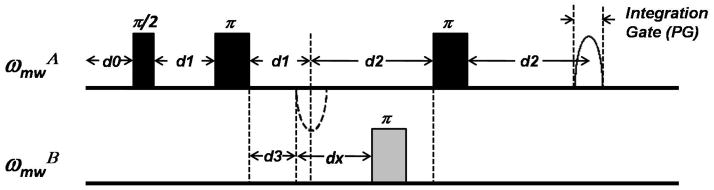
The four-pulse DEER sequence with the pulse spacings labeled according to Bruker Xepr software package nomenclature. In reference to the four-pulse DEER sequence in Figure 2, d1 = τ1 and d2 = τ2 (or τmax). The time increment parameter dx is calculated as d2/N, where N is the number of real data points. The start position of the echo signal is assigned as d0 while d3 is a critical delay parameter that prevents overlapping of the second observe pulse and pump pulse.
BASIC PROTOCOL 4: Analysis of DEER Data
For a complete understanding of how to properly analyze data from DEER experiments, the reader is directed to a number of excellent sources (Jeschke, 2002; Jeschke et al., 2004a; Chiang et al., 2005; Jeschke et al., 2006), including the DeerAnalysis2011 user’s manual (available online at www.epr.ethz.ch) for those wishing to analyze their data with this software. In this section, the process of converting a dipolar evolution curve into a distance profile will be outlined. The dipolar modulation curve is the manifestation of the additional modulation imposed upon A spins by their coupling with the B spins. The frequency of this additional modulation can be determined in a variety of ways.
The simplest method is to obtain the Fourier transform of the dipolar modulation curve so as to generate a Pake pattern in the frequency domain, where the splitting between the singularities is proportional to 1/r3, where r is the inter-spin distance (Figure 7, Method #1). Then, the Pake pattern needs to be simulated to obtain the distance profiles. A common approach to obtain distance profiles, particularly well-suited for noisy data sets, is the use of curve fitting to optimize the solution (Figure 7, Method #2). There are many variations of this method, but all include a modeling of the distance profile based on the current information on the system and generating the corresponding theoretical dipolar evolution curve for comparison with the experimental data. The process involves changing the distance profile to optimize the fit between the theoretical and experimental dipolar evolution curves. One variation of this approach utilizes Monte Carlo (MC) methods to generate a distance profile with an assumed form, such as Gaussian or Lorentzian shape, by combining random functions (Sen et al., 2007).
Figure 7.

Schematic diagram of three methods utilized for obtaining distance information from the background-subtracted dipolar evolution curve.
The third method, Tikhonov regularization (TKR) (Chiang et al., 2005), is a mathematical method used for solving an ill-posed problem by introducing a penalty for smoothness (Figure 7, Method #3). TKR uses the function in Equation 5,
| (Equation 5) |
to balance the quality of fit to the experimental data (first term) with the smoothness of the solution (second term) by varying the magnitude of the regularization parameter (α), where P is the probability distribution of the inter-spin distance, K is the operator that maps the function P onto the experimental data vector S, and L is usually a second derivative operator. The visual result of the TKR process is a plot of log η(α) against log ρ(α). Equations 6 and 7 give the corresponding equations used for plotting an L-curve.
| (Equation 6) |
| (Equation 7) |
Figure 8 illustrates the effect of non-optimal α values to the distance profile and the TKR fit. The distance profile in Figure 8 B is under-smoothed and corresponds to an α value that is too low. The corresponding dipolar evolution curve in Figure 8 C is over-fit such that the theoretical dipolar evolution curve was fit to some of the noise. The distance profile in Figure 8 D is qualitatively similar to the distance profile in B in that the most probable distance is within the breadth of the peak in D. However, the distance profile in D is smoother and corresponds to the optimal α value and dipolar evolution curve in Figure 8 E. The distance profile in Figure 8 F is over-smoothed and thus overly broad. The corresponding dipolar evolution curve in Figure 8 G is under fit, such that some of the oscillations in the signal are neglected in the TKR fit.
Figure 8.
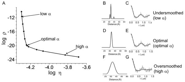
Example of an L-curve (A) and the corresponding distance profiles and dipolar modulation curves for low (B and C), optimal (D and E) and high (F and G) regularization parameters (α).
In the process of converting dipolar evolution curves to distance profiles (Figure 9), DeerAnalysis software uses a combination of shell factorization to simulate the dipolar evolution curves and Tikhonov regularization to optimize the solution. This software contains a variety of data analysis tools, such as approximate Pake transformation (APT), model fitting to a Gaussian or other user-defined functions, and options for background corrections.
Figure 9.
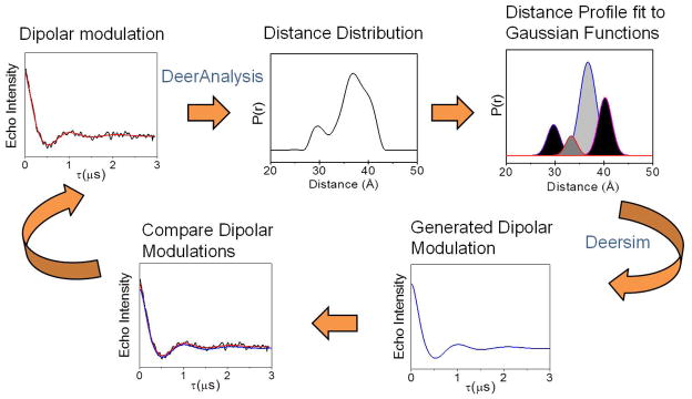
Self-consistent procedure for determining the appropriate level of background subtraction.
Materials
MatLab software
DeerAnalysis2011 software
DeerSim software (in-house software of the research group; available upon request)
-
Origin 8.5 software
Run DeerAnalysis2011 in MatLab environment.
Load the DEER spectrum in DeerAnalysis2011.
-
Select the appropriate zero time. Because the echo intensity data is set to start collecting before the top of the curve, the true zero time must be selected after data acquisition. A Gaussian function (Equation 8) can be fitted using a plotting software such as Origin 8.5 to data points from −300 to 300 ns. The center of the curve is assigned as the zero point.
(Equation 8) Data collected from 0 to τmax actually start at small negative time so that the data can be corrected for any discrepancy between the instrumental and actual zero time. -
Perform an initial background subtraction using an exponential function corresponding to a three-dimensional homogeneous background, and apply digital long pass filter to the dipolar evolution curve. Note that this is not necessarily the correct background subtraction level.
Digital long-pass filtering of the dipolar evolution curve prior to extraction of the distance profile can remove artifacts attributed to high-frequency noise and nuclear modulations (Jeschke et al., 2004a). -
Select Tikhonov regularization and generate the L-curve. Choose the distance distribution profile that corresponds to the regularization parameter situated at the corner of the L-curve (optimum α).
Note that a file that stores L-curve regularization parameters (α) could be altered so as to decrease α increments, which confers more resolution around the L-curve corner. This would enable more accurate determination of optimal α for longer distances and broader distance distribution profiles. -
Save this distance profile, then open DeerSim in MatLab.
Steps 6 – 8 are specific for our data analysis of HIV-1 protease distance profiles and are not followed by the entire EPR community. -
Regenerate the TKR distance profile using a linear combination of Gaussian-shaped functions with definite center positions, full width at half maxima (FWHM) and relative population percentages.
The initial guesses for these populations can be determined from software analysis such as those available in Origin8.5. -
Compare the Gaussian-regenerated dipolar modulation curve and the original echo curve with an initial background subtraction. If the two curves do not overlay, repeat steps 4 to 7 using a new background subtraction level for each attempt, until the two echo curves are perfectly overlaid. At this point, the level of background subtraction has been verified in a self-consistent manner and the distance profile has been deconstructed to the corresponding Gaussian populations (Figure 9).
For HIV-1 protease, these Gaussian populations correspond to various protein conformations that have been modeled by combining results from DEER, X-ray and molecular dynamic (MD) simulations. The meaning of the Gaussian populations will vary from system to system. The original use for the Gaussian reconstruction was a simple mathematical way to generate a theoretical echo curve in a MatLab environment for comparison to the TKR distance profile. This method was developed as a self-consistent method for background subtraction.
COMMENTARY
Background Information
Spin-labeling of Muscle Fibers
Early EPR studies focused on the role of the orientation and rotational motion of myosin heads in muscle contraction paved the way to spin-labeling studies of rabbitmuscle fibers. These experiments used spin labels with maleimide (MSL) and iodoacetamide (IASL) reactivities that target thiol groups on myosin heads (Thomas and Cooke, 1980; Thomas et al., 1980; Fajer et al., 1988; Fajer, 1994; Roopnarine and Thomas, 1994). Another study on rabbit skeletal muscles utilized the spin label 3-(5-fluoro-2,4-dinitroanilino)proxyl (FDNA) that is specific to the ε-amino group on a lysine residue in G-actin (Waring and Cooke, 1987). Spin-labeling conditions, such as pH, vary depending on the spin label used. For instance, labeling of thiol groups in myosin using MSL and IASL was done at pH 7.0 (Thomas and Cooke, 1980; Thomas et al., 1980; Fajer et al., 1988), while FDNA-labeling of lysine in G-actin was accomplished at a more basic condition (pH 8.0) (Waring and Cooke, 1987).
Synthetic and Orthogonal Labeling Strategies for Incorporating Unnatural Amino Acid Spin Labels
Aside from site-directed spin-labeling (SDSL), unnatural nitroxide amino acids, such as the conformationally constrained TOAC label can be added to specific sites of the protein during peptide synthesis (Hanson et al., 1998). Novel nitroxide labels can also be incorporated into the recombinant protein via the unique amber stop codon in an orthogonal labeling strategy (Cornish et al., 1994; Fleissner et al., 2009). These advances are important for consideration of protein systems where cysteine cannot be utilized as a labeling site, such as those that have functionally important native cysteine residues and disulfide bridges.
Critical Parameters and Troubleshooting
As illustrated in Figure 10, when considering only intramolecular distance, for F(t), the frequency and decay rate of the oscillations depend on the length of the most probable distance and the breadth of the distance distribution, respectively. By varying the breadth of a distance profile centered at 36 Å (Figure 10 A) from 1 to 10 Å and generating the theoretical dipolar evolution curves (Figure 10 B), it can be seen that the narrowest distributions have the most well-defined oscillations, corresponding to the longest decay rates. The frequency of oscillations can likewise be illustrated by comparing the dipolar evolution curves (Figure 10 D) corresponding to distance profiles (Figure 10 C) that have the same breadth (7 Å) and vary in the most probable distance from 18–78 Å. These dipolar evolution curves have different decay rates, but because the frequency of the oscillations also changes, the curves have the same number of oscillations before being completely damped. The inset in Figure 10 D highlights the dipolar evolution curves that decay within the first 2 μs, a common data acquisition parameter reported in literature. Curves with solid lines correspond to distances ≤ 36 Å. The dipolar evolution curves corresponding to center distances larger than 36 Å are plotted as dashed lines. The distinction is made to show which distances of this breadth have echo curves containing two full oscillations, which is required for accurate distance and distance breadth determination within 2 μs (Jeschke and Polyhach, 2007).
Figure 10.

Effect of the breadth and most probable distance on the dipolar modulation curves. (A) Varying FWHM of distance profiles centered at 36 Å and (B) the corresponding theoretical dipolar evolution curves with different decay rates; (C) Profiles with different center distances but same FWHM and (D) corresponding theoretical dipolar evolution curves with different oscillation frequencies. Inset highlights dipolar modulations that decay within the first 2 μs.
A practical consideration when setting up a DEER experiment is to properly choose the data acquisition time, τ2 or τmax, for the longest distance under consideration. Unfortunately, one of the difficulties with detecting longer distances with DEER is the increased pulse length time, where the overall signal intensity is dictated by the phase memory time, Tm, of the system. As τmax increases, the spacing between the Hahn echo pulses increases and the echo intensity decreases as dictated by spin-relaxation. Consequently, data acquisition time should be increased so as to attain the desired SNR. Data has been collected on protein samples for distances greater than 60 Å, however the acquisition times are typically long and SNR are lowered (Jeschke et al., 2004a; Jeschke and Polyhach, 2007; McHaourab et al., 2011). It is here where experiments performed at Q-band frequencies (Polyhach et al., 2012), as well as those using deuterated proteins or matrices (Ward et al., 2009; Ward et al., 2010), have an advantage.
Figure 11 demonstrates the effects of the chosen value of τmax on proper regeneration of the breadths of DEER distance distributions. A distance of 48 Å is chosen for this demonstration. Figure 11 A shows Gaussian-shaped distance distribution profiles centered at 48 Å with FWHM of 1 Å and 7Å. The theoretical dipolar evolution curves generated are shown in Figure 11 B. Given the theoretical echo curves do not contain any noise; we utilized the noise generator in Origin 8.0 to introduce white noise to a SNR of 40, a value that is typically twice of what we have obtained in HIV-1 protease experiments. The data sets were then truncated to τmax of 2 μs (Figure 11 C). We then utilized Tikhonov Regularization (TKR) methods in DeerAnalysis to generate distance profiles, which are shown in Figure 11 D. The most probable distance for the curves is the same (48.00 ± 0.01 Å), and the broader signal is accurately regenerated with a breadth of 7.0 ± 0.1Å. However, for τmax of 2 μs, the breadth of the 1 Å FWHM profile was broadened to 6.8 Å. If the echo curves are truncated to τmax values of 3–4 μs instead of 2 μs, the breath of the original distance distribution profiles are accurately regenerated. This exercise demonstrates that the accuracy of the breadth for the distance profile strongly relies on a sufficiently long τmax when collecting the dipolar evolution curve.
Figure 11.

The influence of τmax length to the corresponding distance profile. (A) Gaussian distance profiles with most probable distance of 48 Å with FWHM of 1 Å (solid) and 7 Å (dashed); (B) The corresponding theoretical dipolar evolution curves. Solid vertical line corresponds to τmax of 2 μs (C) The same dipolar evolution curves in (B) but τmax is shortened to 2 μs; (D) The corresponding TKR distance profiles for (C) analyzed using DeerAnalysis software.
To further illustrate the importance of collecting data at a sufficiently long τmax, Figure 12 A shows experimental dipolar evolution curves for Subtype B HIV-1 protease in deuterated matrix, collected as a function of τ or length of the dipolar evolution curve, and the corresponding distance profiles (Figure 12 B). These data were collected sequentially without sample thawing to ensure reproducibility of data acquisition. Dipolar evolution curves were analyzed with DeerAnalysis2008 in a manner such that the same background subtraction level was used. Data analysis reveals that the most probable distance is independent of τmax. However, a minor population centered at ~40 Å (vertical dashed line) appeared as a ‘shoulder’ that changes in intensity depending on the τmax used. Convergence of the shape of the distance profile resulted for τmax > 2.5 μs; suggesting that long acquisition times are necessary when information about the shape of the distance profile is required. When only the most probable distance is of interest, shorter values of τmax can be utilized, resulting in stronger signals and faster acquisition times.
Figure 12.
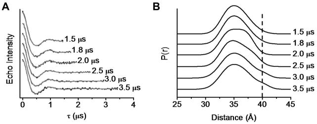
DEER data for Subtype B HIV-1 protease acquired at variable τmax. (A) Background-subtracted dipolar evolution curves and the corresponding TKR fits (gray solid line); (B) The corresponding TKR distance profiles. The vertical dashed line marks the position for a minor population centered at ~40 Å. Data are vertically offset for clarity.
In addition to choosing a long enough τ2, such as for long distance measurements or accurate distance profile shape, long acquisition times are also needed for proper background subtraction. Because the acquired signal, V(t), contains contributions from both the intramolecular signal F(t) and the background signal B(t), data needs to be collected for long enough times (τmax > τdecay) for accurate separation of B(t) from V(t). Typically, B(t) can be modeled by an exponential function of the form in Equation 9,
| (Equation 9) |
where D is the dimensionality of the background, typically three dimensions for soluble proteins and ln [B(t)] can be described as a simple low-order polynomial. If V(t) is collected such that τ2 is too short for the oscillations to be dampened, it becomes difficult to determine the proper background subtraction. Typically, when only a single distance, such as the most probable distance, is of interest, small errors in the background subtraction do not significantly alter the value of the derived most probable distance. However, when information from the shape of the distance profile or the presence of minor populations is desired, improper background subtraction can inadvertently affect the distance profiles obtained.
Note that the background subtraction for membrane protein samples can be troublesome. Given that the proteins are contained within the lipid leaflets of vesicles, which can be described as a 2D sheet, the 3D background may not be an appropriate model. Additionally, the concentration enhancement of integral proteins in lipid bilayers may completely abolish the oscillations in the raw data. To overcome this problem, novel membrane mimetic system of nanolipoprotein phospholipid bilayers, most commonly referred to as nanodiscs, have been pioneered and shown to be successful (Zou and McHaourab, 2010).
The distance limitations for DEER experiments are frequently cited as being from 15 Å to 60 Å or 80 Å. The lower limit arises from the requirement that the excitation bandwidth should exceed the electron-electron coupling which can be met only for distances ≥ 15 Å. The upper limit, on the other hand, is limited by the phase memory time (Tm), the inherent sensitivity of the system, sample concentration, and contribution from intermolecular interactions. For biological molecules, the solvent is typically restricted to aqueous solutions. Moreover, the biological molecule typically contains methyl protons, which contribute to shorter Tm. These restrictions typically limit the Tm to ≤ 5 μs, although 3–4 μs is more common. These Tm values set the time limit on the spacing between pulses, which corresponds to the evolution time in the echo curve. As shown above, this impacts one’s ability to accurately determine distances and breadths of distance profiles. In practice, Tm values of 3–4 μs correspond to the ability to measure distances of ≤ 60 Å, as a practical limit.
To increase the upper limit for distance measurements, Tm can be prolonged by deuteron replacement of protons in the sample. This can be done by replacing neighboring nuclei, usually from solvent and cryoprotectant with deuterium or by deuterating the protein (Ward et al., 2010). For instance, distance measurements up to 70 Å was achieved on the histone core particle by using deuterated solvents and 50% deuterated glycerol as glassing agent (Ward et al., 2009). Figure 13 shows the Tm curves in echo decay experiments for HIV-1 protease in protonated and deuterated matrices, revealing the dependence of Tm upon the solvent used. Tm is longest when the protein is in D2O and 30% deuterated glycerol, which enables longer distance measurements and improved signal-to-noise ratio of the corresponding dipolar modulation curves; hence faster data acquisition. Unfortunately, for buried spin-labels without access to the solvent, also the case for some membrane proteins, solvent deuteration does not always lead to an increase in Tm (Huber et al., 2001; Volkov et al., 2009).
Figure 13.

Intensity normalized Tm curves and corresponding exponential decay fits for MTSL-labeled HIV-1 protease in 2 mM NaOAc buffer pH 5.0 with H2O and 30% glycerol (dotted line), 2 mM NaOAc buffer pH 5.0 with H2O and 30% deuterated glycerol (dashed line), 2 mM NaOAc buffer pH 5.0 with D2O and 30% deuterated glycerol (solid line). The oscillations in the deuterated solvents originate from ESEEM effects between the deuterons and spin labels. The vertical dashed line marks τ = 3 μs.
Other methods to overcome limitations of Tm include alternative pulse sequences, such as variable time DEER (Jeschke et al., 2004a), 5-pulse DEER (Song et al., 2011) and six-pulse DQC ESR (Borbat et al., 2004). Although variable-time DEER confers increased sensitivity in most cases, it is not recommended for membrane proteins reconstituted in liposomes because of inhomogeneous spatial distribution in three dimensions and dominant instantaneous diffusion mechanism (Jeschke, 2012). Aside from variable time DEER, a 5-pulse version based on the 4-pulse DEER that provides longer acquisition time has been introduced. This sequence provides maximum suppression of spin diffusion and an extra pump pulse that allows up to twice as much dipolar evolution time and thus, longer distance measurement (Song et al., 2011). DQC, another pulsed EPR technique may also be employed. Partial suppression of the nuclear spin diffusion effects on electron spin Tm has been achieved using a six-pulse variant of DQC, also known as double quantum filtered refocused-electron spin echoes (DQFR-ESE), allowing accurate distance measurements up to ~70 Å (Borbat et al., 2004).
Attempts have also been made to measure longer distances by going to higher frequencies such as Q- and W-bands. The enhanced sensitivity observed at higher frequency stems from an increase in Boltzmann population difference between the spin states at the higher Zeeman energy, which contributes to signal improvement and increased sensitivity of the resonator at the higher frequency (Prisner et al., 2001). In addition, distance range increase for a membrane protein was reported at Q-band by employing discoidal nanoscale lipoprotein-bound bilayers (Zou and McHaourab, 2010). Meanwhile, utilization of Gd3+ markers took advantage of the higher spin quantum number for these nuclei, enabling distance measurements in the 60–100 Å range at Ka and W-band frequencies (Song et al., 2011). Also note that several model systems, such as rod-like shape-persistent rigid biradicals, allowed distance measurements from 50 to 75 Å (Jeschke et al., 2004a).
Before acquiring any DEER data, it is important to make sure that the protein samples are free of contaminants and that they are homogeneous, and properly spin-labeled. Given that non labeled protein contaminants do not directly affect the DEER signal, oftentimes these aspects of sample purity are overlooked. However, in cases where sample homogeneity is important, all steps must be taken to ensure sample quality. Typically, size exclusion chromatography and then an analytical high pressure liquid chromatography (HPLC) trace are suitable means to demonstrate a homogeneous protein sample. Moreover, the spin-labeled protein samples can be analyzed by electrospray ionization time-of-flight mass spectrometry (ESI-TOF-MS) to validate homogeneous spin labeling. If necessary, tandem mass spectrometry (MS-MS) methods can also be utilized to confirm the location of the spin label, such as HPLC-ESI-ion trap-MSn and matrix-assisted laser desorption ionization (MALDI) TOF tandem MS of the protein tryptic digest.
Results from TKR analysis often generate distance profiles that have more than one peak. Questions arise as to the significance of these smaller peaks. The Gaussian self-consistent method will oftentimes also regenerate these smaller signals. Depending on the signal-to-noise ratio of the raw dipolar modulation curve, minor peaks with relative population percentage <5% may or may not be real. These peaks may be omitted or suppressed when regenerating the dipolar evolution curve. If the model curve is statistically comparable to the experimental curve by χ2 analysis (Equation 10 and 11) (Gabrys et al., 2003; de Vera et al., 2012) then the suppressed population is an artifact at the confidence level used, usually set to 95%. In Equation 10, we assume that a data point in the TKR curve ( ) is the expected value ( ). The calculated model echo curve, which corresponds to one or more suppressed Gaussian populations, is represented by . The noise parameter, σy is given in Equation 11, where is a point in the echo curve, is a data point in the TKR fit, and n is the number of data points employed.
| (Equation 10) |
| (Equation 11) |
Anticipated Results
Figure 14 shows a sample DEER result for HIV-1 protease. The Tikhonov regularization (TKR) distance distribution profiles were obtained from the background-subtracted and long-pass filtered dipolar modulation curves using DeerAnalysis2011. The optimum regularization parameter, selected right at the corner of the L-curve, was used for TKR. Gaussian-shaped functions were then used to regenerate the TKR distance profile. Populations with relative percentage of ≤ 5% were validated by suppressing them individually and regenerating a dipolar modulation model (Blackburn et al., 2009; Kear et al., 2009; de Vera et al., 2012). If the model curve is comparable to the original dipolar evolution curve using the χ2 criteria, then the questionable minor populations are regarded as artifacts of noise (de Vera et al., 2012). The asterisks in Figure 14 E indicate that these two small peaks were determined to be insignificant at the 95% confidence level.
Figure 14.

DEER data processing for an HIV-1 protease sample. (A) Determination of zero time (xc) by fitting a Gaussian function to the −300 to 300 ns region of the echo curve. (B) Raw dipolar echo curve and the exponential decay function (red solid line) corresponding to a homogeneous three-dimensional distribution that is employed for background subtraction. (C) Long-pass filtered and background-subtracted dipolar modulation curve with Tikhonov regularization (TKR) fit (red solid line) overlaid with Gaussian-reconstructed dipolar modulation (blue solid line). (D) The L-curves derived from TKR analysis that helps determine the optimal regularization parameter (α). (E) TKR distance profile overlaid with the linear combination of Gaussian populations (red dashed line). Peaks labeled with asterisk indicate populations ≤ 5% that are not statistically significant at 95% confidence level based on the χ2 criterion. (F) The Gaussian populations employed to regenerate the TKR distance profile. (G) The Pake dipolar pattern that results from the Fourier transformation of the background-subtracted dipolar modulation curve and the corresponding fit (red dashed line). (H) Table of values for the most probable (center) distances, full width at half maxima (FWHM), and relative percentage of conformational populations (Pop. %) used for generating the Gaussian-reconstructed distance profile in E (red dashed line).
Time Considerations
Using this protocol, DEER data acquisition at 65 K via an X-band spectrometer, on average, takes 4 to 16 hours for a homogeneously spin-labeled sample and 2 days for a poorly-labeled sample. For longer distance measurements and narrower distance profiles, dipolar evolution time needs to be prolonged and acquisition time will increase. Note that the maximum dipolar evolution time (τmax) should be chosen by the anticipated distance and distance distribution profile, but its maximum value is limited by the phase memory time (Tm) of the sample. Thus, for longer distances, using a deuterated matrix or protein deuteration may be necessary for longer Tm and higher SNR. Data acquisition on higher field spectrometers significantly lowers the acquisition time and extends the possible concentration range for DEER investigations.
LITERATURE CITED
- Altenbach C, Kusnetzow AK, Ernst OP, Hofmann KP, Hubbell WL. High-resolution distance mapping in rhodopsin reveals the pattern of helix movement due to activation. Proc Natl Acad Sci U S A. 2008;105:7439–7444. doi: 10.1073/pnas.0802515105. [DOI] [PMC free article] [PubMed] [Google Scholar]
- Altenbach C, Oh KJ, Trabanino RJ, Hideg K, Hubbell WL. Estimation of inter-residue distances in spin labeled proteins at physiological temperatures: experimental strategies and practical limitations. Biochemistry. 2001;40:15471–15482. doi: 10.1021/bi011544w. [DOI] [PubMed] [Google Scholar]
- Bennati M, Weber A, Antonic J, Perlstein DL, Robblee J, Stubbe J. Pulsed ELDOR spectroscopy measures the distance between the two tyrosyl radicals in the R2 subunit of the E. coli ribonucleotide reductase. J Am Chem Soc. 2003;125:14988–14989. doi: 10.1021/ja0362095. [DOI] [PubMed] [Google Scholar]
- Berliner LJ, Eaton SS, Eaton GE. Distance Measurements in Biological Systems by EPR. Kluwer Academic/Plenum Publishers; New York: 2000. [Google Scholar]
- Blackburn ME, Veloro AM, Fanucci GE. Monitoring inhibitor-induced conformational population shifts in HIV-1 protease by pulsed EPR spectroscopy. Biochemistry. 2009;48:8765–8767. doi: 10.1021/bi901201q. [DOI] [PubMed] [Google Scholar]
- Borbat PP, Crepeau RH, Freed JH. Multifrequency two-dimensional Fourier transform ESR: an X/Ku-band spectrometer. J Magn Reson. 1997;127:155–167. doi: 10.1006/jmre.1997.1201. [DOI] [PubMed] [Google Scholar]
- Borbat PP, Davis JH, Butcher SE, Freed JH. Measurement of large distances in biomolecules using double-quantum filtered refocused electron spin-echoes. J Am Chem Soc. 2004;126:7746–7747. doi: 10.1021/ja049372o. [DOI] [PubMed] [Google Scholar]
- Borbat PP, Mchaourab H, Freed JH. Protein structure determination using long-distance constraints from double-quantum coherence ESR: Study of T4 Lysozyme. Biophysical Journal. 2002;82:360A–360A. doi: 10.1021/ja020040y. [DOI] [PubMed] [Google Scholar]
- Cai Q, Kusnetzow AK, Hideg K, Price EA, Haworth IS, Qin PZ. Nanometer distance measurements in RNA using site-directed spin labeling. Biophys J. 2007;93:2110–2117. doi: 10.1529/biophysj.107.109439. [DOI] [PMC free article] [PubMed] [Google Scholar]
- Chiang YW, Borbat PP, Freed JH. The determination of pair distance distributions by pulsed ESR using Tikhonov regularization. J Magn Reson. 2005;172:279–295. doi: 10.1016/j.jmr.2004.10.012. [DOI] [PubMed] [Google Scholar]
- Cooke JA, Brown LJ. Distance measurements by continuous wave EPR spectroscopy to monitor protein folding. Methods Mol Biol. 2011;752:73–96. doi: 10.1007/978-1-60327-223-0_6. [DOI] [PubMed] [Google Scholar]
- Cornish VW, Benson DR, Altenbach CA, Hideg K, Hubbell WL, Schultz PG. Site-specific incorporation of biophysical probes into proteins. Proc Natl Acad Sci U S A. 1994;91:2910–2914. doi: 10.1073/pnas.91.8.2910. [DOI] [PMC free article] [PubMed] [Google Scholar]
- Dastvan R, Bode BE, Karuppiah MP, Marko A, Lyubenova S, Schwalbe H, Prisner TF. Optimization of transversal relaxation of nitroxides for pulsed electron-electron double resonance spectroscopy in phospholipid membranes. J Phys Chem B. 2010;114:13507–13516. doi: 10.1021/jp1060039. [DOI] [PubMed] [Google Scholar]
- de Vera IMS, Blackburn ME, Fanucci GE. Correlating conformational shift induction with altered inhibitor potency in a multidrug resistant HIV-1 protease variant. Biochemistry. 2012 doi: 10.1021/bi301010z. [DOI] [PMC free article] [PubMed] [Google Scholar]
- Durrant JD, McCammon JA. Molecular dynamics simulations and drug discovery. BMC Biol. 2011;9:71. doi: 10.1186/1741-7007-9-71. [DOI] [PMC free article] [PubMed] [Google Scholar]
- Fajer P. Electron Spin Resonance Spectroscopy Labeling in Peptide and Protein Analysis. In: Meyers RA, editor. Encyclopedia of Analytical Chemistry. John Wiley and Sons, Ltd; 2000. pp. 5725–5761. [Google Scholar]
- Fajer P, Brown L, Song L. Practical Pulsed Dipolar ESR (DEER) Spin Labeling. 2006;1:95–128. [Google Scholar]
- Fajer PG. Determination of spin-label orientation within the myosin head. Proc Natl Acad Sci U S A. 1994;91:937–941. doi: 10.1073/pnas.91.3.937. [DOI] [PMC free article] [PubMed] [Google Scholar]
- Fajer PG, Fajer EA, Brunsvold NJ, Thomas DD. Effects of AMPPNP on the orientation and rotational dynamics of spin-labeled muscle cross-bridges. Biophys J. 1988;53:513–524. doi: 10.1016/S0006-3495(88)83131-X. [DOI] [PMC free article] [PubMed] [Google Scholar]
- Fanucci GE, Lee JY, Cafiso DS. Spectroscopic Evidence that Osmolytes in Crystallization Buffers Inhibit a Conformational Change in a Membrane Protein. Biochemistry. 2003;42:13106–13222. doi: 10.1021/bi035439t. [DOI] [PubMed] [Google Scholar]
- Fanucci GE, Cafiso DS. Recent advances and applications of site-directed spin labeling. Curr Opin Struct Biol. 2006;16:644–653. doi: 10.1016/j.sbi.2006.08.008. [DOI] [PubMed] [Google Scholar]
- Fawzi NL, Fleissner MR, Anthis NJ, Kalai T, Hideg K, Hubbell WL, Clore GM. A rigid disulfide-linked nitroxide side chain simplifies the quantitative analysis of PRE data. J Biomol NMR. 2011;51:105–114. doi: 10.1007/s10858-011-9545-x. [DOI] [PMC free article] [PubMed] [Google Scholar]
- Fleissner MR, Bridges MD, Brooks EK, Cascio D, Kalai T, Hideg K, Hubbell WL. Structure and dynamics of a conformationally constrained nitroxide side chain and applications in EPR spectroscopy. Proc Natl Acad Sci U S A. 2011;108:16241–16246. doi: 10.1073/pnas.1111420108. [DOI] [PMC free article] [PubMed] [Google Scholar]
- Fleissner MR, Brustad EM, Kalai T, Altenbach C, Cascio D, Peters FB, Hideg K, Peuker S, Schultz PG, Hubbell WL. Site-directed spin labeling of a genetically encoded unnatural amino acid. Proc Natl Acad Sci U S A. 2009;106:21637–21642. doi: 10.1073/pnas.0912009106. [DOI] [PMC free article] [PubMed] [Google Scholar]
- Gabrys CM, Yang J, Weliky DP. Analysis of local conformation of membrane-bound and polycrystalline peptides by two-dimensional slow-spinning rotor-synchronized MAS exchange spectroscopy. J Biomol NMR. 2003;26:49–68. doi: 10.1023/a:1023060102409. [DOI] [PubMed] [Google Scholar]
- Galiano L, Blackburn ME, Veloro AM, Bonora M, Fanucci GE. Solute effects on spin labels at an aqueous-exposed site in the flap region of HIV-1 protease. J Phys Chem B. 2009a;113:1673–1680. doi: 10.1021/jp8057788. [DOI] [PubMed] [Google Scholar]
- Galiano L, Ding F, Veloro AM, Blackburn ME, Simmerling C, Fanucci GE. Drug pressure selected mutations in HIV-1 protease alter flap conformations. J Am Chem Soc. 2009b;131:430–431. doi: 10.1021/ja807531v. [DOI] [PMC free article] [PubMed] [Google Scholar]
- Gekko K, Timasheff SN. Mechanism of protein stabilization by glycerol: preferential hydration in glycerol-water mixtures. Biochemistry. 1981;20:4667–4676. doi: 10.1021/bi00519a023. [DOI] [PubMed] [Google Scholar]
- Georgieva ER, Roy AS, Grigoryants VM, Borbat PP, Earle KA, Scholes CP, Freed JH. Effect of freezing conditions on distances and their distributions derived from Double Electron Electron Resonance (DEER): a study of doubly-spin-labeled T4 lysozyme. J Magn Reson. 2012;216:69–77. doi: 10.1016/j.jmr.2012.01.004. [DOI] [PMC free article] [PubMed] [Google Scholar]
- Getz EB, Xiao M, Chakrabarty T, Cooke R, Selvin PR. A comparison between the sulfhydryl reductants tris(2-carboxyethyl)phosphine and dithiothreitol for use in protein biochemistry. Anal Biochem. 1999;273:73–80. doi: 10.1006/abio.1999.4203. [DOI] [PubMed] [Google Scholar]
- Ghimire H, McCarrick RM, Budil DE, Lorigan GA. Significantly improved sensitivity of Q-band PELDOR/DEER experiments relative to X-band is observed in measuring the intercoil distance of a leucine zipper motif peptide (GCN4-LZ) Biochemistry. 2009;48:5782–5784. doi: 10.1021/bi900781u. [DOI] [PMC free article] [PubMed] [Google Scholar]
- Han JC, Han GY. A procedure for quantitative determination of tris(2-carboxyethyl)phosphine, an odorless reducing agent more stable and effective than dithiothreitol. Anal Biochem. 1994;220:5–10. doi: 10.1006/abio.1994.1290. [DOI] [PubMed] [Google Scholar]
- Hanson P, Anderson DJ, Martinez G, Millhauser G, Formaggio F, Crisma M, Toniolo C, Vita C. Electron spin resonance and structural analysis of water soluble, alanine-rich peptides incorporating TOAC. Molecular Physics. 1998;95:957–966. [Google Scholar]
- Hubbell WL, Gross A, Langen R, Lietzow MA. Recent advances in site-directed spin labeling of proteins. Curr Op Struct Biol. 1998;8:649–656. doi: 10.1016/s0959-440x(98)80158-9. [DOI] [PubMed] [Google Scholar]
- Huber M, Lindgren M, Hammarstrom P, Martensson LG, Carlsson U, Eaton GR, Eaton SS. Phase memory relaxation times of spin labels in human carbonic anhydrase II: pulsed EPR to determine spin label location. Biophysical Chemistry. 2001;94:245–256. doi: 10.1016/s0301-4622(01)00239-3. [DOI] [PubMed] [Google Scholar]
- Huyghues-Despointes BM, Pace CN, Englander SW, Scholtz JM. Measuring the conformational stability of a protein by hydrogen exchange. Methods Mol Biol. 2001;168:69–92. doi: 10.1385/1-59259-193-0:069. [DOI] [PubMed] [Google Scholar]
- Jeschke G. Distance measurements in the nanometer range by pulse EPR. Chemphyschem. 2002;3:927–932. doi: 10.1002/1439-7641(20021115)3:11<927::AID-CPHC927>3.0.CO;2-Q. [DOI] [PubMed] [Google Scholar]
- Jeschke G. DEER distance measurements on proteins. Annu Rev Phys Chem. 2012;63:419–446. doi: 10.1146/annurev-physchem-032511-143716. [DOI] [PubMed] [Google Scholar]
- Jeschke G, Bender A, Paulsen H, Zimmermann H, Godt A. Sensitivity enhancement in pulse EPR distance measurements. J Magn Reson. 2004a;169:1–12. doi: 10.1016/j.jmr.2004.03.024. [DOI] [PubMed] [Google Scholar]
- Jeschke G, Chechik V, Ionita P, Godt A, Zimmermann H, Banham J, Timmel CR, Hilger D, Jung H. DeerAnalysis2006 - A Comprehensive Software Package for Analyzing Pulsed ELDOR Data. Appl Mag Reson. 2006;30:473–498. [Google Scholar]
- Jeschke G, Panek G, Godt A, Bender A, Paulsen H. Data analysis procedures for pulse ELDOR measurements of broad distance distributions. Applied Magnetic Resonance. 2004b;26:223–244. [Google Scholar]
- Jeschke G, Polyhach Y. Distance measurements on spin-labelled biomacromolecules by pulsed electron paramagnetic resonance. Physical Chemistry Chemical Physics. 2007;9:1895–1910. doi: 10.1039/b614920k. [DOI] [PubMed] [Google Scholar]
- Jeschke G, Wegener C, Nietschke M, Jung H, Steinhoff HJ. Interresidual distance determination by four-pulse double electron-electron resonance in an integral membrane protein: the Na+/proline transporter PutP of Escherichia coli. Biophys J. 2004c;86:2551–2557. doi: 10.1016/S0006-3495(04)74310-6. [DOI] [PMC free article] [PubMed] [Google Scholar]
- Kear JL, Blackburn ME, Veloro AM, Dunn BM, Fanucci GE. Subtype polymorphisms among HIV-1 protease variants confer altered flap conformations and flexibility. J Am Chem Soc. 2009;131:14650–14651. doi: 10.1021/ja907088a. [DOI] [PMC free article] [PubMed] [Google Scholar]
- Kim M, Xu Q, Fanucci GE, Cafiso DS. Solutes modify a conformational transition in a membrane transport protein. Biophys J. 2006;90:2922–2929. doi: 10.1529/biophysj.105.078246. [DOI] [PMC free article] [PubMed] [Google Scholar]
- Kim NK, Bowman MK, DeRose VJ. Precise mapping of RNA tertiary structure via nanometer distance measurements with double electron-electron resonance spectroscopy. J Am Chem Soc. 2010;132:8882–8884. doi: 10.1021/ja101317g. [DOI] [PMC free article] [PubMed] [Google Scholar]
- Kuttner YY, Kozer N, Segal E, Schreiber G, Haran G. Separating the contribution of translational and rotational diffusion to protein association. J Am Chem Soc. 2005;127:15138–15144. doi: 10.1021/ja053681c. [DOI] [PubMed] [Google Scholar]
- Lavalette D, Hink MA, Tourbez M, Tetreau C, Visser AJ. Proteins as micro viscosimeters: Brownian motion revisited. Eur Biophys J. 2006;35:517–522. doi: 10.1007/s00249-006-0060-z. [DOI] [PubMed] [Google Scholar]
- Lee JC, Timasheff SN. The stabilization of proteins by sucrose. J Biol Chem. 1981;256:7193–7201. [PubMed] [Google Scholar]
- López CJ, Fleissner MR, Guo Z, Kismetzpw AK, Hubbell WL. Osmolyte perturbation reveals conformational equilibria in spin-labeled proteins. Prot Science. 2009;18:1637–1652. doi: 10.1002/pro.180. [DOI] [PMC free article] [PubMed] [Google Scholar]
- Lovett JE, Bowen AM, Timmel CR, Jones MW, Dilworth JR, Caprotti D, Bell SG, Wong LL, Harmer J. Structural information from orientationally selective DEER spectroscopy. Phys Chem Chem Phys. 2009;11:6840–6848. doi: 10.1039/b907010a. [DOI] [PubMed] [Google Scholar]
- Mao Q, Schleidt S, Zimmermann H, Jeschke G. A pulsed EPR study of surfactant layer structure in composites of a synthetic layered silicate with polystyrene and polycaprolactone. Phys Chem Chem Phys. 2008;10:1156–1167. doi: 10.1039/b713788e. [DOI] [PubMed] [Google Scholar]
- McHaourab HS, Oh KJ, Fang CJ, Hubbell WL. Conformation of T4 lysozyme in solution. Hinge-bending motion and the substrate-induced conformational transition studied by site-directed spin labeling. Biochemistry. 1997;36:307–316. doi: 10.1021/bi962114m. [DOI] [PubMed] [Google Scholar]
- McHaourab HS, Steed PR, Kazmier K. Toward the fourth dimension of membrane protein structure: insight into dynamics from spin-labeling EPR spectroscopy. Structure. 2011;19:1549–1561. doi: 10.1016/j.str.2011.10.009. [DOI] [PMC free article] [PubMed] [Google Scholar]
- Miick SM, Martinez GV, Fiori WR, Todd AP, Millhauser GL. Short alanine-based peptides may form 3(10)-helices and not alpha-helices in aqueous solution. Nature. 1992;359:653–655. doi: 10.1038/359653a0. [DOI] [PubMed] [Google Scholar]
- Milov AD, Maryasov AG, Tsvetkov YD, Raap J. Pulsed ELDOR in spin-labeled polypeptides. Chemical Physics Letters. 1999;303:135–143. [Google Scholar]
- Misra SK, Borbat PP, Freed JH. Calculation of Double-Quantum-Coherence Two-dimensional Spectra: Distance Measurements and Orientational Correlations. Appl Magn Reson. 2009;36:237–258. doi: 10.1007/s00723-009-0023-5. [DOI] [PMC free article] [PubMed] [Google Scholar]
- Narr E, Godt A, Jeschke G. Selective measurements of a nitroxide-nitroxide separation of 5 nm and a nitroxide-copper separation of 2.5 nm in a terpyridine-based copper(II) complex by pulse EPR spectroscopy. Angew Chem Int Ed Engl. 2002;41:3907–3910. doi: 10.1002/1521-3773(20021018)41:20<3907::AID-ANIE3907>3.0.CO;2-T. [DOI] [PubMed] [Google Scholar]
- Pannier M, Veit S, Godt A, Jeschke G, Spiess HW. Dead-time free measurement of dipole-dipole interactions between electron spins. J Magn Reson. 2000;142:331–340. doi: 10.1006/jmre.1999.1944. [DOI] [PubMed] [Google Scholar]
- Persson M, Harbridge JR, Hammarstrom P, Mitri R, Martensson LG, Carlsson U, Eaton GR, Eaton SS. Comparison of electron paramagnetic resonance methods to determine distances between spin labels on human carbonic anhydrase II. Biophys J. 2001;80:2886–2897. doi: 10.1016/S0006-3495(01)76254-6. [DOI] [PMC free article] [PubMed] [Google Scholar]
- Pistolesi S, Pogni R, Feix JB. Membrane insertion and bilayer perturbation by antimicrobial peptide CM15. Biophys J. 2007;93:1651–1660. doi: 10.1529/biophysj.107.104034. [DOI] [PMC free article] [PubMed] [Google Scholar]
- Polyhach Y, Bordignon E, Jeschke G. Rotamer libraries of spin labelled cysteines for protein studies. Physical Chemistry Chemical Physics. 2011;13:2356–2366. doi: 10.1039/c0cp01865a. [DOI] [PubMed] [Google Scholar]
- Polyhach Y, Bordignon E, Tschaggelar R, Gandra S, Godt A, Jeschke G. High sensitivity and versatility of the DEER experiment on nitroxide radical pairs at Q-band frequencies. Phys Chem Chem Phys. 2012 doi: 10.1039/c2cp41520h. [DOI] [PubMed] [Google Scholar]
- Polyhach Y, Jeschke G. Prediction of favourable sites for spin labelling of proteins. Spectroscopy-an International Journal. 2010;24:651–659. [Google Scholar]
- Potapov A, Yagi H, Huber T, Jergic S, Dixon NE, Otting G, Goldfarb D. Nanometer-scale distance measurements in proteins using Gd3+ spin labeling. J Am Chem Soc. 2010;132:9040–9048. doi: 10.1021/ja1015662. [DOI] [PubMed] [Google Scholar]
- Prisner T, Rohrer M, MacMillan F. Pulsed EPR spectroscopy: biological applications. Annu Rev Phys Chem. 2001;52:279–313. doi: 10.1146/annurev.physchem.52.1.279. [DOI] [PubMed] [Google Scholar]
- Rabenstein MD, Shin YK. Determination of the distance between two spin labels attached to a macromolecule. Proc Natl Acad Sci U S A. 1995;92:8239–8243. doi: 10.1073/pnas.92.18.8239. [DOI] [PMC free article] [PubMed] [Google Scholar]
- Raitsimring AM, Gunanathan C, Potapov A, Efremenko I, Martin JM, Milstein D, Goldfarb D. Gd3+ complexes as potential spin labels for high field pulsed EPR distance measurements. J Am Chem Soc. 2007;129:14138–14139. doi: 10.1021/ja075544g. [DOI] [PubMed] [Google Scholar]
- Riplinger C, Kao JP, Rosen GM, Kathirvelu V, Eaton GR, Eaton SS, Kutateladze A, Neese F. Interaction of radical pairs through-bond and through-space: scope and limitations of the point-dipole approximation in electron paramagnetic resonance spectroscopy. J Am Chem Soc. 2009;131:10092–10106. doi: 10.1021/ja901150j. [DOI] [PMC free article] [PubMed] [Google Scholar]
- Roessler MM, King MS, Robinson AJ, Armstrong FA, Harmer J, Hirst J. Direct assignment of EPR spectra to structurally defined iron-sulfur clusters in complex I by double electron-electron resonance. Proc Natl Acad Sci U S A. 2010;107:1930–1935. doi: 10.1073/pnas.0908050107. [DOI] [PMC free article] [PubMed] [Google Scholar]
- Roopnarine O, Thomas DD. A spin label that binds to myosin heads in muscle fibers with its principal axis parallel to the fiber axis. Biophys J. 1994;67:1634–1645. doi: 10.1016/S0006-3495(94)80636-8. [DOI] [PMC free article] [PubMed] [Google Scholar]
- Schiemann O, Cekan P, Margraf D, Prisner TF, Sigurdsson ST. Relative Orientation of Rigid Nitroxides by PELDOR: Beyond Distance Measurements in Nucleic Acids. Angewandte Chemie-International Edition. 2009;48:3292–3295. doi: 10.1002/anie.200805152. [DOI] [PubMed] [Google Scholar]
- Schreier S, Bozelli JC, Jr, Marin N, Vieira RF, Nakaie CR. The spin label amino acid TOAC and its uses in studies of peptides: chemical, physicochemical, spectroscopic, and conformational aspects. Biophys Rev. 2012;4:45–66. doi: 10.1007/s12551-011-0064-5. [DOI] [PMC free article] [PubMed] [Google Scholar]
- Sen KI, Logan TM, Fajer PG. Protein dynamics and monomer-monomer interactions in AntR activation by electron paramagnetic resonance and double electron-electron resonance. Biochemistry. 2007;46:11639–11649. doi: 10.1021/bi700859p. [DOI] [PubMed] [Google Scholar]
- Song Y, Meade TJ, Astashkin AV, Klein EL, Enemark JH, Raitsimring A. Pulsed dipolar spectroscopy distance measurements in biomacromolecules labeled with Gd(III) markers. J Magn Reson. 2011;210:59–68. doi: 10.1016/j.jmr.2011.02.010. [DOI] [PMC free article] [PubMed] [Google Scholar]
- Suarez J, Ranguelova K, Jarzecki AA, Manzerova J, Krymov V, Zhao X, Yu S, Metlitsky L, Gerfen GJ, Magliozzo RS. An oxyferrous heme/protein-based radical intermediate is catalytically competent in the catalase reaction of Mycobacterium tuberculosis catalase-peroxidase (KatG) J Biol Chem. 2009;284:7017–7029. doi: 10.1074/jbc.M808106200. [DOI] [PMC free article] [PubMed] [Google Scholar]
- Thomas DD, Cooke R. Orientation of spin-labeled myosin heads in glycerinated muscle fibers. Biophys J. 1980;32:891–906. doi: 10.1016/S0006-3495(80)85024-7. [DOI] [PMC free article] [PubMed] [Google Scholar]
- Thomas DD, Ishiwata S, Seidel JC, Gergely J. Submillisecond rotational dynamics of spin-labeled myosin heads in myofibrils. Biophys J. 1980;32:873–889. doi: 10.1016/S0006-3495(80)85023-5. [DOI] [PMC free article] [PubMed] [Google Scholar]
- Timasheff SN. Protein hydration, thermodynamic binding, and preferential hydration. Biochemistry. 2002;41:13473–13482. doi: 10.1021/bi020316e. [DOI] [PubMed] [Google Scholar]
- Tsvetkov YD, Grishin YA. Techniques for EPR Spectroscopy of Pulsed Electron Double Resonance (PELDOR): A Review. Instruments and Experimental Techniques. 2009;52:615–636. [Google Scholar]
- Volkov A, Dockter C, Bund T, Paulsen H, Jeschke G. Pulsed EPR determination of water accessibility to spin-labeled amino acid residues in LHCIIb. Biophys J. 2009;96:1124–1141. doi: 10.1016/j.bpj.2008.09.047. [DOI] [PMC free article] [PubMed] [Google Scholar]
- Ward R, Bowman A, El-Mkami H, Owen-Hughes T, Norman DG. Long distance PELDOR measurements on the histone core particle. J Am Chem Soc. 2009;131:1348–1349. doi: 10.1021/ja807918f. [DOI] [PMC free article] [PubMed] [Google Scholar]
- Ward R, Bowman A, Sozudogru E, El-Mkami H, Owen-Hughes T, Norman DG. EPR distance measurements in deuterated proteins. J Magn Reson. 2010;207:164–167. doi: 10.1016/j.jmr.2010.08.002. [DOI] [PMC free article] [PubMed] [Google Scholar]
- Waring AJ, Cooke R. The molecular dynamics of actin measured by a spin probe attached to lysine. Arch Biochem Biophys. 1987;252:197–205. doi: 10.1016/0003-9861(87)90024-5. [DOI] [PubMed] [Google Scholar]
- Yang Z, Becker J, Saxena S. On Cu(II)-Cu(II) distance measurements using pulsed electron electron double resonance. J Magn Reson. 2007;188:337–343. doi: 10.1016/j.jmr.2007.08.006. [DOI] [PubMed] [Google Scholar]
- Yang Z, Kise D, Saxena S. An approach towards the measurement of nanometer range distances based on Cu2+ ions and ESR. J Phys Chem B. 2010;114:6165–6174. doi: 10.1021/jp911637s. [DOI] [PubMed] [Google Scholar]
- Yang Z, Liu Y, Borbat P, Zweier JL, Freed JH, Hubbell WL. Pulsed ESR Dipolar Spectroscopy for Distance Measurements in Immobilized Spin Labeled Proteins in Liquid Solution. J Am Chem Soc. 2012;134:9950–9952. doi: 10.1021/ja303791p. [DOI] [PMC free article] [PubMed] [Google Scholar]
- Zou P, McHaourab HS. Increased sensitivity and extended range of distance measurements in spin-labeled membrane proteins: Q-band double electron-electron resonance and nanoscale bilayers. Biophys J. 2010;98:L18–20. doi: 10.1016/j.bpj.2009.12.4193. [DOI] [PMC free article] [PubMed] [Google Scholar]