

Abstract
One of the major challenges in protein tertiary structure prediction is structure quality assessment. In many cases, protein structure prediction tools generate good structural models, but fail to select the best models from a huge number of candidates as the final output. In this study, we developed a sampling-based machine-learning method to rank protein structural models by integrating multiple scores and features. First, features such as predicted secondary structure, solvent accessibility and residue-residue contact information are integrated by two Radial Basis Function (RBF) models trained from different datasets. Then, the two RBF scores and five selected scoring functions developed by others, i.e., Opus-CA, Opus-PSP, DFIRE, RAPDF, and Cheng Score are synthesized by a sampling method. At last, another integrated RBF model ranks the structural models according to the features of sampling distribution. We tested the proposed method by using two different datasets, including the CASP server prediction models of all CASP8 targets and a set of models generated by our in-house software MUFOLD. The test result shows that our method outperforms any individual scoring function on both best model selection, and overall correlation between the predicted ranking and the actual ranking of structural quality.
INTRODUCTION
Protein tertiary structure is essential for understanding protein function [1]. The experimental approaches for determining protein structures, such as X-ray crystallography, nuclear magnetic resonance spectroscopy, are typically expensive and time-consuming, which cannot be used to solve most of the proteins characterized in high-throughput genome sequencing [2]. Compared to experimental approaches, computational methods are much cheaper and faster. As significant progress has been made over the past two decades [1, 3–6], computational methods are becoming more and more important for studying protein structures in recent years [7]. For protein structure prediction, most methods generate a large number of candidate models and only select a handful of structures, e.g., top one or top five models as final predictions. In many cases, good models were generated but the tools failed to select best models from the candidate model pool. This becomes a bottleneck in protein structure prediction, and hence ranking the predicted structural models is a very important research problem in structural bioinformatics [8].
Currently, approaches for ranking structural models can be basically classified into four categories: (1) physical-based energies, (2) knowledge-based scoring functions, (3) consensus approaches, and (4) machine learning-based scores. A physical-based energy calculates energy of a protein structural model, together with its interaction with the solvent according to some physical laws [9–10]. Physical-based energy is often time-consuming to compute and very sensitive to small atomic displacement. Hence, it is usually not directly applied in ranking structural models. A knowledge-based scoring function is extracted from the statistical distribution of atoms or residues, either their environments or interactions, in known native structures [11]. Many of knowledge-based scoring functions are useful in general [12–16]. However, knowledge-based scoring functions only reflect some averages of the statistical properties, which also have associated noises. As a result, the discerning power of knowledge-based scoring functions may be limited and its performance may vary substantially among different types of structural models. The idea of consensus approaches is that near-native structures have low free energy and thus tend to be most populated with similar conformations. This is often implemented by using representatives from the largest clusters in a model pool as the top candidates. Such an approach has been extended to CASP predictions [17–19], For example, it is reported that the consensus approaches select structures with the highest similarity scores to all the others (or a subset of references) in the pool as the best models [18–19]. Consensus methods perform very well when most of the models in the pool are close to the native structure or at least not too far away from the native structure. However, when the model pool is dominated by poor models, it may perform worse than other knowledge-based approaches. Machine-learning methods assess model quality according to some trained “machines” [20–22], typically support vector machine or artificial neural networks using a set of structural models and their native structures. For example, a support vector regression model was proposed to take some abstracted structural features, including secondary structure and contact map features as input [22].
As demonstrated in CASP, consensus approaches typically work better than any individual knowledge-based scoring function in ranking structural models [23]. A reason behind the success of the consensus-based approach is that each individual tool captures some instead of all aspects of the native protein structure, and the correct prediction tends to be over-represented in a consensus model [24]. Machine learning-based scores using consensus-based features and features from individual structures extracted from a CASP training data set can further improve the performance [20]. The strength of machine-learning approach is its ability to “learn” the intrinsic rules from the differences between structural models and their native structures by combining various features that depict the models from different facets. The features might include structural features, features reflecting physical energy terms, knowledge-based scoring functions, as well as some comparisons between the features of a structural model and the predicted features from its amino acid sequence. However, consensus methods and machine learning methods using consensus information work very well in CASP only because there were so many tools to generate a large number of good and diverse models. Unfortunately, one typically cannot run many tools to obtain a suitable model pool in routing predictions for practical purposes. At the protein alignment level, some effort has been made to combine various energy terms using a consensus approach. A recent work [25] conducted threading for protein structure prediction by sampling weights of different potentials and applied an artificial neural network for target-specific weighting factor optimization. However, this method aimed to predict sequence-structure alignment in threading and could not be applied to quality assessment directly. By learning the spirit of consensus approaches and machine learning methods, we can apply a sampling scheme in a machine-learning frame to mimic their strengths without using many prediction tools. This is the rationale of this study and we believe the work will bring substantial benefit to individual structure prediction tool.
More specially, our sampling-based machine-learning method to rank structural models combines different existing knowledge-based scoring functions by a sampling method, and then uses radial basis function (RBF) neural networks to learn knowledge from the sampling distribution. In this way, the advantages of knowledge-based scoring functions, consensus approaches and machine learning-based scores can be combined. Our approach has two major contributions: (1) we integrate different features and scores systematically to obtain more discerning power for model quality assessment (QA); (2) we apply a sampling scheme and use sampling distribution features as input for more robust model QA.
In our method, five popular protein structural QA scores, as well as two of our machine-learning scores are adopted. The five existing scores are Opus-CA [13], Opus-PSP [14], DFIRE [15], RAPDF [16], and Cheng Score [22]. Taking multiple abstracted features of structural models as inputs, including secondary structures, solvent accessibilities and contact information, we construct an RBF model to predict model’s GDT_TS score. Although there are many metrics to measure the similarity of a model to its native structure, among of them the global distance test total score (GDT_TS) [26] is the most popular one, which has been typically applied in CASP. In this paper, we use GDT_TS also as a standard for structural QA. We have trained two RBF models to obtain two machine-learning scores. Furthermore, the two machine-learning scores and five existing scores are synthesized by a novel sampling process, which mimics consensus approaches. At last, we constructed an “integrated RBF model” as the “final machine”, which takes some sampling distribution features as inputs. Hence, we obtained a more robust score for model ranking from the integrated RBF model than that from each of individual scoring functions.
We have applied our method to two different datasets: one set is the CASP server prediction models of CASP8 targets, downloaded from http://www.predictioncenter.org/casp8/index.cgi, and the other set includes the models generated by our in-house software MUFOLD [27]. The test results show that our method performs significantly better than each individual approach on both selection of top models and Spearman Correlation between the predicted GDT_TS scores and the actual GDT_TS scores of the models to their native structures.
METHODS
Framework of the Approach
The overview of our method is presented in Fig. (1), which includes three main parts: (1) generating features and individual scores, (2) sampling process, and (3) integrating the RBF model. In part 1, we calculate five existing QA scores and two RBF scores for each model. In part 2, we apply a sampling process to simulate consensus methods. For this purpose, all the five existing scores and two RBF scores are normalized into z-scores [28]. Then a large number of weight sets are sampled to combine the seven z-scores into a set of new scores. In part 3, we study the distribution of the new scores, and retrieve several distribution features to build an integrated RBF model. Finally, we apply the score calculated by the integrated RBF to estimate the quality of each model.
Fig. 1.

Flowchart of the sampling-based approach.
Five QA Scores
We have done extensive survey and tests on existing QA scores. We finally selected five scoring functions, i.e., Opus-CA, Opus-PSP, DFIRE, RAPDF, and Cheng Score as features in this study. These scores are user-friendly and have better performance than other candidate scores that we evaluated on our testing datasets.
Opus-CA [13] is a knowledge-based potential function, which considers various molecular interactions, such as distance-dependent pair-wise energy with orientation preference, hydrogen bonding energy, short-range energy, packing energy, tri-peptide packing energy, three-body energy, and solvation energy. Opus-PSP [14] is a new version of Opus score, which also considers side-chain packing. DFIRE [15] includes a distance-scaled, finite ideal-gas reference (DFIRE) state to describe a residue specific, all-atom potential of mean force from a native protein structure database. RAPDF [16] uses three discriminatory functions to compute the probability of a structural model being native-like according to the set of pair-wise atom-atom distances. Cheng Score [22] applies a support vector regression method to assess the quality of a structural model by comparing the secondary structure, relative solvent accessibility, contact map, and beta-sheet structure of the model with the corresponding properties predicted from its primary sequence.
Abstracted Features for RBF
To evaluate the predicted protein structure models, two types of input features are generated for the learning “machines”. The first type of features is secondary structure based, which are abstracted from the comparison between the secondary structures (SS) / solvent accessibilities (SA) calculated from 3D coordinates of a model and those predicted from protein amino acid sequence. Here, the SS and SA of the model are calculated by DSSP [29], the predicted SS for the target sequence comes from PSIPRED [30], and the predicted SA for the target comes from SPINE [31]. Suppose the length of the target protein sequence is N, and the sequence is
| (1) |
where resi is the i-th residue of the sequence. Denote the calculated SS and SA of a model by DSSP as
| (2) |
| (3) |
where SSDi is the secondary structure of the i-th residue of the model and SSDi∈{α, β, c}≡{ss1, ss2, ss3}, which represents α-helix, β-sheet and coil, respectively, SADi ∈[0, 1] is the solvent accessibility of the i-th residue of the model. Denote the predicted SS and SA from the target sequence by PSIPred and SPINE as
| (4) |
| (5) |
where SSTij is the predicted probability of the secondary structure of the i-th residue being taken as ssj and SATi ∈[0, 1] is the predicted solvent accessibility of the i-th residue. By comparing the above two secondary structures, we obtain three features as follows:
| (6) |
where nj is the number of residues that satisfy SSDi = ssj (i = 1, 2, …, N).
To compare the above two solvent accessibilities, the 20 amino acids are divided into 3 categories with respect to their water solubility: (1) non-polar amino acids; (2) polar, neural amino acids; and (3) polar, charged amino acids. The non-polar amino acid set is denoted as R1 = {A, V, L, I, M, F, G, W, P}, the polar, neural amino acid set as R2 = {S, T, C, N, Q, Y}, and the polar, charged amino acid set as R3 = {K, R, H, D, E}, respectively. Then, three features are abstracted based on solvent accessibility:
| (7) |
where mk is the number of amino acids that satisfy aap ∈ Rk and aap is the p-th type of amino acid (p=1, 2, …, 20).
The second type of features is statistic based. We count the contact preferences of each type of amino acid within a given threshold distance. In a protein tertiary structure, we denote cpq(dis) as the contact number between the p-th type of amino acid aap and the q-th type of amino acid aaq (p, q=1, 2, …, 20) within the distance dis. For each distance threshold dis, we can get a 20-dimensional vector representing the “contact ability” of each type of amino acid (see Eq. 8) and a 210-dimensional vector that shows how likely two types of amino acids might interact with each other (see Eq. 9). The formula to calculate these two vectors are depicted as follows:
| (8) |
| (9) |
where ContactNum(dis) is the total number of contacts in the structure within distance threshold dis. We select 1400 native protein structures in PDB with homology less than 30% to obtain the averages of the above two vectors. We then calculate the Euclidian Distance and cosine value between each vector obtained in a predicted structural model and the same vector obtained from the native structure pool. We take two distance thresholds, namely 6Å and 12Å. Therefore, for each vector we get four features as the inputs of RBF.
RBF NNs
RBF is a variant of artificial neural networks and it has excellent nonlinear approximation properties [32]. A typically RBF network has three layers: input layer, hidden layer and output layer Fig. (2). An input vector X is used as input to RBF and the output of the network is a linear combination of the outputs from radial basis functions. Thus, the output y is computed as follows:
| (10) |
where Nh is the node number of hidden layer, Ci is the center of the i-th hidden node, and wi is the weight linking the i-th hidden node to the output node, respectively. A typical radial function is a Gaussian function:
| (11) |
where σ is the width of Gaussian function. By integrating Eq. (10) and Eq. (11), we can get
Fig. 2.

Architecture of a radial basis function (RBF) network
| (12) |
There are three types of parameters to be determined in RBF networks, the centers of hidden nodes, the widths of Gaussian functions, and the weights linking the hidden layer and output layer. In this study, all the parameters were trained by the steepest descent method.
We selected two different training data sets to train two RBF models. The first training data set is composed of randomly selected models of 32 CASP8 targets produced by MUFOLD. After discarding those models with quality lower than average in the first data set, we obtained the second dataset. The objective function of the training is the GDT_TS score of a model. In our study, the number of input nodes is 14 corresponding to the number of abstracted features and the number of hidden nodes is 35. The training is terminated after reaching 3000 cycles. The two RBF scores are integrated in the sampling process (described in the following section), together with the above five existing scoring functions.
Sampling Process for Integral RBF Model
After we get the above described five existing QA scores and two RBF scores, a sampling process is performed to integrate these seven scores. Our main idea is to generate a large number of “new scores”, which inherit the properties of selected individual QA scores, and hence, the distribution of the new scores will give us more discerning power with more robustness. For equal utilization of the seven scoring functions, each score is normalized by z-score [28] for all the models of a same protein target, which is defined by
| (13) |
where
| (14) |
| (15) |
Here, X is the score vector and xi represents the score of the i-th structural model in the pool.
A large number of weight sets are generated randomly to combine the above seven z-scores. Denote the k-th weight set as weightk = {Ωki}, k=1, 2,…,K, i =1, 2, …, 7, Ωki ∈ [0, 1] with a uniform random distribution, K is number of samples, taken as 1000 in our study, and i is an arbitrary order of individual scoring functions. As a result, a new sampling score is obtained according to the k-th weight set:
| (16) |
Then, we get K ranks for the each model according to K sampling scores.
After retrieving the distribution information of the sampling ranks, we found that the distribution features were well defined and robust. For example, we show the distributions of the sampling ranks of two structural models in Fig. (3), one is for CASP8 target 0388 with 174 residues in Fig. (3a) and the other is for CASP 8 target 0428 with 267 residues in Fig. (3b). From the data in Fig. (3), we can observe that both of them have relatively well-defined peaks but with different sharpness. For example, the peak in Fig. (3a) is very sharp and the center is around 18. In fact, the actual rank of this model in terms of its closeness to the native structure is 25 in a pool of 3000 candidate models and its GDT_TS against the native structure is 0.864. The number of 18 is very close to the actual rank of 25. While in Fig. (3b), the peak is wider and the center is around 335, which is also not far from its actual rank of 366 in 3000 models with a GDT of 0.818.
Fig. 3.
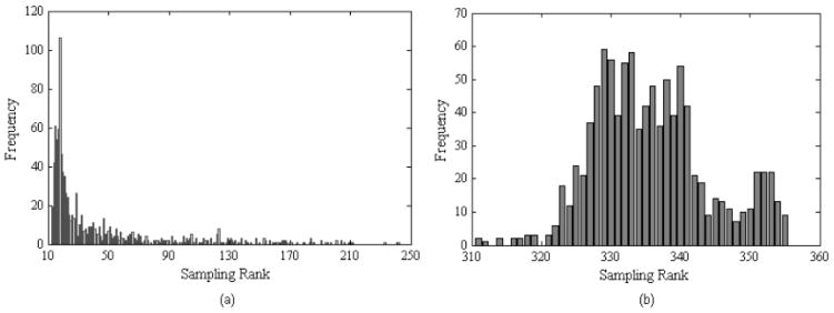
The sampling distributions of two structural models. (a) A model for CASP8 target 0388; (b) a model for CASP8 target 0428.
We abstract some distribution features, including the highest rank, the upper quartile rank, the median rank, the lower quartile rank, and the lowest rank of the distribution as the inputs of the integrated RBF model to retrieve actual rank information. In addition, we use two more features, i.e., ftop, the maximum frequency, i.e., the highest occurrence of any rank or the peak value in the distributions as shown in Fig. (3), and rtop, the rank associated with ftop. All these features are normalized by the total sample size before we input them in the RBF model.
Fig. (4) shows sampling relations between ftop / rtop and the actual rank of models sorted by their GDT_TS against the native structure using three CASP8 targets 0428, 0490 and 0399. We can see that in general rtop increases with the actual rank as a trend. The trend is the strongest for target 428 and the weakest for target 0399. Another significant feature is that ftop of most “top” (with small rank value) and “bottom” (with large rank value) models are much higher than ftop of other models. This is particularly true for targets 0428 and 0490, which have strong trend that rtop increases with the actual rank. This indicates good models are frequently ranked by many combinations of the seven scoring functions and poor models are consistently ranked at the bottom. Therefore, ftop and rtop are robust features for the integrated RBF model. The structure and learning algorithm of the integrated RBF model is the same as those of the two above-mentioned RBF models. The output score of the integrated RBF model is set as the final QA for model ranking in our method.
Fig. 4.
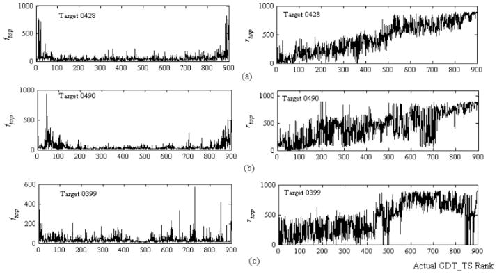
Typical distributions of rtop and ftop of 900 MUFOLD models for (a) target 0428, (b) target 0490, and (c) target 0399.
RESULTS
To verify the effectiveness of our proposed method, we applied it to two different model sets of CASP8 targets. One is the server predictions of CASP8 (available at http://www.predictioncenter.org/casp8/index.cgi) and the other is the models produced by our in-house software MUFOLD. We select the MUFOLD models from 32 targets of CASP8 as the training dataset, and the remaining 88 targets as the test dataset in both CASP8 server models and MUFOLD models.
Four metrics are selected to evaluate the performance of different methods, namely GDT_TS1, GDT_TSMean5, GDT_TS5 and Spearman Correlation. GDT_TS1 measures the GDT_TS score of the top model ranked by a QA approach; GDT_TSMean5 the average GDT_TS score of the top five ranked models; GDT_TS5 the GDT_TS of the best of the top five ranked models; and Spearman Correlation is the ranking correlation between predicted GDT_TS scores (output score of the integrated RBF model) of the models and actual GDT_TS of the models to their native structure.
Performance on MUFOLD Models
MUFOLD is our in-house software, which integrates whole and partial template information to cover both template-based and ab initio predictions in a same package [27]. We firstly test our method on MUFOLD models generated for the CASP8 targets. The comparison of our method with each individual score is listed in Table 1. Note, all the performance data in Table 1 are the average performance on 88 targets. Real Top1 means the average GDT_TS of the best models of 88 targets.
Table 1.
Comparison Results on MUFOLD Models
| Real Top1 | GDT_TS1 | GDT_TSMean5 | GDT_TS5 | Spearman Correlation | |
|---|---|---|---|---|---|
| Opus_PSP | 0.6162 | 0.5540 | 0.5576 | 0.5691 | 0.6008 |
| Opus_CA | 0.5296 | 0.5309 | 0.5534 | 0.5720 | |
| Cheng Score | 0.5444 | 0.5490 | 0.5700 | 0.5227 | |
| Dfire | 0.5509 | 0.5494 | 0.5620 | 0.5279 | |
| RAPDF | 0.5404 | 0.5418 | 0.5534 | 0.5437 | |
| RBF1 | 0.5348 | 0.5188 | 0.5577 | 0.6169 | |
| RBF2 | 0.5256 | 0.5148 | 0.5565 | 0.6106 | |
| Integrated RBF | 0.5706 | 0.5660 | 0.5790 | 0.6253 |
From the data in Table 1, we can see that among the five existing scores and two individual RBF models, the best GDT_TS1 is 0.5540 by Opus-PSP, the best GDT_TSMean5 is 0.5576 also by Opus-PSP, the best GDT_TS5 is 0.5700 by Cheng Score, and the best Spearman Correlation is 0.6169 by RBF1. Our method (integrated RBF model) outperforms any of the individual approaches by any measure significantly. The corresponding performances of our method using the four measures are 0.5706, 0.5660, 0.5790, and 0.6253, which gain 3.00%, 1.51%, 1.59% and 1.37% improvements, respectively.
More specifically, we also plot the comparison of the GDT_TS1 for 88 targets between our method and Opus-PSP (the best individual scores in both GDT_TS1 and GDT_TSMean5 metrics) in Fig. (5a). The result shows that the number of points above the diagonal, 42, is more than those below the diagonal, 27, and the other 19 points lie on the diagonal exactly. This means that overall the integrated RBF model is better than Opus-PSP. There are several cases where the improvement of integrated RBF model over Opus-PSP is substantial. Furthermore, a comparison of GDT_TS1 between the selected top model of our method and the best structure (measured by GDT_TS1) among top models ranked by each of seven individual scoring functions is shown in Fig. (5b). The figure shows that most of the points are close to the diagonal. The average of GDT_TS1 is 0.5706 and 0.5845 for selected top models of our method and the best one of the selected top models ranked by all seven individual approaches, respectively. This indicates our method can mostly recognize the best structure among top ranked models by the seven individual approaches, which might suggest our method is approaching the theoretical limit of sampling and combined discerning power of all scoring functions.
Fig. 5.
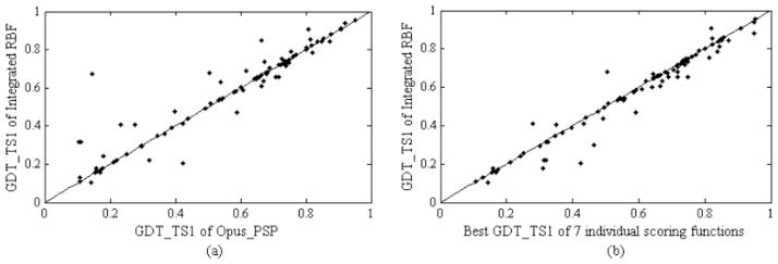
(a) Comparison of GDT_TS1 of integrated RBF and Opus-PSP; (b) comparison of GDT_TS1 of integrated RBF and the best GDT_TS1 from seven individual scoring functions on MUFOLD models.
Performance on CASP8 Server Models
We also tested our method on the CASP8 server models. Although CASP8 server prediction includes models from more than 70 diverse servers, the computational results show that our approach still works very well in this dataset. A comparison of our method versus each individual QA score is listed in Table 2. Similar to Table 1, all the performance data in Table 2 are the average performance on 88 targets and Real Top1 means the average GDT_TS of the best models of 88 targets. Table 2 shows that among the five existing scores and two individual RBF models, the best GDT_TS1 is 0.5699 by Cheng Score, the best GDT_TSMean5 is 0.5743 by Cheng Score, the best GDT_TS5 is 0.6376 by DFIRE, and the best Spearman Correlation is 0.5167 by RAPDF. In contrast, the corresponding values of the integrated RBF are 0.6093, 0.6031, 0.6489, and 0.5426, gaining 6.92%, 5.00%, 1.78% and 5.00% improvements, respectively. This result shows that the improvement of our method is significant.
Table 2.
Comparison Results on CASP8 Server Prediction
| Real Top1 | GDT_TS1 | GDT_TSMean5 | GDT_TS5 | Spearman Correlation | |
|---|---|---|---|---|---|
| Opus_PSP | 0.6845 | 0.5096 | 0.5323 | 0.6055 | 0.4951 |
| Opus_CA | 0.4720 | 0.4921 | 0.5883 | 0.4241 | |
| Cheng Score | 0.5700 | 0.5743 | 0.6289 | 0.4893 | |
| DFIRE | 0.5564 | 0.5720 | 0.6376 | 0.4507 | |
| RAPDF | 0.4792 | 0.5165 | 0.6110 | 0.5167 | |
| RBF1 | 0.5537 | 0.5739 | 0.6155 | 0.5093 | |
| RBF2 | 0.5528 | 0.5722 | 0.6004 | 0.4974 | |
| Integrated RBF | 0.6093 | 0.6031 | 0.6489 | 0.5426 |
Similarly to Fig. (5a), we plot the comparison of the GDT_TS1 for 88 targets by the best individual score in GDT_TS1/GDT_TSMean5 metrics (Cheng Score) and by our method in Fig. (6a). Similarly to Fig. (5b), we also plot the comparison of GDT_TS1 by the best structure (measured by GDT_TS1) among top models ranked by seven individual scoring functions and that by our method in Fig. (6b). Table 2 and Fig. (6) confirm that the integrated RBF model is better than each individual approach. In Fig. (6a), there are 56 and 25 points above and below the diagonal, respectively, and 7 points lie on the diagonal. The average of GDT_TS1 is 0.6093 and 0.6357 for top ranked models of our method and the best models ranked by all seven individual approaches combined, respectively. The gap is larger than that in the test using MUFOLD models (0.5706 and 0.5845, respectively). This may be due to the fact that the integrated RBF model was trained using MUFOLD models and CASP8 server models are more diverse than MUFOLD models.
Fig. 6.
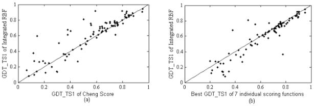
(a) Comparison of GDT_TS1 of integrated RBF and Cheng Score; (b) comparison of GDT_TS1 of integrated RBF and the best of seven individual scoring functions on CASP8 server prediction models.
DISCUSSIONS AND CONCLUSIONS
In recent CASP tests, it has been shown that meta-server methods are the most effective approaches in the field. A number of individual tools also incorporated various third-party tools to mimic meta-servers. However, in reality one typically cannot obtain so many prediction tools and get a suitable model pool. Our idea is to mimic the meta-server methods but do not need to collect or incorporate so many tools. The foundation of this approach is based on the following hypothesis: better structures are more likely to be over-represented among top ranked models in various combinations of scoring functions, given that each scoring function may evaluate some but not all aspects of structure quality well. By integrating of these scores with a large number of sampling, the resulting score is more robust and has far better chance to rank good structures on the top.
Based on the above consideration, in this paper we present a novel sampling based machine-learning method to integrate multiple existing scores and features for the protein structure QA problem. Through sampling, more robust sampling distribution features are obtained and used as the inputs of an integrated RBF model. To evaluate the ability of our novel method, we applied it to two different datasets, CASP8 server predictions and MUFOLD models. The test results show that the sampling based machine-learning method is superior to any individual QA score in all the four measurement metrics, GDT_TS1, GDT_TSMean5, GDT_TS5 and Spearman Correlation. The new method is not only useful for our own protein structure prediction development in MUFOLD, but also can be applied in any protein structure prediction tool.
Acknowledgments
The authors are grateful to the support of US National Institutes of Health (R21/R33-GM078601), the National Natural Science Foundation of China (60703025, 10872077), the science-technology development project of Jilin Province of China (20090152, 20080708), and the Special Fund for Basic Scientific Research of Central Colleges, Jilin University (421032011421). The authors like to thank Drs. Jianlin Cheng, Jianpeng Ma, John Moult, and Yaoqi Zhou for providing their scoring functions to the research community. Major computations were performed using the UMBC computing resource.
References
- 1.Baker D, Sali A. Protein structure prediction and structural genomics. Science. 2001;294:93–96. doi: 10.1126/science.1065659. [DOI] [PubMed] [Google Scholar]
- 2.Eramian D, Eswar N, Shen MY, Sali A. How well can the accuracy of comparative protein structure models be predicted? Prot Sci. 2008;17(11):1881–1893. doi: 10.1110/ps.036061.108. [DOI] [PMC free article] [PubMed] [Google Scholar]
- 3.Xu Y, Xu D. Protein threading using PROSPECT: design and evaluation. Proteins: Struct Func Bioinform. 2000;40:343–354. [PubMed] [Google Scholar]
- 4.Kim DE, Chivian D, Baker D. Protein structure prediction and analysis using the Robetta server. Nucleic Acids Res. 2004;32:526–531. doi: 10.1093/nar/gkh468. [DOI] [PMC free article] [PubMed] [Google Scholar]
- 5.Zhang Y, Skolnick J. Automated structure prediction of weakly homologous proteins on a genomic scale. Proc Nat Acad Sci USA. 2004;101:7594–7599. doi: 10.1073/pnas.0305695101. [DOI] [PMC free article] [PubMed] [Google Scholar]
- 6.Soding J, Biegert A, Lupas A. The HHpred interactive server for protein homology detection and structure prediction. Nucleic Acids Res. 2005;33:W244–W248. doi: 10.1093/nar/gki408. [DOI] [PMC free article] [PubMed] [Google Scholar]
- 7.Floudas CA. Computational Methods in Protein Structure Prediction. Biotech Bioeng. 2007;97(2):207–213. doi: 10.1002/bit.21411. [DOI] [PubMed] [Google Scholar]
- 8.Kihara D, Chen H, Yang YFD. Quality Assessment of Protein Structure Models. Curr Prot Pept Sci. 2009;10:216–228. doi: 10.2174/138920309788452173. [DOI] [PubMed] [Google Scholar]
- 9.Lazaridis T, Karplus M. Discrimination of the native from mis-folded protein models with an energy function including implicit solvation. J mol Boil. 1998;288:477–487. doi: 10.1006/jmbi.1999.2685. [DOI] [PubMed] [Google Scholar]
- 10.Still WC, Tempczyk A, Hawley RC, Hendrickson T. Semi-analytical treatment of solvation for molecular mechanics and dynamics. J Am Chem Soc. 1990;112:6127–6129. [Google Scholar]
- 11.Bowie FU, Luthy R, Eisenberg D. A method to identify protein sequences that fold into a known three-dimensional structure. Science. 1991;253:164–170. doi: 10.1126/science.1853201. [DOI] [PubMed] [Google Scholar]
- 12.Lu H, Skolnick J. A distance dependent atomic knowledge-based potential for improved protein structure selection. Proteins. 2001;44:223–232. doi: 10.1002/prot.1087. [DOI] [PubMed] [Google Scholar]
- 13.Wu Y, Lu M, Chen M, Li J, Ma J. OPUS-Ca: A knowledge based potential function requiring only Ca positions. Prot Sci. 2007;16:1449–1463. doi: 10.1110/ps.072796107. [DOI] [PMC free article] [PubMed] [Google Scholar]
- 14.Lu M, Dousis AD, Ma J. OPUS-PSP: an orientation-dependent statistical all-atom potential derived from side-chain packing. J mol Boil. 2008;376:288–301. doi: 10.1016/j.jmb.2007.11.033. [DOI] [PMC free article] [PubMed] [Google Scholar]
- 15.Zhou H, Zhou Y. Distance-scaled, finite ideal-gas reference state improves structure-derived potentials of mean force for structure selection and stability prediction. Prot Sci. 2002;11:2714–2726. doi: 10.1110/ps.0217002. [DOI] [PMC free article] [PubMed] [Google Scholar]
- 16.Samudrala R, Moult J. An all-atom distance dependent conditional probability discriminatory function for protein structure prediction. J Mol Boil. 1998;275:895–916. doi: 10.1006/jmbi.1997.1479. [DOI] [PubMed] [Google Scholar]
- 17.Cheng J, Wang Z, Tegge AN, Eickholt J. Prediction of global and local quality of CASP8 models by MULTICOM series. Proteins: Struct, Func Bioinform. 2009;77(Suppl 9):181–184. doi: 10.1002/prot.22487. [DOI] [PubMed] [Google Scholar]
- 18.Larsson P, Skwark MJ, Wallner B, Elofsson A. Assessment of global and local model quality in CASP8 using Pcons and ProQ. Proteins: Struct, Func Bioinform. 2009;77(Suppl 9):167–172. doi: 10.1002/prot.22476. [DOI] [PubMed] [Google Scholar]
- 19.Benkert P, Tosatto SCE, Schwede T. Global and local model quality estimation at CASP8 using the scoring functions QMEAN and QMEANclust. Proteins: Struct, Func Bioinform. 2009;77(Suppl 9):173–180. doi: 10.1002/prot.22532. [DOI] [PubMed] [Google Scholar]
- 20.Qiu J, Sheffler W, Baker D, Noble WS. Ranking predicted protein structures with support vector regression. Proteins. 2007;71(3):1175–1182. doi: 10.1002/prot.21809. [DOI] [PubMed] [Google Scholar]
- 21.Ginalski K, Elofsson A, Fischer D, Rychlewski L. 3D-Jury: a simple approach to improve protein structure predictions. Bioinformatics. 2003;19:1015–1018. doi: 10.1093/bioinformatics/btg124. [DOI] [PubMed] [Google Scholar]
- 22.Wang Z, Tegge AN, Cheng J. Evaluating the Absolute Quality of a Single Protein Model Using Support Vector Machines and Structural Features. Proteins. 2009;75(3):638–647. doi: 10.1002/prot.22275. [DOI] [PubMed] [Google Scholar]
- 23.Ginalski K, Rychlewski L. Protein structure prediction of CASP5 comparative modeling and fold recognition targets using consensus alignment approach and 3D assessment. Proteins. 2003;53(Suppl 6):410–417. doi: 10.1002/prot.10548. [DOI] [PubMed] [Google Scholar]
- 24.Xu D, Xu Y, Liang J. Comput Methods Prot Struct Predict Model. Vol. 2. Springer-Verlag; 2007. Protein Structure Prediction as a Systems Problem; pp. 177–206. [Google Scholar]
- 25.Yang YFD, Park C, Kihara D. Threading without optimizing weighting factors for scoring funciton. Proteins. 2008;73:581–596. doi: 10.1002/prot.22082. [DOI] [PubMed] [Google Scholar]
- 26.Zemla A. LGA: A Method for Finding 3D Similarities in Protein Structures. Nucleic Acids Res. 2003;31(13):3370–3374. doi: 10.1093/nar/gkg571. [DOI] [PMC free article] [PubMed] [Google Scholar]
- 27.Zhang JF, Wang QG, Barz B, He ZQ, Kosztin I, Shang Y, Xu D. MUFOLD: A new solution for protein 3D structure prediction. Proteins. 2009;78(5):1137–1152. doi: 10.1002/prot.22634. [DOI] [PMC free article] [PubMed] [Google Scholar]
- 28.Carroll SR, Carroll DJ. Statistics Made Simple for School Leaders. Rowman & Littlefield; Lanham: 2002. [Google Scholar]
- 29.Kabsch W, Sander C. Dictionary of protein secondary structure: pattern recognition of hydrogen-bonded and geometrical features. Biopolymers. 1983;22(12):2577–637. doi: 10.1002/bip.360221211. [DOI] [PubMed] [Google Scholar]
- 30.Jones DT. Protein secondary structure prediction based on position-specific scoring matrices. J Mol Biol. 1999;292:195–202. doi: 10.1006/jmbi.1999.3091. [DOI] [PubMed] [Google Scholar]
- 31.Dor O, Zhou Y. Real-SPINE: An integrated system of neural networks for real-value prediction of protein structural properties. Proteins. 2007;68:76–81. doi: 10.1002/prot.21408. [DOI] [PubMed] [Google Scholar]
- 32.Park J, Sandberg JW. Universal approximation using radial basis functions networks. Neural Computation. 1991;3:246–257. doi: 10.1162/neco.1991.3.2.246. [DOI] [PubMed] [Google Scholar]