7T Multi-shell Hybrid Diffusion Imaging (HYDI) for Mapping Brain Connectivity in Mice

Abstract

Diffusion weighted imaging (DWI) is widely used to study microstructural characteristics of the brain. High angular resolution diffusion imaging (HARDI) samples diffusivity at a large number of spherical angles, to better resolve neural fibers that mix or cross. Here, we implemented a framework for advanced mathematical analysis of mouse 5-shell HARDI (b=1000, 3000, 4000, 8000, 12000 s/mm²), also known as hybrid diffusion imaging (HYDI). Using q-ball imaging (QBI) at ultra-high field strength (7 Tesla), we computed diffusion and fiber orientation distribution functions (dODF, fODF) to better detect crossing fibers. We also computed a quantitative anisotropy (QA) index, and deterministic tractography, from the peak orientation of the fODFs. We found that the signal to noise ratio (SNR) of the QA was significantly higher in single and multi-shell reconstructed data at the lower b-values (b=1000, 3000, 4000 s/mm²) than at higher b-values (b=8000, 12000 s/mm²); the b=1000 s/mm² shell increased the SNR of the QA in all multi-shell reconstructions, but when used alone or in <5-shell reconstruction, it led to higher angular error for the major fibers, compared to 5-shell HYDI. Multi-shell data reconstructed major fibers with less error than single-shell data, and was most successful at reducing the angular error when the lowest shell was excluded (b=1000 s/mm²). Overall, high-resolution connectivity mapping with 7T HYDI offers great potential for understanding unresolved changes in mouse models of brain disease.

1. INTRODUCTION

Diffusion-weighted MR imaging (DWI) is a powerful tool to study water diffusion in the brain. By sampling water diffusivity at multiple spherical angles, DWI can reveal the orientational architecture of neural tissue within each voxel of the image [1, 2, 3] revealing the underlying tissue microstructure. The directions of the underlying axonal fibers can be estimated from a minimum of six independent diffusion-sensitized images, and one non-diffusion weighted image (b₀ image). These images are used in diffusion tensor imaging (DTI) to estimate a 3×3 diffusion tensor, or the covariance matrix of a 3-dimensional Gaussian distribution [3]. However, as white matter fibers mix and cross, diffusion will not always be Gaussian, and the DTI model will fail to resolve complex structures [1, 4]. In addition, with DTI it is hard to model partial volume effects (where white matter, gray matter and cerebrospinal fluid may all contribute to diffusion in the same voxel) [1, 3, 5].

To overcome some limitations of DTI, a broad spectrum of acquisition and reconstruction methods have been developed [6, 7]. High angular resolution diffusion imaging (HARDI), for example, acquires a large number of angular measures of diffusion in a “single-shell” scheme (i.e., they use a fixed diffusion weighting, or b-value). Other methods, such as diffusion spectrum imaging (DSI) [6], use a dense Cartesian sampling of a large set of possible angles and multiple b-values to resolve diffusion microstructures with a model-free approach. DSI can be time consuming as it uses a large number of measurements to encode the q-space at each voxel [4]. An alternative approach, used here, employs a multiple-shell scheme to sample diffusivity on multiple concentric spheres in q-space, each with a fixed b-value [4]. This method is referred to as multi-shell HARDI, or hybrid diffusion imaging (HYDI). Although we and others have used this method in humans [4], this paper may be the first report of HYDI in experimental mice, where longer scan times can resolve even finer structure. In these scans, voxel volumes are around 1000 times smaller than in typical human DWI scans.

In this study, we extend the power of high-field MRI to map the healthy mouse connectome. Specifically, we explored the benefits of HYDI using the q-ball imaging (QBI) model [6]. We estimated the diffusion and fiber orientation distribution functions (dODF, fODF) of the diffusion propagator [1] to investigate how each layer of complexity adds to our interpretation of tissue microstructure and fiber-based reconstructions. Understanding the complex connectivity patterns of the brain may require advanced methods, including a multi-shell scheme – especially when we try to shed light on white matter pathology. The current technology can be scaled to mouse models of disease, and importantly human imaging for improved acquisition protocols.

2. METHODOLOGY

2.1 Fiber Profile Estimation, Quantitative Anisotropy and Tractography

K-space and q-space imaging methods rely on the Fourier transform to define the relationship between the diffusion MR signal, S(k,q), average diffusion propagator, p_Δ(r,R) for time Δ, and the diffusion spin density, ρ_Δ(r) [1, 2]. From the k-space reconstruction, the diffusion weighted image can be derived, W(r,q), as a function of the average propagator at each voxel:

$$W(\mathit{r},\mathit{q})=\int \rho (\mathit{r})p_{\mathrm{\Delta }}(\mathit{r},\mathit{R})e^{(i2\pi \mathit{q}·\mathit{R})}d\mathit{R}$$ (1)

where r is the voxel coordinate, q = γGδ/2π with γ defined as the gyromagnetic ratio, and G and δ as the strength and duration of the encoding gradient; finally, R is the diffusion displacement [2]. In Eq. 1, ρ(r)p_Δ (r, R) represents the spin density function, or Q(r,R), and defines the diffusion average propagator in the scale of the spin quantity. By applying the cosine transform to Eq. 1, Q(r,R) can be redefined as:

$$Q(r,R)=\int W(r,q)cos(2\pi q·R)dq$$ (2)

From here, we can quantify the distribution of spins undergoing diffusion in a particular direction û:

$${\psi }_Q(r,\widehat{\mathrm{u}})={\int }_{}^{{\mathit{L}}_{\mathrm{\Delta }}}Q(\mathit{r},L\widehat{\mathrm{u}})\text{dL}$$ (3)

where L_Δ is the diffusion sampling length, also known as the regularization parameter [2]. Eq. 3 represents the spin distribution function (SDF) and when obtained from the spin destiny function, Q(r,R), it defines the orientation distribution function (ODF) of the spin quantity. Importantly, Eqs. 2 and 3 describe the relationship between the diffusion weighted image, W(r,q), and the SDF:

$${\psi }_Q(r,\widehat{\mathrm{u}})=L_{\mathrm{\Delta }}\int W(r,q)\mathit{sinc}(2\pi L_{\mathrm{\Delta }}q·\widehat{\mathrm{u}})\text{dq}$$ (4)

if L_Δ is set to infinity, the sinc function in Eq. 4 [2] becomes the delta function and therefore, estimates the Funk-Radon transform used by QBI [6] – also computed in this study.

The normalization of the SDF turns it into a diffusion ODF (dODF), ψ_d, which may be viewed as a linear summation of multiple dODFs and a background isotropic dODF [1]. Each dODF component may correspond to a fiber population within each voxel; they are defined here by the vertices of an 8-fold tessellated icosahedron, resulting into 642 sampling directions (dODF is symmetric around the origin, so 321 directions were considered); the dODFs were computed using the analytical QBI solution with a spherical harmonic order of 8 to ensure high angular resolution, and a recommended regularization parameter of 0.006 [8]. From the dODF peaks, the fiber orientation and profiles were computed using a single fiber component; the fODF of the fiber spin density was estimated by deconvolution [2]:

$$\rho {\psi }_d={\psi }_f\otimes {\psi }_c+{\rho }_0{\psi }_0$$ (5)

Here, ρψ_d stands for SDF (see Eqs. 3 and 4), ψ_f⊗ψ_c is the convolution between the fODF and the dODF and ρ₀ψ₀ is the background isotropic dODF. Mathematically, the deconvolution is solved by inverse matrix multiplication, Aψ_f, where A is a 321×321 matrix with column vectors describing dODFψ_c at 321 orientations [2]:

$${\psi }_f=\rho A^{-1}{\psi }_d-{\rho }_0{A}^{-1}{\psi }_0$$ (6)

We performed ODF deconvolution, with a smoothening factor of 20, as it has been shown to improve the angular resolution of the resolved fibers over the dODF [1]. Finally, we computed the quantitative anisotropy (QA) - which is a metric for each resolved fiber population (unlike FA, which is a metric for each voxel) and includes an SDF scaling factor, Z₀ [2]:

$$QA(\widehat{\mathrm{u}})=Z_0({\psi }_f(\widehat{\mathrm{u}})-I{\psi }_f)$$ (7)

Based on the spin fiber density information in the fODF, we performed deterministic streamline tractography with QA as a threshold criterion to define where fiber tracts terminate (probabilistic fiber tracking methods could also be used). As part of the implementation [1], fiber orientations were defined based on the fODF local maxima. 35,000 fibers were extracted. Reconstruction, deconvolution and tractography were performed in DSI studio (www.dsi-studio.labsolver.org) [1, 2, 5].

2.2 Data and Analysis

We analyzed a healthy (wildtype) mouse scanned ex vivo with a 7 Tesla Bruker BioSpin MRI scanner at the California Institute of Technology. DWIs were acquired using a spin echo pulse sequence (120×166×80 matrix; voxel size: 0.1×0.1×0.2 mm³, TE=34 ms; TR=500 ms, δ=11 ms, Δ=16 ms). 305 separate volumes were acquired: 5 T2-weighted volumes with no diffusion sensitization (b₀ image) and 300 diffusion-weighted images. DWIs were acquired with the same angular sampling across 5 distinct b-value shells: 1000, 3000, 4000, 8000 and 12000 s/mm² (each b-value shell contained 60 diffusion-weighted images). We designed a pre-processing protocol inspired by human processing workflows [9, 10]. First, we corrected the images for eddy current distortions using the “eddy correct FSL” tool (www.fmrib.ox.ac.uk/fsl) [12] for which a corrected gradient table was calculated to account for the distortions. Then, we removed extra cerebral tissue using the “skull-stripping” Brain Extraction Tool from BrainSuite (http://brainsuite.org/) and edited the images manually as needed. All images were linearly aligned and up-sampled to the Mori DWI template (http://cmrm.med.jhmi.edu/) (voxel size: 0.065×0.065×0.065 mm³) using FSL’s flirt function [11] with 12 degrees of freedom. Furthermore, the gradient direction table was rotated accordingly after each linear registration.

As part of our analysis, we first investigated the benefit of using multiple shells by analyzing the signal to noise ratio (SNR) of the QA computed for each individual shell, compared to multi-shell reconstructed images. The same number of samples was used within each shell to fairly compare the SNR across shells. All shells had the same angular sampling to best exploit the effects of the b-values across the shells and not the bias from the difference in angular sampling. We computed the mean SNR as the ratio between the mean voxel value within a region of interest (ROI) and the standard deviation of the voxel value within the same ROI. We delineated the ROI within the cingulum¹ of the mouse brain. For comparison purposes, we defined the 5-shell HYDI as the ‘ground truth’ and compared the performance of the reconstruction and deconvolution methods from individual shells, and <5 multi-shell HYDI (called target images), to the performance obtained from the ground truth image. To do this, we computed the largest local maximum in the fODFs within each voxel within the cingulum and determined the minimum angular deviation, or the inner angle between the fiber orientations corresponding to the local maxima, between each target image and the ground truth image:

$$\theta =\mathit{min}\left|{cos}^{-1}\right|\sum {\widehat{\mathrm{u}}}_{\mathit{max},1}·{\widehat{\mathrm{u}}}_{\mathit{max},2}\Vert$$ (8)

Here, û_{max, 1} and û_{max, 2} are the local maxima peaks within a voxel in the ground truth and target images.

3. RESULTS

As expected, the mean SNR of the single-shell QA (Fig. 1) in the mouse cingulum was highest at the lowest b-value and decreased, for single-shell acquisitions, as the b-value increased (Fig. 2). In a 2-tailed t-test, we found that the mean SNR within the cingulum in the single- and 2-shell DWIs is significantly higher at the b-value range 1000–4000 s/mm², compared to the b-value range 8000–12000 s/mm² (p-value=0.02). This has been previously shown in human data [13], and is expected here as the noise increased with increasing b-values, possibly affecting the shape of the fODFs used for the QA computation. Meanwhile, as we reconstructed the 2+ multi-shell HYDIs, adding the lowest b-value shell (b-value= 1000 s/mm²) significantly increased the SNR (p-value=0.02); note the visibly nosier QA and fiber reconstruction at b-value=1000 s/mm² in Figures 1 and 3. On the other hand, we found that the highest b-value shell (b-value=12000 s/mm²) did not significantly impact the SNR of the multi-shell QA although the fiber reconstruction seems visibly more similar to the ground truth image reconstruction (Fig. 3).

Figure 1.

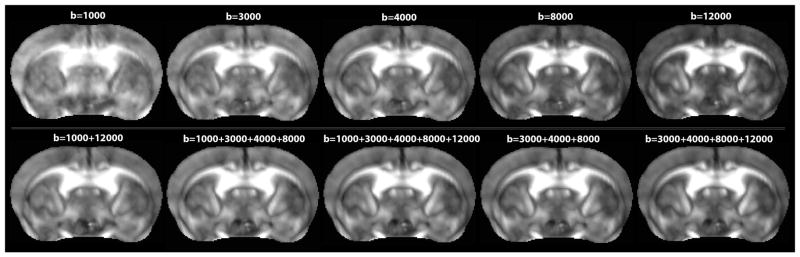
Quantitative fractional anisotropy (QA) maps computed for single- and multi-shell DWI acquisitions in the mouse brain. The contrast to noise ratio visibly increases with the b-value shell, while the highest signal to noise ratio (SNR) is found in the lowest b-values shells (especially at b-value=1000 s/mm²).

Figure 2.

The signal to noise ratio (SNR) of quantitative anisotropy (QA) in single and multi-shell DWIs in the mouse cingulum is plotted. The same set of angular samples was used for each single- and multi-shell reconstruction. The lowest diffusion weighting gives the highest SNR.

Figure 3.

Deterministic streamline fiber tracts computed from QBI, as a function of fiber spin density, based on single and multi-shell DWIs in a coronal slice of the mouse brain. Tracts are overlaid on the fiber ODF maps; 5-shell HYDI was selected as ‘ground truth’ for comparison purposes. Note the poor resolution of fiber directions at b=1000 s/mm², the value typically used in human studies today.

Although the lowest b-value shell (b=1000 s/mm²) adds more signal to the QA, it also adds more angular error to the resolved fiber population in the cingulum (Figs. 3 and 4). In contrast to the 5-shell HYDI ground truth image, the angular deviation of the major peak fibers in the b=1000 s/mm² shell across 64 voxels was as high as 53° (Fig. 4). A 53° angular error can occur when the anterior-to-posterior fibers of the cingulum are confused as being part of the corpus callosum (left-to-right directionality), which is what we observe in Figures 3 and 4 (fibers in the cingulum are slightly red). Mean angular errors across all single-shell data were significantly higher than the errors from multi-shell HYDI, but only when the b=1000 s/mm² shell was excluded from the multi-shell reconstruction (2-tailed t-test p-value=0.02). Lowest angular errors were achieved for major fibers reconstructed from the last three shells (b=4000, 8000, 12000 s/mm²), however, reconstruction from the middle shells performed comparably well (b=3000, 4000, 8000 s/mm² and b=4000, 8000 s/mm²).

Figure 4.

Top row fODFs and zoomed in tracts at b=1000 s/mm², and separately, in a 5-shell ‘ground truth’ HYDI, illustrated in the cingulum of the mouse brain across 64 voxel (8×8). 2^nd and 3^rd rows: 8×8 matrix showing angular error (0°–53°) between local maxima of fiber peaks (fODFs) in the cingulum at voxel level for target images and the ‘ground truth’ image. Angular error is highest at b=1000 s/mm² and decreases as shells are combined (p=0.02). The agreement with ground truth increases from the left to the right in the 2^nd and 3^rd rows. Angular deviation as high as 53° can occur when the anterior-to-posterior fibers of the cingulum are confused as being part of the corpus callosum that have a left-to-right directionality.

4. CONCLUSION

In this work, we explore the benefits of high-field multi-shell diffusion imaging, or HYDI, to understand how each distinct b-value shells adds to the complexity of the reconstructed diffusion signal. We show that 7T HYDI is feasible in mice, and the effects of different q-space sampling methods at single-shell b-values 1000, 3000, 4000, 8000 and 12000 s/mm², as well as a combination of multi-shell schemes.

We found that excluding the b-value=1000 s/mm² shell improves the fiber reconstruction accuracy and importantly, also saves scanning time. This particular b-value shell is the most frequently used in human imaging studies today – so studying its added value is important. For improved fiber peak orientation accuracy, adding higher b-value shells proved to be beneficial (i.e., b-value=3000, 4000, 8000 s/mm²). For instance, multi-shell HYDI reconstructions composed of b-value shells 4000 s/mm² and 8000 s/mm² were almost as accurate as the 5-shell HYDI ground truth reconstruction. This further indicates that not all 5-shells are necessary to acquire a highly complex and accurate diffusion signal, which once again – allows us to save scanning time.

To reconstruct the diffusion signal, we used fODFs – the orientation distribution of the fiber spins [1, 2, 5], which better resolve crossing fibers and fiber peaks. In fact, fODFs obtained from spherical deconvolution, as computed here, have been claimed to be more accurate than dODFs and other methods [1, 8]. This deconvolution method can be applied to ODFs obtained from many other reconstruction methods including DSI [6], generalized q-sampling imaging (GQI) [2], and others. Other reconstruction methods may lead to different fiber reconstruction outcomes, so results should still be interpreted cautiously.

HYDI offers an unprecedented power to assess the structural connectivity and neural integrity of the mouse brain – especially for studies that aim to validate the diffusion signal with high-resolution histological correlates. Despite the popularity of DWI, a lack of histological ground truth makes it difficult to understand the cellular basis of the underlying neuroimaging signals. Our future work will integrate the highly complex diffusion signal from HYDI with ex vivo cellular measures, and will assess the potential of connectivity analysis for assessing therapeutic consequences.

References

- 1.Yeh FC, Wedeen VJ, Tseng WY. Estimation of fiber orientation and spin density distribution by diffusion deconvolution. Neuroimage. 2011;55(3):1054–62. doi: 10.1016/j.neuroimage.2010.11.087. [DOI] [PubMed] [Google Scholar]
- 2.Yeh FC, Wedeen VJ, Tseng WY. Generalized q-sampling imaging. IEEE Trans Med Imaging. 2010;29(9):1626–35. doi: 10.1109/TMI.2010.2045126. [DOI] [PubMed] [Google Scholar]
- 3.Basser PJ, Pierpaoli C. Microstructural and physiological features of tissues elucidated by quantitative-diffusion-tensor MRI. J Magn Reson. 1996;213(2):560–70. doi: 10.1016/j.jmr.2011.09.022. [DOI] [PubMed] [Google Scholar]
- 4.Zhan L, Leow AD, Aganj I, Lenglet C, Sapiro G, Yacoub E, Harel N, Toga AW, Thompson PM. Differential information content in staggered multiple shell HARDI measured by the tensor distribution function. IEEE ISBI. 2011:305–309. [Google Scholar]
- 5.Yeh FC, Tseng WYI. Sparse solution of fiber orientation distribution function by diffusion decomposition. Plos One. 2013;8(10):e75747. doi: 10.1371/journal.pone.0075747. [DOI] [PMC free article] [PubMed] [Google Scholar]
- 6.Tuch DS. Q-ball Imaging. Magn Reson Med. 2004;52:1358–1372. doi: 10.1002/mrm.20279. [DOI] [PubMed] [Google Scholar]
- 7.Wedeen VJ, Hagmann P, Tseng WY, Reese TG, Weisskoff RM. Mapping complex tissue architecture with diffusion spectrum magnetic resonance imaging. Magn Reson Med. 2005;54(6):1377–86. doi: 10.1002/mrm.20642. [DOI] [PubMed] [Google Scholar]
- 8.Descoteaux M, Angelino E, Fitzgibbons S, Deriche R. Regularized, fast, and robust analytical Q-ball imaging. Magn Reson Med. 2007;58(3):497–510. doi: 10.1002/mrm.21277. [DOI] [PubMed] [Google Scholar]
- 9.Daianu M, Jahanshad N, Nir TM, Toga AW, Jack CR, Weiner MW, Thompson PM the Alzheimer’s Disease Neuroimaging Initiative. Breakdown of Brain Connectivity between Normal Aging and Alzheimer’s Disease: A Structural k-core Network Analysis. Brain Connectivity. 2013;3(4):407–22. doi: 10.1089/brain.2012.0137. [DOI] [PMC free article] [PubMed] [Google Scholar]
- 10.Daianu M, Jahanshad N, Nir TM, Leonardo CD, Jack CR, Weiner MW, Bernstein M, Thompson PM. Algebraic connectivity of brain networks shows patterns of segregation leading to reduced network robustness in Alzheimer’s disease. MICCAI Computational Diffusion MRI (CDMRI) Workshop; Boston, MA, USA. 2015. In Press. [DOI] [PMC free article] [PubMed] [Google Scholar]
- 11.Jenkinson M, Bannister P, Brady M, Smith S. Improved optimization for the robust and accurate linear registration and motion correction of brain images. Neuroimage. 2002;17:825–841. doi: 10.1016/s1053-8119(02)91132-8. [DOI] [PubMed] [Google Scholar]
- 12.Smith SM. Fast robust automated brain extraction. Hum Brain Mapp. 2002;17:143–155. doi: 10.1002/hbm.10062. [DOI] [PMC free article] [PubMed] [Google Scholar]
- 13.Khachaturian MH, Wisco JJ, Tuch DS. Boosting the sampling efficiency of q-ball imaging using multiple wavevector fusion. Magn Reson Med. 2007;57(6):289–296. doi: 10.1002/mrm.21090. [DOI] [PubMed] [Google Scholar]