A Primer to Single-Particle Cryo-Electron Microscopy

Summary

Cryo-electron microscopy (cryo-EM) of single-particle specimens is used to determine the structure of proteins and macromolecular complexes without the need for crystals. Recent advances in detector technology and software algorithms now allow images of unprecedented quality to be recorded and structures to be determined at near-atomic resolution. However, compared with X-ray crystallography, cryo-EM is a young technique with distinct challenges. This primer explains the different steps and considerations involved in structure determination by single-particle cryo-EM to provide an overview for scientists wishing to understand more about this technique and the interpretation of data obtained with it, as well as a starting guide for new practitioners.

Introduction

Cryo-electron microscopy (cryo-EM) has the ability to provide 3D structural information of biological molecules and assemblies by imaging non-crystalline specimens (single particles). Although the development of the cryo-EM technique began in the 1970s, in the last decade the achievement of near-atomic resolution (<4Å) has attracted wide attention to the approach.

The remarkable progress in single-particle cryo-EM in the last two years has primarily been enabled by the development of direct electron detector device (DDD) cameras (Faruqi and McMullan, 2011; Li et al., 2013a; Milazzo et al., 2011). DDD cameras have a superior detective quantum efficiency (DQE), a measure of the combined effects of the signal and noise performance of an imaging system (McMullan et al., 2009), and the underlying complementary metal-oxide semiconductor (CMOS) technology makes it possible to collect dose-fractionated image stacks, referred to as movies, that allow computational correction of specimen movements (Bai et al., 2013; Campbell et al., 2012; Li et al., 2013a). Together, these features produce images of unprecedented quality, which, in turn, improves the results of digital image processing. In parallel, the continually increasing computer power allows the use of increasingly sophisticated image processing algorithms, resulting in greatly improved and more reliable 3D density maps (see also Cheng, 2015, this issue).

Much effort has been invested in simplifying and automating the collection of EM images and the use of image processing software (reviewed in Lyumkis et al., 2010). The problematic issue with single-particle EM, however, is that there is still no objective quality criterion that is simple and easy to use, such as the R-free value in X-ray crystallography, that would allow one to assess whether the determined density map is accurate or not. Even the resolution of a density map remains subject to controversies. The remaining unresolved issues may not always be fully appreciated by new practitioners and, if overlooked, can lead to questionable results. A recent example is the 6Å resolution structure of the HIV-1 envelope glycoprotein (Mao et al., 2013), which prompted a number of commentaries questioning the validity of the structure (Henderson, 2013; Subramaniam, 2013; van Heel, 2013). This primer seeks to inform about the practical nuts and bolts behind determining a structure by single-particle cryo-EM and to guide new practitioners through the workflow (Figure 1) and important caveats and considerations. Also, as these authors’ opinions may not always be shared by everybody in the field, the reader is encouraged to consult other texts on single-particle EM, such as Bai et al., 2015; Frank et al., 2006; Lau and Rubinstein, 2013, Milne et al., 2013; and Orlova and Saibil, 2011.

Figure 1. The Steps Involved in Structure Determination by Single-Particle Cryo-EM.

A single-particle project should start with a characterization of the specimen in negative stain (left arm of the workflow). Only once the EM images, or potentially 2D class averages, are satisfactory, i.e., the particles are mono-disperse and show little aggregation and a manageable degree of heterogeneity (“low-resolution” sample refinement), is the sample ready for analysis by cryo-EM (right arm of the workflow). The images, 2D class averages and 3D maps obtained with vitrified specimens may indicate that the sample requires further improvement to reach near-atomic resolution (“high-resolution” sample refinement).

Protein purification for single-particle cryo-EM

Single-particle EM depends on the computational averaging of thousands of images of identical particles. If particles exhibit variable conformation or composition (heterogeneity) more homogeneous subsets can be generated using classification procedures (more below). However, whenever possible, structural heterogeneity should be minimized through biochemical means to simplify structure determination. Biochemical analyses by SDS-PAGE and gel-filtration chromatography are not sufficient to assess whether a sample is suitable for EM analysis, as apparently intact complexes can be a mixture of compositionally different sub-complexes, and even compositionally homogeneous complexes can potentially adopt many different conformations. The most informative way to judge the quality of a protein sample is to visualize it by negative-stain EM. In addition to providing high contrast, the negative staining procedure also tends to induce proteins to adsorb to the carbon film in one or only few preferred orientations, making it easier to assess sample homogeneity (Ohi et al., 2004). The kind of information negative-stain EM provides is described in Supplemental Information.

Structural heterogeneity can be caused by compositional or conformational variability of the target. Compositional heterogeneity, typically the result of sub-stoichiometric components or dissociation of loosely associated subunits, can be addressed in various ways. Ideally, buffer conditions can be found that stabilize the target complex. A promising approach to identify suitable buffer conditions is the Thermofluor-based screening approach (Ericsson et al., 2006). In the case of a sub-stoichiometric subunit, this subunit can be tagged for affinity purification, thus increasing the fraction of complexes containing it in the final preparation. An approach that has proven useful in reducing compositional heterogeneity is mild chemical cross-linking with glutaraldehyde. More control over the cross-linking reaction is obtained with the GraFix technique, in which the sample is centrifuged into a combined glycerol/glutaraldehyde gradient (Kastner et al., 2008). A variation of this approach is “on column” cross-linking, in which the sample is cross-linked over a size-exclusion column (Shukla et al., 2014). Whichever approach is used, one must keep in mind that cross-linking can introduce artifacts. For example, flexible extensions can become glued together, resulting in a non-physiological structure. Also, if a complex can adopt different conformations, cross-linking can stabilize just one particular state, typically the most compact organization (e.g., Shukla et al., 2014). Hence, native sample always has to be analyzed, too, to understand how cross-linking affects the structure of the target.

Conformational heterogeneity tends to be more difficult to overcome, especially if one or several domains are flexibly tethered to the remainder of a protein. In this case, structural analysis may be restricted to negative-stain EM studies. Alternatively, chemical cross-linking can potentially be used to minimize the conformational heterogeneity, but the physiological relevance of the resulting structures will have to be carefully assessed. Another way to reduce conformational heterogeneity is to lock the target in a defined functional state, which can sometimes be accomplished by adding substrates, inhibitors, ligands, co-factors or any other molecule affecting the function of the target.

The greatly improved image quality provided by DDD cameras and the availability of ever more sophisticated image-processing software have made structural heterogeneity more manageable. Still, investing time to minimize structural heterogeneity by biochemical tools will always simplify subsequent image processing steps, and it will substantially reduce the risk of obtaining incorrect density maps. Every new project should thus always start with an optimization phase, in which negative-stain EM is used as a tool to optimize protein purification (Figure 1). In rare cases, negative staining will introduce artificial heterogeneity. The only option to exclude this possibility is to look at vitrified specimens by cryo-EM.

Specimen preparation for single-particle cryo-EM

Before a biological specimen can be imaged, it has to be prepared so it survives the vacuum of the electron microscope, which causes sample dehydration, and the exposure to electrons, which results in radiation damage (the deposition of energy on the specimen by inelastic scattering events that causes breakage of chemical bonds and ultimately structural collapse). The most commonly used preparation techniques, negative staining and vitrification, are briefly discussed in Supplemental Information.

Specimens used for single-particle EM usually consist of purified sample on a carbon film with a support structure. The support structure is most commonly a copper grid, and the carbon film can either be a continuous film, typically used to prepare negatively stained samples, or a holey film, commonly used to prepare vitrified specimens. A problem with EM grids is that thin carbon films are not very stable and are poor conductors at low temperature. This is thought to contribute to the occurrence of beam-induced movement, which can degrade image quality. Therefore, different grid designs have been explored to increase the conductivity of EM grids, such as using doped silicon carbide as the substrate (Cryomesh; Yoshioka et al., 2010), and to make them more mechanically stable, such as using gold support (Russo and Passmore, 2014). Before the specimen can be applied, grids have to be rendered hydrophilic, which is typically done with a glow discharger (or, less commonly, with a plasma cleaner).

A perfect vitrified specimen is characterized by an amorphous ice layer of sufficient thickness to accommodate the particles (but ideally not much thicker so that particles are clearly visible), and particles that are well distributed across the field of view and adopt a wide range of orientations. A thin layer of vitrified ice is reasonably transparent and allows particles to be seen clearly (Figures 2 and S1A), while crystalline ice adds a strong texture of dark contrast (bend contours) that usually disguises the embedded particles (Figure S1B).

Figure 2. Single-Particle Cryo-EM Images with Motion Correction.

Most data recorded with DDD cameras are dose-fractionated image stacks (movies) that can be motion-corrected.

(A) A typical cryo-EM image of vitrified archaeal 20S proteasome particles embedded in a thin layer of vitreous ice. The image is the sum of the raw movie frames without motion correction.

(B) Trace of motion of all movie frames determined using a whole-frame motion-correction algorithm (Li et al., 2013a). Note that the movement between frames is large at the beginning but then slows down.

(C) The left panel shows the power spectrum calculated from the sum of the raw movie frames without motion correction. The right panel shows the power spectrum calculated from the sum of movie frames after motion correction. Motion correction restores Thon rings to close to 3Å resolution (dashed circle).

(D) Sum of the movie frames that were shifted according to the shifts shown in (B). Note that the images shown in (A) and (D) are indistinguishable by eye, but differ significantly in the quality of the Thon rings seen in their power spectra (C).

Semi-automated plungers, such as Vitrobot (FEI) and Cryoplunge (Gatan), have made it much easier to reproducibly obtain high-quality vitrified specimens. However, care has to be taken to transfer the grids quickly between plunger and cryo-specimen holder and to minimize exposing the liquid nitrogen to air to avoid ice contamination (Figure S1C). An occasional problem is ice that has the appearance of “leopard skin” (Figure S1D). It is unclear what causes this pattern and how it can be avoided, but particles picked from images of such ice areas can still yield reliable 3D maps.

The ice layer should be as thin as possible to achieve high contrast between the molecule and the surrounding ice layer and to minimize defocus spread due to different heights of the molecules in the ice layer, which can hamper high-resolution structure determination. Importantly, if particles cannot be seen reasonably easily by eye, the sample should not be used for data collection. Parameters that affect ice thickness are described in Supplemental Information. The ice layer usually tends to be thicker around the edge of a hole and thinner in the center. Large molecules, such as viruses and ribosomes, may thus be excluded from the center of a hole. This effect is stronger with specimens containing detergent, which lowers the surface tension, making it more challenging to produce thin ice. In this case, it helps to use holey carbon grids with smaller holes.

A good vitrified specimen shows a high density of molecules in different orientations. Many particles in a hole reduces the number of images that have to be collected, but ideally the molecules should not touch each other. A problem that is often encountered is that only very few molecules are observed in the holes of the carbon film. A large percentage of molecules is removed during blotting with filter paper, and preparation of vitrified specimens thus requires a much higher sample concentration than preparation of negatively stained specimens. It is not unusual, however, that even with very highly concentrated samples, few particles are seen in the holes. Reasons for this problem can be that the molecules preferentially adsorb to the carbon film, diluting them from the holes, or that they denature as they come into contact with the air/water interface due to the surface tension. An effective solution to deal with the preferential adsorption to the carbon film is to apply the sample twice. The first application will saturate the carbon film with protein, and it is therefore more likely that more particles remain in the holes when the sample is applied a second time. Alternatively, the grid can be covered by a thin carbon or graphene support film or by a lipid monolayer to which the molecules can adsorb. However, with the exception of graphene, additional support films will reduce image contrast, and all substrates have the potential to induce molecules to adopt preferred orientations. Finally, the grid can be decorated with a self-assembled monolayer to pacify the support film and drive the molecules into the holes (Meyerson et al., 2014). Protein denaturation at the air/water interface can be addressed by using thicker ice (which will, however, reduce image contrast), by using a support film that adsorbs the molecules (but also reduces image contrast), or by chemically fixing the sample before vitrification (which has the potential, however, to affect the structure).

Occasionally particles adopt preferred orientations, presumably due to interactions with the air/water interface. This causes a problem for the reconstruction of a 3D density map, which requires multiple views. One can attempt to overcome this problem by using thicker ice, by adding low amounts of detergent (lowering the surface tension of the air/water interface), or by using a thin support film to which the molecules can adsorb and which will thus keep them away from the air/water interface. One can also try to change the glow-discharge parameters or to modify the protein, e.g., by adding/removing affinity tags. If none of these approaches are successful, it is possible (but technically very challenging) to collect images of tilted specimens, but this usually prevents achieving high resolution.

Image acquisition for single-particle cryo-EM

Structure determination by single-particle cryo-EM, especially if near-atomic resolution is targeted, requires acquisition of high-quality images, i.e., images with high contrast and with sufficient resolution to answer the biological questions being asked. In addition, particularly for high-resolution projects, high efficiency is beneficial to make them economical, i.e., one should be able to collect a large number of micrographs within a reasonable timeframe. Thus, automation of key steps may be called for. While modern electron microscopes are capable of delivering resolutions better than 2Å, collection of good-contrast, high-resolution images of vitrified specimens remains challenging. It is therefore critical not only to align the electron microscope with great care but also to choose appropriate imaging conditions. Adjustable settings include, but are not limited to, selection of the condenser aperture and spot size, reduction of imaging aberration by coma-free alignment (all briefly discussed in Supplemental Information), as well as issues related to the optimization of image contrast, such as appropriate defocus settings, selection of objective aperture, and the electron dose used. To learn about contrast enhancement by using phase plates, the reader is referred to Glaeser (2013).

The contrast of vitrified biological specimens is very low, and if images were taken in focus, they would contain little, if any, useful information. Images are therefore taken in bright-field mode of the electron microscope while applying underfocus (Frank, 2006). Given a thin object, images are linear projections of the Coulomb potential of the specimen, the fundamental property necessary for subsequent computational reconstruction of its 3D structure. The images are modulated by the Contrast Transfer Function (CTF), a quasi-periodic sine function in reciprocal space, the periodicity of which depends, among other parameters, on the defocus setting (Wade, 1992; and Supplemental Information). Furthermore, the amplitudes of the high spatial frequencies (high-resolution detail) in an image are attenuated by an envelope function of the CTF. Its rate of decline depends on the spatial coherence of the electron beam, and it increases with increasing image defocus. Therefore, a higher defocus boosts the low-resolution image contrast but weakens the high-resolution contrast, limiting the frequency range of useful information. Thus, it is best to use the smallest possible defocus that still creates sufficient low-resolution image contrast to clearly see the particles. This means that for large molecules, e.g., viruses, a small underfocus can be used. For small particles (molecular mass less than 200 kDa), however, it is often necessary to underfocus by a few micrometers, which will limit the resolution that can be achieved. Importantly, as the CTF has multiple zero crossings, some information within a single image is lost, which is the reason why images have to be collected at different underfocus settings to sample the entire reciprocal space (Penczek, 2010a; Zhu et al., 1997).

The use of an objective aperture increases amplitude contrast by cutting off electrons scattered at high angles. However, as it also sets a cut-off limit for the resolution, a relatively large objective aperture has to be used for high-resolution single-particle cryo-EM imaging (e.g., 70 μm or 100 μm).

Using a higher electron dose also increases image contrast, but higher electron doses will increase radiation damage. Therefore, for single-exposure images and to achieve high resolution, the electron dose is typically kept below ~20 e⁻/Ų. Much higher electron doses can be used when movies are recorded (see below). The dose rate also needs to be considered and depends on the type of detector being used for imaging. For imaging on film or when a charge-coupled device (CCD) camera is used, a high dose rate (high beam intensity) is typically used to keep the exposure short (~1 sec or less), which minimizes the extent of specimen drift during exposure. Short exposures are also preferred when integrating DDD cameras are used to collect single-exposure images, but longer exposures can be used when they are operated in movie mode, which reduces or eliminates the problem of specimen drift (see below). The situation is different for electron-counting DDD cameras. To ensure that electrons are counted properly, the dose rate must be kept below ~10 e⁻/pixel/sec (based on current technology) on the camera (Li et al., 2013b; Ruskin et al., 2013). Higher dose rates adversely affect electron counting, thus lowering the DQE and image contrast.

A factor contributing to the recent improvement of attainable resolution in cryo-EM is the movie mode available on some DDD cameras. Here, the total electron dose is fractionated into a series of image frames that can be aligned to compensate for specimen drift and beam-induced movement, thus reducing image blurring (Figure 2) (Brilot et al., 2012; Campbell et al., 2012; Li et al., 2013a). After alignment, the frames are averaged, and the resulting image is used for subsequent structure determination. Movies are made possible by the fast readout and the “rolling shutter” mode of CMOS detectors that underlie all DDD cameras and some newer scintillator-based cameras. Some software packages also allow for sub-frame alignment to account for local motions that occur during beam exposure (Rubinstein and Brubaker, 2014; Scheres, 2014). Movies also offer the possibility to optimize the overall Signal-to-Noise Ratio (SNR) in images of specimens affected by radiation damage. Early frames correspond to a low electron dose and therefore contain high-resolution signal from the least damaged specimen. However, early frames are also often still affected by fast specimen movement (Figure 2B), blurring the high-resolution information. While specimen movement typically slows down and affects later frames less, these correspond to a higher accumulated dose and increasingly lack high-resolution information. When movie frames are averaged, a relative weighting can be applied that optimizes the signal in the final average (Campbell et al., 2012; Scheres, 2014). As an intermediate measure to improve high-resolution image contrast, one can exclude the initial two or three frames (which are often still affected by high initial specimen movement), as well as the later frames that correspond to a total dose of ~20 e⁻/Ų and higher from the frame averages. However, this strategy results in the loss of low-resolution contrast. Therefore, it may currently be best to use images containing all the movie frames in the alignment step during image processing and to use images without the initial and final frames to calculate the final 3D map (Li et al., 2013a).

The attainable resolution depends on the pixel size on the specimen level, which, in turn, depends on the effective magnification. The physical pixel sizes of digital cameras vary as well as the exact position of the cameras in the optical path. Therefore, the image pixel size has to be calibrated not only for each magnification but also for every microscope/camera combination (a protocol for how to calibrate the magnification is described in Supplemental Information). The Nyquist theorem specifies that the theoretically attainable resolution is limited to twice the pixel size, but interpolation errors induced by image processing operations and low DQE values of the detector near the Nyquist frequency limit the practically attainable resolution further (Penczek, 2010b). As a rule of thumb, the practical resolution limit is closer to three times the pixel size.

Image processing

A significant part of the workload of a single-particle project is taken up by the processing of the recorded images. The main steps are discussed here, including correction of the microscope CTF, selection of particles and preparation of image stacks, generation of an initial structure and its refinement, treatment of structural heterogeneity, assessment of resolution, and interpretation of the final 3D density maps. A number of software packages exist that have been developed over the last four decades and are still being improved. While the development of software is important for the success of single-particle cryo-EM, the recent groundbreaking results are primarily due to the use of direct detectors and the recording of movies. Prior to their common use, none of the currently employed algorithms and software packages was capable of yielding results comparable to what is now possible. After direct detectors and movies were adopted, near-atomic resolution was achieved with several software packages, including SPIDER (Frank et al., 1981), EMAN2 (Tang et al., 2007), FREALIGN (Grigorieff, 2007), RELION (Scheres, 2012), and SPARX (Hohn et al., 2007). To date, EMAN/EMAN2 has been, and continues to be, the most popular software, owing to its extensive options, flexibility, and user friendliness. However, users new to cryo-EM may find it easier to start with more specialized software, such as RELION, which offers streamlined processing with fewer options and one main algorithmic approach (maximum likelihood). This primer is not meant to serve as a manual for any specific image processing software package, but instead tries to relate basic concepts, which may be implemented in different ways in different software packages.

Estimation of CTF parameters and correction for its effects

The accurate estimation of CTF parameters is important for both the initial evaluation of micrograph quality and subsequent structure determination. To calculate the CTF, the parameters that have to be known are acceleration voltage, spherical aberration, defocus, astigmatism and percentage of amplitude contrast. Voltage and spherical aberration are instrument parameters that are usually used without further refinement (although the value for the spherical aberration provided by the manufacturer may not be completely accurate). The defocus is set during data collection, but the setting is only approximate. More accurate values for defocus and astigmatism are obtained by fitting a calculated CTF pattern (e.g., Mindell and Grigorieff, 2003) to the Thon rings (semi-circular intensity oscillations induced by the CTF seen in the power spectrum of the image (Thon, 1966)). The contribution of the amplitude contrast is typically assumed as 5–10% for cryo-EM images.

Once the CTF parameters have been determined and as long as a set of particle views that differ by defocus settings is available, correction for the CTF effects is possible and straightforward (Penczek, 2010a). It can be done for both amplitudes and phases (full CTF correction) or only for the phases (phase flipping). For more detail on CTF estimation and correction, see Supplemental Information.

Ultimately, the determined 3D structure should be corrected for the reciprocal space envelope functions that suppress high-frequency information, and thus visual resolvability of map details. These envelope functions describe effects of microscope optics, limitations of digital scanners and cameras, and errors in orientation parameters assigned to particle images (Jensen, 2001, and section on power spectrum adjustment in Supplemental Information).

Particle picking

Once a dataset has been collected, movies have been aligned and averaged (if applicable) and good micrographs have been selected (e.g., based on Thon rings being visible to high resolution in all directions), a project continues with the labor-intensive process of particle picking. The quality of the selected particles is a major factor in the subsequent analysis, as inclusion of too many poor particles may preclude successful structure determination. Moreover, methods aimed at cleaning up the selected particles are not very robust, and many artifacts pass all tests and adversely affect subsequent data processing efforts. Particles can be selected in a manual, semi-automated, and fully automated manner. In the early stages of analysis, particularly when little is known about the shape of the protein and the distribution of the projection views, the manual approach is preferable. A trained and careful practitioner can obtain much better results than automated approaches, but the risk is that humans tend to focus on more familiar and better visible particle views, thus omitting less frequently appearing orientations that may be needed for successful structure determination. In semi-automated approaches, the computer performs an initial step of detection of putative particles in a micrograph. All candidates are windowed, and the user removes poor particles from the gallery of possible candidates. Fully automated procedures can be divided into three groups: those that rely on ad hoc steps of denoising and contrast enhancement followed by a search for regions of a given size that emerge above the background level (Adiga et al., 2004), those that extract orientation-independent statistical features from regions of micrographs that may contain particles and proceed with classification (Hall and Patwardhan, 2004; Lata et al., 1995), and those that employ templates, i.e., either class averages of particles selected from micrographs or projections from a known 3D structure of the complex (Chen and Grigorieff, 2007; Huang and Penczek, 2004; Sigworth, 2004). The use of fully automated procedures carries even higher risks of introducing bias, as positively correlating noise features are indistinguishable from weak but valid signal. Therefore, one faces the risk of eventually merely reproducing the template structure. The study of the HIV-1 envelope glycoprotein is a prominent example in which template bias likely played a deciding role (Mao et al., 2013). Good practice is therefore to rely on template-based particle picking only if particles are clearly visible in the micrographs.

With particle coordinates identified in the micrographs, the particles are windowed and assembled into a stack. The initial locations are not very precise. Therefore, the window size should exceed the approximate particle size by at least 30% (more for small particles). For issues relating to aliasing and density normalization, see Supplemental Information.

2D clustering and formation of class averages

The first step in single-particle EM structure determination is the analysis of the 2D image dataset, particularly the alignment and grouping of the data into homogenous subsets. There are several reasons for why it is best to begin with 2D analysis: (1) 2D datasets contain image artifacts, invalid particles, or simply empty fields that should be removed, (2) the angular distribution of the particle views is unknown and if the set is dominated by just a few views, 3D analysis is unlikely to succeed, and (3) computational ab initio 3D structure determination requires high-SNR input data, as is present in high-quality class averages.

Various strategies have been proposed to deal with the problem of alignment and clustering of large sets of single-particle EM images (Joyeux and Penczek, 2002; Penczek, 2008), but all are fundamentally rooted in the popular K-means clustering algorithm (Figure 3A). As most steps in single-particle EM analysis use a variant of this algorithm, including 2D multi-reference alignment, 3D multi-reference refinement, even 3D structure refinement (projection matching), the principles and properties of K-means clustering are described in Supplemental Information.

Figure 3. Principle of the K-means Algorithm Used in Single-Particle EM Structure Determination Protocols.

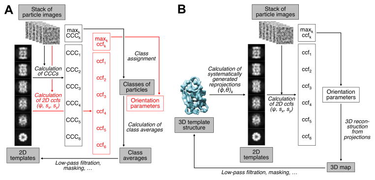
(A) In the basic K-means algorithm, the particle images are compared with a set of class averages using a correlation measure that yields the class assignment. Based on the updated class assignments, new class averages are then calculated. Simply by adding 2D alignment of the images to the templates using a correlation function, the algorithm is converted to Multi-Reference Alignment (MRA) (indicated by text in red font).

(B) Principle of the projection matching technique used for 3D single-particle EM structure refinement. The best match of an image to a template yields the Euler angles that were used to generate the template, while a 2D alignment step yields the third, in-plane Euler angle and the two in-plane translations, the total of five orientation parameters required for 3D reconstruction step.

A straightforward implementation of the K-means algorithm in single-particle EM analysis is 2D Multi-Reference Alignment (MRA) (van Heel and Stoffler-Meilicke, 1985), a process in which the dataset is presented with K seed templates, and all images are aligned to and compared with all templates and assigned to the one they most resemble. The process is iterative: a new set of templates is computed by averaging images based on results from the initial grouping (including transformations given by alignment of the data in the previous step), and the whole procedure is repeated until a stable solution is reached. To accelerate the procedure, one can employ an additional step of Principal Component Analysis (PCA) executed so that the clustering is actually performed using factorial coordinates, not the original images (for in-depth reading, see Frank, 2006). All major single-particle EM software packages contain a version of MRA, often with various heuristics aimed at improved performance, particularly with respect to the problem of “group collapse”: as MRA combines alignment with clustering, the process is unstable in that the more common particle views produce large, high-SNR class averages, which in turn “attract” less common or more noisy images, eventually leading to the disappearance of less populous groups.

In light of the fundamental shortcomings of MRA (see Supplemental Information), the Iterative Stable Alignment and Clustering (ISAC) method has been developed (Yang et al., 2012). This method uses a dedicated clustering algorithm to counteract group collapse and employs a multi-level validation strategy of the identified groups, thus yielding uniquely homogeneous classes of images (see Supplemental Information for more information).

Calculation of initial structures

Ab initio 3D structure determination is necessary in cases in which no reasonable templates or guesses for the structure exist. Even though new implementations of 3D structure refinement algorithms are increasingly robust, initial templates, when available, can contain significant errors and an attempt to initialize structure refinement with such templates and raw EM particles is likely to fail. When available, 3D templates can be used, e.g., a low-resolution negative-stain EM 3D reconstruction, an appropriately filtered X-ray model or an EM map of a homolog (Beckmann et al., 1997). If high point-group symmetry is present, particularly icosahedral symmetry, some refinement algorithms will converge properly with random initialization. However, it is always better to execute all steps indicated in this and the previous sections, because extensive validation methodology built into the 2D analysis and ab initio steps significantly increases confidence in the final outcome.

Ab initio structure determination methods can be broadly divided into those that require additional experiments, typically in the form of tilt pairs, and those that use only data of untilted specimens and rely entirely on computational strategies to deliver the structure.

The earliest and still the most commonly used ab initio tilt-based structure determination method is the Random Conical Tilt (RCT) approach (Radermacher et al., 1987). Because one of the orientation parameters is set experimentally (tilt angle) and others can be computed in a robust manner (in-plane rotation, tilt angle correction), the method will deliver a reliable initial structure. It is, however, difficult to collect high-tilt data of acceptable quality, especially for vitrified specimens, in which case charging and beam-induced movement can be severe. Most RCT work is thus done using negatively stained specimens, but the artifacts associated with staining (Cheng et al., 2006) and the missing cone problem (Frank, 2006) that further degrades the quality of the 3D map, limit the utility of the resulting structures. However, RCT is a virtually foolproof method and its outcome will immensely increase the confidence in the final structure.

Computational ab initio structure determination methods seek to determine five orientation parameters (three Euler angles and two translations) for each projection image such that the resulting 3D structure is “best” in the sense of some mathematical criterion. Due to the low quality of EM data and also due to the time needed for the calculations, virtually all ab initio methods in use assume the input to be a relatively small set (<1000) of class averages that result from 2D analysis. Since the success of the 3D orientation search strongly depends on the data quality, it is particularly important that the used class averages represent homogeneous particle groups.

The earliest computational ab initio structure determination approach is based on the central section theorem: since Fourier transforms of 2D projections of a 3D object are central sections through the 3D Fourier transform of the object, Fourier transforms of any two projections will intersect along a line, called a “common line”. The common-lines approach was first implemented in IMAGIC as “angular reconstitution”, taking advantage of the existence of a mathematical solution for orienting three projections (van Heel, 1987). Thus, in angular reconstitution, the user selects triplets of class averages, and multiple triplets are then merged into a common framework, yielding the final 3D structure. The procedure depends critically on user choices and one is thus advised to explore various combinations to gain confidence in the ultimate outcome.

A recently introduced approach to ab initio 3D structure determination, which shows great promise in producing reliable initial models, is based on projection matching using the Stochastic Hill Climbing (SHC) algorithm. The SHC strategy was first implemented in the software package SIMPLE (Elmlund and Elmlund, 2012), and has been expanded to the Validation of Individual Parameter Reproducibility (VIPER) approach, which incorporates validation steps into the structure determination process, monitoring the orientation parameters (Penczek, 2014b). See Supplemental Information for further information on projection matching, SHC and VIPER.

Structure refinement and resolution

After obtaining an initial map, the structure has to be refined to obtain the final map (Figure 4A–D). All single-particle EM packages use a more or less elaborate version of the 3D projection matching procedure (Figure 3B and Supplemental Information) for structure refinement. It modifies the orientation parameters of single-particle images (projections) to achieve a better match with reprojections computed from the current approximation of the structure (Penczek, 2008). While all implementations share the same principle of projection matching, the details of the methodology and the degree to which the user can control the process vary widely and are discussed in Supplemental Information.

Figure 4. Evaluation and Validation of a 3D EM Structure.

Critical evaluation of EM structural results is of utmost importance due to potential model bias and unavoidable noise alignment inherent to the single-particle EM structure determination method. Ultimate confirmation of the map, particularly of the details at the limit of the resolution claimed, is best done by independent structure determination, possibly using different software packages, even if one uses the same dataset. Here, we show the results of two outcomes for the structure determination of the TRPV1 channel.

(A) Originally, the structure was solved using RELION (Scheres, 2012): the refinement was initialized with an RCT model, and the final map represents the best class produced by 3D MRA (Liao et al., 2013).

(B) The structure determination was repeated using the same 2D dataset. 2D MRA was performed using IMAGIC (van Heel et al., 1996), an initial model was generated using EMAN2 (Tang et al., 2007), and refinement and 3D MRA were done in FREALIGN (Grigorieff, 2007; Lyumkis et al., 2013). For consistency, the rotationally averaged power spectrum of map (B) was set to that of map (A). Interestingly, while the two maps are visually very similar, only ~60% of particles in the best class determined by RELION coincide with those in the best class determined by FREALIGN. This difference likely reflects limitations of K-means-based clustering approaches and, possibly, points to the fact that the number of classes used was too low.

(C,D) The side-chain densities in the best parts of the map shown in (A) agree with those of the map shown in (B), validating these details. However, some weaker peripheral density features in the maps shown in (A) and (B) exhibit noticeable differences (see also Supplemental Information and Figure S2).

(E) Angular uncertainty and blurring affects the FSC curves, and thus the resolution reported: calculation of 3D reconstructions using multiple, probability-weighted copies of each particle image (“soft matching”, see Supplemental Information) can lead to an apparent improvement in the resolution (RELION, black curve) while hard matching yields more conservative results (FREALIGN, red curve). The difference is, however, too small to affect the interpretation of the maps and also lies within the general uncertainty bounds of the FSC methodology, which also depends on other data-processing steps, as, for example, masking of the map.

(F) The resolution of the map is non-uniform. The local resolution of the map shown in (B) was calculated (Penczek, 2014c) and indicates that densities within the membrane domain, and particularly around the pore, are better resolved than those in the extracellular domains. 3D maps were rendered using UCSF Chimera (Pettersen et al., 2004)

Progress of the refinement is monitored by a number of indicators, in particular the Fourier Shell Correlation (FSC) curve (Figure 4E), which provides information on the level of the SNR as a function of the spatial frequency (Penczek, 2010c), and the resolution of the map. The FSC curve is obtained by splitting the dataset into two halves, calculating a volume from each half, and computing correlation coefficients within resolution shells extracted from Fourier transforms of the two volumes. Importantly, the definition requires that the noise in the two structures should be independent, a condition difficult to meet in practice and often compromised by refining a single dataset while evaluating the FSC with two structures computed from half-subsets of the entire set. “Resolution” in single-particle EM is then a somewhat arbitrarily chosen cut-off level of the SNR or FSC curve. For example, the resolution can be defined as the spatial frequency where the FSC curve is 0.5 or as the spatial frequency at which the SNR is 1.0 (corresponding to an FSC of 0.33), the level at which the power of the signal is equal to the power of the noise. Another common choice of threshold is 0.143, the value selected based on relating EM results to those in X-ray crystallography (Rosenthal and Henderson, 2003).

A common problem in structure refinement is so-called “over-fitting” of the data – the emergence of features in an EM map due to the alignment of noise. Over-fitting arises due to the fact that the dataset is refined without reference to external standards (at least before the emergence of secondary-structure features whose generic appearance is known), and, therefore, it is not known what constitutes “signal” and what is “noise” (Stewart and Grigorieff, 2004). As a result, artifacts are created by chance and further enhanced by alignment of the noise components in the data, leading to inflated FSC values and an artificially high resolution. It was realized early on that in order to ensure independence of noise in the half-dataset maps used to calculate the FSC, the half-datasets must be refined independently (e.g., Grigorieff, 2000). This avoids exaggerated resolution estimates using the FSC, an approach that has recently been reiterated (Scheres, 2012) and is now referred to as the “gold standard” refinement procedure (Henderson et al., 2012). It has to be noted, however, that even this procedure has limitations, as (1) it is impossible to have true independence between the half datasets, (2) the approach tends to underestimate the resolution potential of the data, and (3) for all existing refinement algorithms, each of the half-structures suffers independently from the described “over-fitting” problem. There are also a number of image-processing steps that result in a nominal improvement of the resolution without actually improving the image alignment parameters (Figure 4E) or map. An obvious example is masking of the structure, as the shape of the mask and the way its edges are attenuated may have a significant impact on the FSC curve. One can also set density values to a constant when they are lower than a certain level, a step that is akin to solvent flattening in X-ray crystallography. Since none of these operations are codified in the field and since the FSC curve is also dependent on other factors beyond the ones mentioned here, it is the opinion of the authors that there is currently no real “gold standard” procedure for structure refinement and resolution estimation of an EM map. An approach equally useful to the “gold standard” procedure to obtain an adequate resolution estimate is simply to limit the refinement frequency to a resolution lower than the one of the reference map.

In conclusion, the quality of an EM map is described by the entire FSC curve, not just the resolution, and there are EM maps with the same nominal resolution that differ significantly in overall quality (Ludtke and Serysheva, 2013). The reverse is also true, namely that the reported nominal resolution reflects the overall resolution of the entire density map but it does not account for local variation. The EM map with the highest nominal resolution is not necessarily the best one, because values at lower frequencies often matter more for connectivity and interpretability of the map. Hence, the resolution reported for an EM map should be treated as a broad guideline rather than a firm number.

3D multi-reference alignment

Many samples will contain structural heterogeneity. When its presence is detected (for example by calculating a variance map, see below), a possibility is to use 3D Multi-Reference Alignment (3D MRA) to extract more homogeneous subsets. Current implementations are natural extensions of the basic projection-matching procedure and employ principles of the K-means algorithm: the user has to provide a number of initial 3D templates and the program aligns each single-particle image to all 3D templates to find the best-matching one. When all images are assigned, new 3D reconstructions are calculated and used as new references. The method proved to be successful in many applications (Brink et al., 2004; Heymann et al., 2003; Loerke et al., 2010; Schüler et al., 2006), particularly when “focusing” on a variable sub-region to make the assignments (Penczek et al., 2006). The shortcomings of 3D MRA are those of the K-means algorithm: a strong bias towards initial templates, solutions that depend on the number K of requested classes, and a lack of validation of the results. In light of these limitations, the applicability of 3D MRA should be guided by the concurrent examination of the local variability of the map (Penczek 2014d). Indeed, if the procedure succeeded in separating the dataset into homogeneous classes, the distribution of 3D variability within each group should be uniform (in practice it tends to be proportional to the density distribution of the map). Any residual local variability that exceeds what is reasonably expected, particularly at locations where map density is low, signals that 3D MRA should be continued with an increased number of classes and possibly in the “focused” mode. The 3D MRA procedure works best for complexes exhibiting substoichiometric ligand binding in which a fragmented appearance of the ligand would indicate failure of the procedure, and results can be validated by the appearance of secondary structure elements in the 3D class averages.

Structure validation and interpretation

As explained above, the indication of a certain resolution by the FSC alone does not demonstrate the validity of the refined structure. Independent refinement of two exclusive subsets of the data increases confidence in the resolution, but does not necessarily confirm the validity of a structure. This is particularly true for reconstructions that do not resolve secondary structure features. Because refinement is typically initialized with the same 3D template, even if low-pass filtered, this undermines the independence assumption. Furthermore, the FSC may fail entirely to indicate resolution when there is significant misalignment of the particle images. All current refinement software may display this behavior of the FSC, including software that performs separate refinement of subsets of the data. It is therefore equally important to also apply other plausibility criteria to the results whenever possible (see below).

In case of a heterogeneous dataset, the refinement itself might be correct, but the structure, being a superposition of various states, will have limited biological relevance. Therefore, additional tests are recommended, particularly those that reveal the localized real-space quality of the map. First, it is possible to compute the local resolution of the map using a wavelet-based (Kucukelbir et al., 2014) or an FSC-equivalent approach (Penczek, 2014c) (Figure 4F). Local real-space variability of the map can be assessed using a simplified variance approach (Penczek, 2014d). More information could be obtained from analysis of correlations within the map, as in 3D PCA, by statistical resampling (Penczek et al., 2011), which is computationally demanding and yields only low-resolution information. A local variability analysis can also serve as a means to establish plausible initial templates for 3D MRA (Spahn and Penczek, 2009).

The overall validation of an EM map depends on the resolution reached. We can distinguish three resolution regimes that may help confirm the resolution indicated by the FSC. A low-resolution map (>10Å) reveals the overall shape of a complex and possibly the relative arrangement of major modules. Here, docking of X-ray segments is unreliable, and flexible fitting should be avoided. An intermediate-resolution map (4–10Å) reveals secondary structure details and the relative arrangement of modules. It enables unique fitting of X-ray segments and can be used to detect conformational changes. A high-resolution map (<4Å) clearly resolves secondary structure elements (e.g., α-helices) and some individual residues, allowing polypeptide backbone tracing (Figure 4C,D) and precise fitting of X-ray segments. It also provides a detailed description of conformational changes. Keeping in mind that the precise resolution number attached to the map can often not be reliably established, one should focus on arguments that give confidence that the overall appearance of the map is correct. Thus, for low-resolution maps, the best evidence is provided by tilt experiments, particularly by initiating the project by RCT reconstruction. While final details of the map might be debatable, at least the possibility of major mistakes is minimized. A map at intermediate resolution can be confirmed if the appearance of subunits agrees with the appearance of segments determined by X-ray crystallography, if available. A measure of confidence can also be provided by a posteriori tilt experiments (Henderson et al., 2011). In these experiments, often referred to as “tilt test”, a small set of image pairs is collected, one untilted and a second with a small sample tilt, for example 10 degree. The test requires projection matching of the particles from the tilt pairs to the EM map that is to be validated. If the difference between the views determined for the tilt pairs corresponds (within error) to the known tilt angle, the EM map is considered valid. High-resolution maps must display known features of secondary structure elements and density for bulky side chains. These features can be further corroborated with a plausible atomic model that can also be used to obtain an independent resolution estimate by converting it to pseudo-electron density and low-pass filtering it to the claimed resolution of the EM map.

The interpretation of EM maps depends mainly on three factors: the resolution of the map, the established presence of multiple conformational states in the sample, and the availability of X-ray crystallographic segments of some components, of the entire complex or of one of its homologs. High-resolution EM maps can be analyzed in the same manner as X-ray maps by performing de novo backbone tracing. Furthermore, because EM experiments yield both amplitudes and phases, it is possible to arrive at reliable atomic models even in cases in which crystallographic efforts were unsuccessful or comparison with an atomic model is difficult. In addition, the availability of local resolution and variability measures is helpful in avoiding over-interpretation of poorly resolved regions of EM maps. At high resolution, docking of X-ray segments can be done with high precision, thus increasing apparent resolvability of the results and making it possible to detect atomic scale conformational changes with respect to the X-ray results. Similarly, availability of high-resolution structures of multiple functional states of the complex makes single-particle EM a unique tool to study protein dynamics.

Intermediate-resolution EM maps offer insights into the arrangement of subunits and localization of functional sites of macromolecular complexes. Structure interpretation can be augmented by docking of X-ray segments, if available, which also improves the precision of feature localization. The docking can be accomplished, for example, using UCSF Chimera (Pettersen et al., 2004). However, as the resolution of EM maps gets worse, so does the precision of docking. While some progress has been made in this area, reliable computational tools to assess docking uncertainty as a function of map quality are lacking, so some caution is needed to avoid over-interpretation of the results.

The main utility of low-resolution EM maps is in revealing the overall architecture of the complex. Results of docking X-ray segments should be interpreted with utmost caution, because determining the best-fitting position of a given segment does not mean that it is its only possible localization, creating the possibility of major mistakes. At the same time, low-resolution EM maps have the added value that they can often provide a stepping stone towards higher resolution, and thus more informative results.

Concluding remarks

Structure determination by single-particle cryo-EM is an increasingly popular approach, but like most experimental methodologies, it is important not to approach it with “plug and play” assumptions. We hope that the information provided in this Primer will be helpful in guiding the execution of this technique and the interpretation of data obtained with it.

References

- Adiga PS, Malladi R, Baxter W, Glaeser RM. A binary segmentation approach for boxing ribosome particles in cryo EM micrographs. J Struct Biol. 2004;145:142–151. doi: 10.1016/j.jsb.2003.10.026. [DOI] [PubMed] [Google Scholar]
- Bai XC, Fernandez IS, McMullan G, Scheres SH. Ribosome structures to near-atomic resolution from thirty thousand cryo-EM particles. Elife. 2013;2:e00461. doi: 10.7554/eLife.00461. [DOI] [PMC free article] [PubMed] [Google Scholar]
- Bai XC, McMullan G, Scheres SH. How cryo-EM is revolutionizing structural biology. Trends Biochem Sci. 2015;40:49–57. doi: 10.1016/j.tibs.2014.10.005. [DOI] [PubMed] [Google Scholar]
- Beckmann R, Bubeck D, Grassucci R, Penczek PA, Verschoor A, Blobel G, Frank J. Alignment of conduits for the nascent polypeptide chain in the ribosome-Sec61 complex. Science. 1997;278:2123–2126. doi: 10.1126/science.278.5346.2123. [DOI] [PubMed] [Google Scholar]
- Brilot AF, Chen JZ, Cheng AC, Pan JH, Harrison SC, Potter CS, Carragher B, Henderson R, Grigorieff N. Beam-induced motion of vitrified specimen on holey carbon film. J Struct Biol. 2012;177:630–637. doi: 10.1016/j.jsb.2012.02.003. [DOI] [PMC free article] [PubMed] [Google Scholar]
- Brink J, Ludtke SJ, Kong YF, Wakil SJ, Ma JP, Chiu W. Experimental verification of conformational variation of human fatty acid synthase as predicted by normal mode analysis. Structure. 2004;12:185–191. doi: 10.1016/j.str.2004.01.015. [DOI] [PubMed] [Google Scholar]
- Campbell MG, Cheng A, Brilot AF, Moeller A, Lyumkis D, Veesler D, Pan J, Harrison SC, Potter CS, Carragher B, et al. Movies of ice-embedded particles enhance resolution in electron cryo-microscopy. Structure. 2012;20:1823–1828. doi: 10.1016/j.str.2012.08.026. [DOI] [PMC free article] [PubMed] [Google Scholar]
- Chen JZ, Grigorieff N. SIGNATURE: a single-particle selection system for molecular electron microscopy. J Struct Biol. 2007;157:168–173. doi: 10.1016/j.jsb.2006.06.001. [DOI] [PubMed] [Google Scholar]
- Cheng Y, Wolf E, Larvie M, Zak O, Aisen P, Grigorieff N, Harrison SC, Walz T. Single particle reconstructions of the transferrin-transferrin receptor complex obtained with different specimen preparation techniques. J Mol Biol. 2006;355:1048–1065. doi: 10.1016/j.jmb.2005.11.021. [DOI] [PubMed] [Google Scholar]
- Cheng Y. Single-particle cryo-EM at crystallographic resolution. Cell. 2015 doi: 10.1016/j.cell.2015.03.049. this issue. [DOI] [PMC free article] [PubMed] [Google Scholar]
- Elmlund D, Elmlund H. SIMPLE: software for ab initio reconstruction of heterogeneous single-particles. J Struct Biol. 2012;180:420–427. doi: 10.1016/j.jsb.2012.07.010. [DOI] [PubMed] [Google Scholar]
- Ericsson UB, Hallberg BM, Detitta GT, Dekker N, Nordlund P. Thermofluor-based high-throughput stability optimization of proteins for structural studies. Anal Biochem. 2006;357:289–298. doi: 10.1016/j.ab.2006.07.027. [DOI] [PubMed] [Google Scholar]
- Faruqi AR, McMullan G. Electronic detectors for electron microscopy. Q Rev Biophys. 2011;44:357–390. doi: 10.1017/S0033583511000035. [DOI] [PubMed] [Google Scholar]
- Frank J, Shimkin B, Dowse H. SPIDER-a modular software system for electron image processing. Ultramicroscopy. 1981;6:343–358. [Google Scholar]
- Frank J. Three-dimensional electron microscopy of macromolecular assemblies: visualization of biological molecules in their native state. New York: Oxford Univerity Press; 2006. [Google Scholar]
- Glaeser RM. Methods for imaging weak-phase objects in electron microscopy. Rev Sci Instrum. 2013;84:111101. doi: 10.1063/1.4830355. [DOI] [PMC free article] [PubMed] [Google Scholar]
- Grigorieff N. Resolution measurement in structures derived from single particles. Acta Cryst. 2000;D56:1270–1277. doi: 10.1107/s0907444900009549. [DOI] [PubMed] [Google Scholar]
- Grigorieff N. FREALIGN: high-resolution refinement of single particle structures. J Struct Biol. 2007;157:117–125. doi: 10.1016/j.jsb.2006.05.004. [DOI] [PubMed] [Google Scholar]
- Hall RJ, Patwardhan A. A two step approach for semi-automated particle selection from low contrast cryo-electron micrographs. J Struct Biol. 2004;145:19–28. doi: 10.1016/j.jsb.2003.10.024. [DOI] [PubMed] [Google Scholar]
- Henderson R, Chen SX, Chen JZ, Grigorieff N, Passmore LA, Ciccarelli L, Rubinstein JL, Crowther RA, Stewart PL, Rosenthal PB. Tilt-pair analysis of images from a range of different specimens in single-particle electron cryomicroscopy. J Mol Biol. 2011;413:1028–1046. doi: 10.1016/j.jmb.2011.09.008. [DOI] [PMC free article] [PubMed] [Google Scholar]
- Henderson R, Sali A, Baker ML, Carragher B, Devkota B, Downing KH, Egelman EH, Feng Z, Frank J, Grigorieff N, Jiang W, Ludtke SJ, Medalia O, Penczek PA, Rosenthal PB, Rossmann MG, Schmid MF, Schröder GF, Steven AC, Stokes DL, Westbrook JD, Wriggers W, Yang H, Young J, Berman HM, Chiu W, Kleywegt GJ, Lawson CL. Outcome of the first electron microscopy validation task force meeting. Structure. 2012;20:205–214. doi: 10.1016/j.str.2011.12.014. [DOI] [PMC free article] [PubMed] [Google Scholar]
- Henderson R. Avoiding the pitfalls of single particle cryo-electron microscopy: Einstein from noise. Proc Natl Acad Sci U S A. 2013;110:18037–18041. doi: 10.1073/pnas.1314449110. [DOI] [PMC free article] [PubMed] [Google Scholar]
- Heymann JB, Cheng N, Newcomb WW, Trus BL, Brown JC, Steven AC. Dynamics of herpes simplex virus capsid maturation visualized by time-lapse cryo-electron microscopy. Nat Struct Biol. 2003;10:334–341. doi: 10.1038/nsb922. [DOI] [PubMed] [Google Scholar]
- Hohn M, Tang G, Goodyear G, Baldwin PR, Huang Z, Penczek PA, Yang C, Glaeser RM, Adams PD, Ludtke SJ. SPARX, a new environment for cryo-EM image processing. J Struct Biol. 2007;157:47–55. doi: 10.1016/j.jsb.2006.07.003. [DOI] [PubMed] [Google Scholar]
- Huang Z, Penczek PA. Application of template matching technique to particle detection in electron micrographs. J Struct Biol. 2004;145:29–40. doi: 10.1016/j.jsb.2003.11.004. [DOI] [PubMed] [Google Scholar]
- Jensen GJ. Alignment error envelopes for single particle analysis. J Struct Biol. 2001;133:143–155. doi: 10.1006/jsbi.2001.4334. [DOI] [PubMed] [Google Scholar]
- Joyeux L, Penczek PA. Efficiency of 2D alignment methods. Ultramicroscopy. 2002;92:33–46. doi: 10.1016/s0304-3991(01)00154-1. [DOI] [PubMed] [Google Scholar]
- Kastner B, Fischer N, Golas MM, Sander B, Dube P, Boehringer D, Hartmuth K, Deckert J, Hauer F, Wolf E, et al. GraFix: sample preparation for single-particle electron cryomicroscopy. Nat Methods. 2008;5:53–55. doi: 10.1038/nmeth1139. [DOI] [PubMed] [Google Scholar]
- Kucukelbir A, Sigworth FJ, Tagare HD. Quantifying the local resolution of cryo-EM density maps. Nat Methods. 2014;11:63–65. doi: 10.1038/nmeth.2727. [DOI] [PMC free article] [PubMed] [Google Scholar]
- Lata KR, Penczek PA, Frank J. Automatic particle picking from electron micrographs. Ultramicroscopy. 1995;58:381–391. doi: 10.1016/0304-3991(95)00002-i. [DOI] [PubMed] [Google Scholar]
- Lau WC, Rubinstein JL. Single particle electron microscopy. Methods Mol Biol. 2013;955:401–426. doi: 10.1007/978-1-62703-176-9_22. [DOI] [PubMed] [Google Scholar]
- Li X, Mooney P, Zheng S, Booth CR, Braunfeld MB, Gubbens S, Agard DA, Cheng Y. Electron counting and beam-induced motion correction enable near-atomic-resolution single-particle cryo-EM. Nat Methods. 2013a;10:584–590. doi: 10.1038/nmeth.2472. [DOI] [PMC free article] [PubMed] [Google Scholar]
- Li X, Zheng SQ, Egami K, Agard DA, Cheng Y. Influence of electron dose rate on electron counting images recorded with the K2 camera. J Struct Biol. 2013b;184:251–260. doi: 10.1016/j.jsb.2013.08.005. [DOI] [PMC free article] [PubMed] [Google Scholar]
- Liao M, Cao E, Julius D, Cheng Y. Structure of the TRPV1 ion channel determined by electron cryo-microscopy. Nature. 2013;504:107–112. doi: 10.1038/nature12822. [DOI] [PMC free article] [PubMed] [Google Scholar]
- Loerke J, Giesebrecht J, Spahn CM. Multiparticle cryo-EM of ribosomes. Methods Enzymol. 2010;483:161–177. doi: 10.1016/S0076-6879(10)83008-3. [DOI] [PubMed] [Google Scholar]
- Ludtke SJ, Serysheva II. Single-particle cryo-EM of calcium release channels: structural validation. Curr Opin Struct Biol. 2013;23:755–762. doi: 10.1016/j.sbi.2013.06.003. [DOI] [PMC free article] [PubMed] [Google Scholar]
- Lyumkis D, Moeller A, Cheng A, Herold A, Hou E, Irving C, Jacovetty EL, Lau PW, Mulder AM, Pulokas J, et al. Automation in single-particle electron microscopy connecting the pieces. Methods Enzymol. 2010;483:291–338. doi: 10.1016/S0076-6879(10)83015-0. [DOI] [PubMed] [Google Scholar]
- Lyumkis D, Brilot AF, Theobald DL, Grigorieff N. Likelihood-based classification of cryo-EM images using FREALIGN. J Struct Biol. 2013;183:377–388. doi: 10.1016/j.jsb.2013.07.005. [DOI] [PMC free article] [PubMed] [Google Scholar]
- Mao Y, Wang L, Gu C, Herschhorn A, Désormeaux A, Finzi A, Xiang SH, Sodroski JG. Molecular architecture of the uncleaved HIV-1 envelope glycoprotein trimer. Proc Natl Acad Sci U S A. 2013;110:12438–12443. doi: 10.1073/pnas.1307382110. [DOI] [PMC free article] [PubMed] [Google Scholar]
- McMullan G, Chen S, Henderson R, Faruqi AR. Detective quantum efficiency of electron area detectors in electron microscopy. Ultramicroscopy. 2009;109:1126–1143. doi: 10.1016/j.ultramic.2009.04.002. [DOI] [PMC free article] [PubMed] [Google Scholar]
- Meyerson JR, Rao P, Kumar J, Chittori S, Banerjee S, Pierson J, Mayer ML, Subramaniam S. Self-assembled monolayers improve protein distribution on holey carbon cryo-EM supports. Sci Rep. 2014;4:7084. doi: 10.1038/srep07084. [DOI] [PMC free article] [PubMed] [Google Scholar]
- Milazzo AC, Cheng A, Moeller A, Lyumkis D, Jacovetty E, Polukas J, Ellisman MH, Xuong NH, Carragher B, Potter CS. Initial evaluation of a direct detection device detector for single particle cryo-electron microscopy. J Struct Biol. 2011;176:404–408. doi: 10.1016/j.jsb.2011.09.002. [DOI] [PMC free article] [PubMed] [Google Scholar]
- Milne JL, Borgnia MJ, Bartesaghi A, Tran EE, Earl LA, Schauder DM, Lengyel J, Pierson J, Patwardhan A, Subramaniam S. Cryo-electron microscopy – a primer for the non-microscopist. FEBS J. 2013;280:28–45. doi: 10.1111/febs.12078. [DOI] [PMC free article] [PubMed] [Google Scholar]
- Mindell JA, Grigorieff N. Accurate determination of local defocus and specimen tilt in electron microscopy. J Struct Biol. 2003;142:334–447. doi: 10.1016/s1047-8477(03)00069-8. [DOI] [PubMed] [Google Scholar]
- Ohi M, Li Y, Cheng Y, Walz T. Negative staining and image classification – powerful tools in modern electron microscopy. Biol Proced Online. 2004;6:23–34. doi: 10.1251/bpo70. [DOI] [PMC free article] [PubMed] [Google Scholar]
- Orlova EV, Saibil HR. Structural analysis of macromolecular assemblies by electron microscopy. Chem Rev. 2011;111:7710–7748. doi: 10.1021/cr100353t. [DOI] [PMC free article] [PubMed] [Google Scholar]
- Penczek PA, Frank J, Spahn CMT. A method of focused classification, based on the bootstrap 3-D variance analysis, and its application to EF-G-dependent translocation. J Struct Biol. 2006;154:184–194. doi: 10.1016/j.jsb.2005.12.013. [DOI] [PubMed] [Google Scholar]
- Penczek PA. Single Particle Reconstruction. In: Shmueli U, editor. International Tables for Crystallography. New York: Springer; 2008. pp. 375–388. [Google Scholar]
- Penczek PA. Image restoration in cryo-electron microscopy. Methods Enzymol. 2010a;482:35–72. doi: 10.1016/S0076-6879(10)82002-6. [DOI] [PMC free article] [PubMed] [Google Scholar]
- Penczek PA. Fundamentals of three-dimensional reconstruction from projections. Methods Enzymol. 2010b;482:1–33. doi: 10.1016/S0076-6879(10)82001-4. [DOI] [PMC free article] [PubMed] [Google Scholar]
- Penczek PA. Resolution measures in molecular electron microscopy. Methods Enzymol. 2010c;482:73–100. doi: 10.1016/S0076-6879(10)82003-8. [DOI] [PMC free article] [PubMed] [Google Scholar]
- Penczek PA, Kimmel M, Spahn CM. Identifying conformational states of macromolecules by Eigen-analysis of resampled cryo-EM images. Structure. 2011;19:1582–1590. doi: 10.1016/j.str.2011.10.003. [DOI] [PMC free article] [PubMed] [Google Scholar]
- Penczek PA. sxviper. SPARX Wiki. 2014b ( http://sparx-em.org/sparxwiki/sxviper)
- Penczek PA. sxlocres. SPARX Wiki. 2014c ( http://sparx-em.org/sparxwiki/sxlocres)
- Penczek PA. sx3dvariability. SPARX Wiki. 2014d ( http://sparx-em.org/sparxwiki/sx3dvariability)
- Pettersen EF, Goddard TD, Huang CC, Couch GS, Greenblatt DM, Meng EC, Ferrin TE. UCSF Chimera–a visualization system for exploratory research and analysis. J Comput Chem. 2004;25:1605–1612. doi: 10.1002/jcc.20084. [DOI] [PubMed] [Google Scholar]
- Radermacher M, Wagenknecht T, Verschoor A, Frank J. Three-dimensional reconstruction from a single-exposure, random conical tilt series applied to the 50S ribosomal subunit of Escherichia coli. J Microsc. 1987;146:113–136. doi: 10.1111/j.1365-2818.1987.tb01333.x. [DOI] [PubMed] [Google Scholar]
- Rosenthal PB, Henderson R. Optimal determination of particle orientation, absolute hand, and contrast loss in single-particle electron cryomicroscopy. J Mol Biol. 2003;333:721–745. doi: 10.1016/j.jmb.2003.07.013. [DOI] [PubMed] [Google Scholar]
- Rubinstein JL, Brubaker MA. Alignment of cryo-EM movies of individual particles by global optimization of image translations. arXiv. 2014;1409:6789, 1–11. doi: 10.1016/j.jsb.2015.08.007. [DOI] [PubMed] [Google Scholar]
- Ruskin RS, Yu ZH, Grigorieff N. Quantitative characterization of electron detectors for transmission electron microscopy. J Struct Biol. 2013;184:385–393. doi: 10.1016/j.jsb.2013.10.016. [DOI] [PMC free article] [PubMed] [Google Scholar]
- Russo CJ, Passmore LA. Electron microscopy: Ultrastable gold substrates for electron cryomicroscopy. Science. 2014;346:1377–1380. doi: 10.1126/science.1259530. [DOI] [PMC free article] [PubMed] [Google Scholar]
- Scheres SHW. RELION: Implementation of a Bayesian approach to cryo-EM structure determination. J Struct Biol. 2012;180:519–530. doi: 10.1016/j.jsb.2012.09.006. [DOI] [PMC free article] [PubMed] [Google Scholar]
- Scheres SHW. Beam-induced motion correction for sub-megadalton cryo-EM particles. Elife. 2014;3:e03665. doi: 10.7554/eLife.03665. [DOI] [PMC free article] [PubMed] [Google Scholar]
- Schüler M, Connell SR, Lescoute A, Giesebrecht J, Dabrowski M, Schroeer B, Mielke T, Penczek PA, Westhof E, Spahn CMT. Structure of the ribosome-bound cricket paralysis virus IRES RNA. Nat Struct Mol Biol. 2006;13:1092–1096. doi: 10.1038/nsmb1177. [DOI] [PubMed] [Google Scholar]
- Shukla AK, Westfield GH, Xiao K, Reis RI, Huang LY, Tripathi-Shukla P, Qian J, Li S, Blanc A, Oleskie AN, et al. Visualization of arrestin recruitment by a G-protein-coupled receptor. Nature. 2014;512:218–222. doi: 10.1038/nature13430. [DOI] [PMC free article] [PubMed] [Google Scholar]
- Sigworth FJ. Classical detection theory and the cryo-EM particle selection problem. J Struct Biol. 2004;145:111–122. doi: 10.1016/j.jsb.2003.10.025. [DOI] [PubMed] [Google Scholar]
- Spahn CM, Penczek PA. Exploring conformational modes of macromolecular assemblies by multiparticle cryo-EM. Curr Opin Struct Biol. 2009;19:623–631. doi: 10.1016/j.sbi.2009.08.001. [DOI] [PMC free article] [PubMed] [Google Scholar]
- Stewart A, Grigorieff N. Noise bias in the refinement of structures derived from single particles. Ultramicroscopy. 2004;102:67–84. doi: 10.1016/j.ultramic.2004.08.008. [DOI] [PubMed] [Google Scholar]
- Subramaniam S. Structure of trimeric HIV-1 envelope glycoproteins. Proc Natl Acad Sci U S A. 2013;110:E4172–4174. doi: 10.1073/pnas.1313802110. [DOI] [PMC free article] [PubMed] [Google Scholar]
- Tang G, Peng L, Baldwin PR, Mann DS, Jiang W, Rees I, Ludtke SJ. EMAN2: an extensible image processing suite for electron microscopy. J Struct Biol. 2007;157:38–46. doi: 10.1016/j.jsb.2006.05.009. [DOI] [PubMed] [Google Scholar]
- Thon F. Zur Defokussierungsabhängigkeit des Phasenkontrastes bei der elektronenmikroskopischen Abbildung. Z Naturforschung. 1966;21a:476–478. [Google Scholar]
- van Heel M, Stoffler-Meilicke M. Characteristic views of E. coli and B. stearothermophilus 30S ribosomal subunits in the electron microscope. EMBO J. 1985;4:2389–2395. doi: 10.1002/j.1460-2075.1985.tb03944.x. [DOI] [PMC free article] [PubMed] [Google Scholar]
- van Heel M. Angular reconstitution: a posteriori assignment of projection directions for 3D reconstruction. Ultramicroscopy. 1987;21:111–123. doi: 10.1016/0304-3991(87)90078-7. [DOI] [PubMed] [Google Scholar]
- van Heel M, Harauz G, Orlova EV, Schmidt R, Schatz M. A new generation of the IMAGIC image processing system. J Struct Biol. 1996;116:17–24. doi: 10.1006/jsbi.1996.0004. [DOI] [PubMed] [Google Scholar]
- van Heel M. Finding trimeric HIV-1 envelope glycoproteins in random noise. Proc Natl Acad Sci U S A. 2013;110:E4175–4177. doi: 10.1073/pnas.1314353110. [DOI] [PMC free article] [PubMed] [Google Scholar]
- Wade RH. A brief look at imaging and contrast transfer. Ultramicroscopy. 1992;46:145–156. [Google Scholar]
- Yang Z, Fang J, Chittuluru J, Asturias FJ, Penczek PA. Iterative stable alignment and clustering of 2D transmission electron microscope images. Structure. 2012;20:237–247. doi: 10.1016/j.str.2011.12.007. [DOI] [PMC free article] [PubMed] [Google Scholar]
- Yoshioka C, Carragher B, Potter CS. Cryomesh: a new substrate for cryo-electron microscopy. Microsc Microanal. 2010;16:43–53. doi: 10.1017/S1431927609991310. [DOI] [PMC free article] [PubMed] [Google Scholar]
- Zhu J, Penczek PA, Schröder R, Frank J. Three-dimensional reconstruction with contrast transfer function correction from energy-filtered cryoelectron micrographs: procedure and application to the 70S Escherichia coli ribosome. J Struct Biol. 1997;118:197–219. doi: 10.1006/jsbi.1997.3845. [DOI] [PubMed] [Google Scholar]
Associated Data
This section collects any data citations, data availability statements, or supplementary materials included in this article.