Clinical time series prediction: towards a hierarchical dynamical system framework

Abstract

Objective

Developing machine learning and data mining algorithms for building temporal models of clinical time series is important for understanding of the patient condition, the dynamics of a disease, effect of various patient management interventions and clinical decision making. In this work, we propose and develop a novel hierarchical framework for modeling clinical time series data of varied length and with irregularly sampled observations.

Materials and methods

Our hierarchical dynamical system framework for modeling clinical time series combines advantages of the two temporal modeling approaches: the linear dynamical system and the Gaussian process. We model the irregularly sampled clinical time series by using multiple Gaussian process sequences in the lower level of our hierarchical framework and capture the transitions between Gaussian processes by utilizing the linear dynamical system. The experiments are conducted on the complete blood count (CBC) panel data of 1000 post-surgical cardiac patients during their hospitalization. Our framework is evaluated and compared to multiple baseline approaches in terms of the mean absolute prediction error and the absolute percentage error.

Results

We tested our framework by first learning the time series model from data for the patient in the training set, and then applying the model in order to predict future time series values on the patients in the test set. We show that our model outperforms multiple existing models in terms of its predictive accuracy. Our method achieved a 3.13% average prediction accuracy improvement on ten CBC lab time series when it was compared against the best performing baseline. A 5.25% average accuracy improvement was observed when only short-term predictions were considered.

Conclusion

A new hierarchical dynamical system framework that lets us model irregularly sampled time series data is a promising new direction for modeling clinical time series and for improving their predictive performance.

1. Introduction

The emergence and availability of large electronic health record repositories provide us with a unique opportunity to gain novel insights into the dynamics of the patient state, dynamics of the disease, or efficacy of its treatments. The development of computer tools that facilitate the understanding of this data and that let us build models we can utilize when making decisions for future patients is badly needed. The work presented in this paper focuses on the development and testing of statistical models of clinical time series for numerical labs. More specifically, our goal is to develop: (1) time series models that let us accurately predict future lab values and (2) algorithms for learning of these models from data. The predictive models we aim to build would help physicians to detect abnormal changes or behaviors of patients early, would give them more time to analyze patients’ symptoms and possible outcomes, and eventually allow them to make correct decisions in time.

Modeling of clinical time series comes with a number of challenges. First, observations for the different laboratory tests are collected at different times, and the time elapsed between two consecutive observations may vary. This is very different from typical time series domains that assume values are collected with some fixed sampling frequency. Second, time series for the different patients admitted to hospital may vary in length depending on the span of patient’s hospitalization; and they start at different times with respect to the disease. The challenge is to build models and algorithms that are both accurate and flexible enough to represent such time series.

In this paper we propose and develop (1) a new hierarchical dynamical system model to represent the clinical time series data, and (2) algorithms that can (a) learn the model efficiently from observational data, and (b) support predictive inferences in this model. Our model is built by combining two machine learning frameworks used frequently for modeling dynamical systems: the linear dynamical system (LDS) [1] and the Gaussian process (GP) model [2]. LDS defines a state-space process with linear transitions between two consecutive states taken at discrete time points. It comes with numerous computational advantages and well-understood algorithms for both model learning and model inference. Its limitation is that it assumes a regular (fixed-period) discretization. However, observations in clinical time series are often spaced irregularly in time. To reflect this we extend the LDS with a secondary (lower-level) GP defined over time windows. The parameters of the GP are controlled by the upper-level LDS. The advantage of the GP is that observations are treated as the function of time and can be defined for an arbitrary observation sequence. This extension gives us the flexibility needed to model time series with observations sampled unevenly in time.

We experiment with and test the new model on clinical time series prediction problem. The ability to predict the future time series values can be useful, for example, for identifying negative trends in some of the physiological parameters reflecting the deterioration of the patient state. The identification of such a trend would enable (with an appropriate intervention) its prevention. In this work, we learn and run our model on data for ten laboratory tests from the complete blood count (CBC) panel ¹. Our results show that the model leads to a more accurate predictive performance than existing time series models.

Our paper is organized as follows. In Section 2 we review the basics of autoregressive (AR) process, LDS and GP models. In Section 3 we show how these processes can be adapted to model irregularly sampled clinical time series data and discuss limitations of these approaches. Section 4 presents a new hierarchical framework that combines the advantages of the LDS and GP models. Experimental results that compare our method to alternative modeling approaches are presented in Section 5. Finally, in Section 6, we summarize the work and outline future model extensions. This work is an extension of [3].

2. Background

In this section, we first review the basics of two models used commonly to represent time series data: the autoregressive model and the linear dynamical system. Both AR and LDS models are discrete time models. After that, we introduce and review the basics of the GP model that works with continuous real-valued quantities and lets us model functions of continuous time.

2.1. Autoregressive model

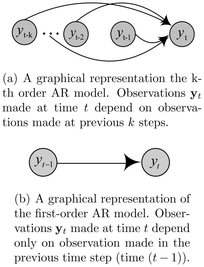
The Autoregressive Model (AR) is the most common approach for modeling time series [4]. Let y_t denote a d × 1 dimensional vector of observations made at time t, and y_t−i a d × 1 dimensional vector of past observations made at time t − i. The AR(k) represents a stochastic process defining sequences of observations in terms of a transition probability distribution p(y_t|y_t−1, y_t−2, …, y_t−k) that reflects how observations at current time t depend on observations y_t−1, y_t−2, …, y_t−k made in previous k steps. The dependency among observations is linear and defined by the following equation:

$${\mathbf{y}}_t=\sum _{i=1}^k{\mathit{\phi }}_i{\mathbf{y}}_{t-i}+{\mathit{\epsilon }}_t$$ (1)

where influences of past observations on y_t at time t are parameterized using d × d transition matrices φ_i, one for each observation vector y_t−i. New observations made at time t are corrupted by a zero-mean independent-variant Gaussian noise ε_t ~ (0, σI). Figure 1(a) illustrates an AR(k) process and its special case, a one-step AR process, AR(1), is shown in Figure 1(b).

Figure 1.

Graphical representation of the k-th and the first order AR models.

AR learning and prediction

Autoregressive models are remarkably flexible at handling a wide range of different time series patterns [5, 6]. One advantage of the AR model is that the optimization of its parameters from past time series data can be formulated by solving a system of linear equations [7, 8]. Finally, the prediction for future time points based on AR corresponds to the application of eq.(1), that is, knowing the values of y₁, y₂, …, y_T up to some time T we can predict the values y_T+1, y_T+2, y_T+3 and so on, for all future times following time T.

2.2. Linear dynamical system

The LDS is a real-valued time series model that represents observation sequences indirectly with the help of hidden states. Let {z_t}, {y_t} define sequences of hidden states and observations respectively. The LDS models the dynamics of these sequences in terms of the state transition probability p(z_t|z_t−1), and state-observation probability p(y_t|z_t). These probabilities are modeled using the following equations:

$${\mathbf{z}}_t=A{\mathbf{z}}_{t-1}+{\mathbf{e}}_t;{\mathbf{y}}_t=C{\mathbf{z}}_t+{\mathbf{v}}_t,$$ (2)

where y_t is a d × 1 observation vector made at (current time) t, and z_t an l × 1 hidden states vector. The transitions among the current and previous hidden states are linear and captured in terms of an l × l transition matrix A. The stochastic component of the transition, e_t, is modeled by a zero-mean Gaussian noise e_t ~ (0, Q) with an l × 1 zero mean and an l × l covariance matrix Q. The observations sequence is derived from the hidden states sequence. The dependencies in between the two are linear and modeled using a d × l emission matrix C. A zero mean Gaussian noise v_t ~ (0, R) models the stochastic relation in between the states and observation. In addition to A, C, Q, R, the LDS is defined by the initial state distribution for z₁ with mean π₁ and covariance matrix V₁, z₁ ~ (π₁, V₁). The complete set of the LDS parameters is Λ = {A, C, Q, R, π₁, V₁}. Notice that if l = 1, LDS reduces to an AR(1) model defined in Section 2.1.

LDS learning

The parameters of the LDS model can be learned using either the Expectation-Maximization (EM) algorithm [9] or spectral learning algorithms [10, 11]. The EM algorithm iteratively finds the distribution over hidden states that maximize the likelihood of the observed data. Spectral approaches like Ho-Kalman SSID² [12], N4SID³ [10] provide a non-iterative, asymptotically unbiased solution in closed form. Due to iterative reestimation the EM is slower than spectral methods that do not iterate. However, the EM tends to perform better than spectral methods when the number of examples available to train the model is small.

LDS prediction

The predictions for future time points based on LDS involve two steps: inferring the hidden states and making predictions. The first step can be accomplished with Kalman Filtering algorithm [1] that for observed values of y₁, y₂, … y_T up to some time T infers hidden state z_T. In the second step, by applying eq.(2), we can get predicted hidden state value z_T+1, z_T+2, z_T+3 …, and therefore, we can predict the values y_T+1, y_T+2, y_T+3 and so on, for all future times following time T.

Comparing AR and LDS model, the observations in the AR model directly depend on previous observations, which makes the model more sensitive to noisy observations and outliers. In contrast to AR, the LDS represents the dynamics indirectly using hidden states which gives one additional flexibility to better capture the different modes the system may exhibit and is more robust when observations are noisy. A drawback of the AR, is to decide how many past observations are needed to model the dynamics. Similarly, the quality of the LDS depends on the number of hidden states one uses to model observation sequences.

2.3. Gaussian process model

The GP is a popular nonparametric nonlinear Bayesian model in statistical machine learning. A GP is a collection of random variables, any finite number of which have a joint Gaussian distribution. The GP is best viewed as an extension of the multivariate Gaussian to infinite-sized collections of real-valued variables defining the distribution over random functions. Table 1 summarizes the relationship between Gaussian distribution, multivariate Gaussian distribution and the GP.

Table 1.

Relationship between Gaussian distribution, multivariate Gaussian distribution and Gaussian process.

	Mean Type	(Co)variance Type
Gaussian distribution	scalar	scalar
multivariate Gaussian distribution	vector	matrix
Gaussian process	function	function

A GP is represented by the mean function m(x) = [f(x)] and the covariance function K(x, x′) = [(f(x) − m(x))(f(x′) − m(x′))], where f(x) is a real-valued process and x is the input vector. The mean function m(x) indicates the central tendency of the process and the covariance function controls the variation in terms of the similarity or distance of the two input vectors x and x′.

The GP can be used to calculate the distribution p(f(X^*)) of f values for an arbitrary set of inputs X^*. The distribution is a multivariate Gaussian p(f(X^*)) = (m(X^*), K(X^*, X^*)). It defines the prior distribution of f(X^*). In addition, the GP can be used to calculate the posterior distribution p(f(X^*)|(X, Y)) of f values for inputs X^*, given a set of observed values Y for X, where Y = f(X) + ε, assuming additive independent identically distributed Gaussian noise ε with variance σ², ε ~ (0, σ²). The posterior is again a multivariate Gaussian p(f(X^*)|(X, Y)) = (m(X^*|(X, Y)), Cov(X^*|(X, Y))) where the mean and covariance expressions are:

$$m(X^{\ast }\mid (X,Y))=m(X^{\ast })+K(X^{\ast },X){[K(X,X)+{\sigma }^{2}I]}^{-1}(Y-m(X))$$ (3)

$$\mathit{Cov}(X^{\ast }\mid (X,Y))=K(X^{\ast },X^{\ast })-K(X^{\ast },X){[K(X,X)+{\sigma }^{2}I]}^{-1}K(X,X^{\ast }).$$ (4)

Figure 3 illustrates the examples of functions drawn from the GP prior and posterior in a 1-D space; Figure 3(a) shows functions drawn from the prior distribution function values at X^*. Figure 3(b) shows functions drawn from the posterior distributions given that some data points (X, Y) are observed.

Figure 3.

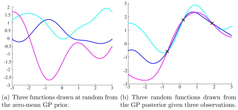
Graphical illustration of GP prior and posterior. In this example, we create X^* as a linearly spaced vector from −3 to 3 with step size 0.01. We set the mean function m(·) = 0 and covariance function K(x, x′) = exp(−(x − x′)²/2).

The GP methodology can be applied to time series modeling problem by representing observations as a function of time. As a result, there is no restriction on when the observations are made and whether they are regularly or irregularly spaced in time.

The parameters of the GP are formed by parameters defining the mean and covariance functions. Typically, the covariance function makes sure the function values for two nearby times tend to have high covariance, while values from inputs that are far apart in time tend to have a low covariance. The parameters can be learned from data that consist of one or many examples of time series. The predictions of values at future times correspond to calculation of posterior distribution for these times.

In summary, the advantage of the GP model is that it lets us represent the functions of time. A disadvantage is that one has to apriori pick and parameterize the mean and covariance functions, and the mean function must be a function of time.

3. Modeling clinical time series

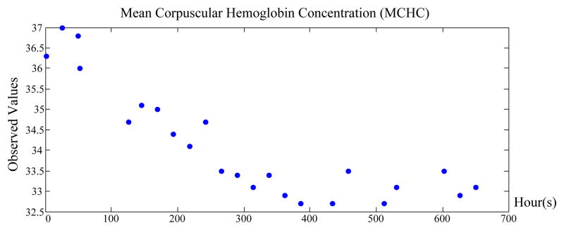
The focus of our work is on the development of time series models that are able to represent and learn as accurately as possible the dynamics of clinical time series from data. The key distinguishing feature of clinical time series corresponding to lab tests is that they are collected irregularly in time and that the time series may be sparse, that is, values may not be obtained for longer periods of time. The primary reason for this is the cost of the lab test, hence the lab orders and their frequencies strongly depend on the patient’s health condition. Figure 4 illustrates time series of Mean Corpuscular Hemoglobin Concentration (MCHC) lab results for one of the patients in our database.

Figure 4.

An example of an irregularly sampled Mean Corpuscular Hemoglobin Concentration (MCHC) data. X-axis shows time in hours since the admission of the patient.

The presence of irregularly sampled data prevents us from directly applying the discrete time models reviewed earlier, since both the AR and LDS assume a fixed sampling frequency that defines a unit of time. Hence the challenge is to modify the existing or devise new time series models that can deal better with changes in data collection times. In the following, we show different ways of modifying the existing time series approaches to achieve this goal. However, prior to presenting these methods we discuss the criteria we use to judge the quality of these models.

While many different ways of measuring the quality of the time series models can be devised, in this work, we judge the model quality in terms of its ability to predict the values of future clinical observations for a patient given his/her past clinical data. More formally, we judge the models by considering the quality of the time series prediction/regression function:

$$g:{\mathbf{Y}}_{\text{obs}}\times t\to {\widehat{\mathbf{y}}}_t$$ (5)

where Y_obs is a sequence of past observation-time pairs ${\mathbf{Y}}_{\text{obs}}={({\mathbf{y}}_i,t_i)}_{i=1}^n$, such that, n is the number of past observations, 0 < t_i < t_i+1, and y_i is a d-dimensional observation vector made at time (t_i). Time t, t > t_n, is the time at which we would like to predict the future observation ŷ_t. This prediction problem is also illustrated in Figure 5. Please note that in our formulation of the prediction problem (eq.(5)), times of the different observations may vary, reflecting the data collection irregularities. In general, the labs are collected at the different times of the day and the observed sequences may be sparse.

Figure 5.

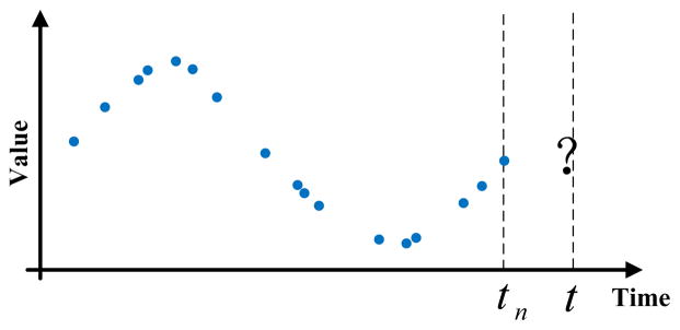
Prediction problem for an irregularly sampled time series data. Blue dots denote past observations already made for the patient. The question mark denotes future time points we want to predict.

3.1. Modeling clinical data with discrete time models

In general, there are two ways to handle irregularly sampled time series datasets and convert them to observation sequences one can model and analyze using the discrete time models: (1) direct value interpolation (DVI) approach; and, (2) window-based segmentation (WbS) approach. In the following we briefly summarize these two approaches.

3.1.1. Direct value interpolation approach

The DVI approach assumes that all observations are collected regularly with a pre-specified sampling frequency R. However, instead of actual readings the values at these time points are estimated from readings at time points closest to them using various interpolation techniques [13–18]. The interpolated (regular) time series are then used to train a discrete time model (either AR or LDS). The approach is illustrated in Figure 6. In terms of predictions of future values, one has to first use trained discrete time model to predict the values at time points closest to the target time, and after that, apply the interpolation approach to estimate the target value.

Figure 6.

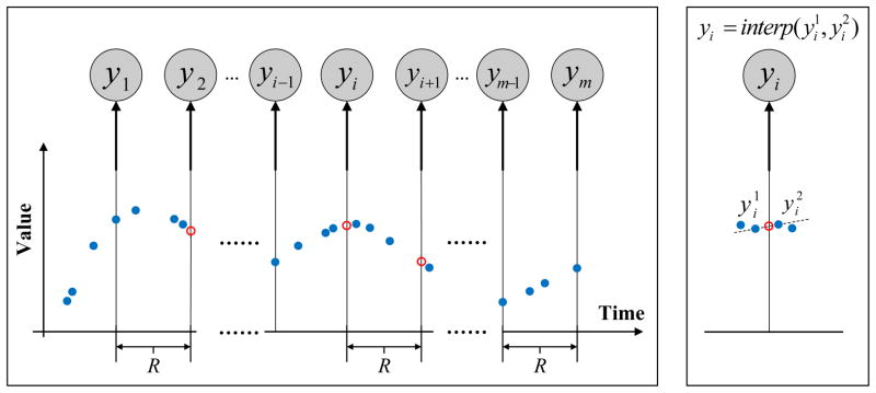
Transformation of irregularly sampled time series to a discrete time series by DVI. The red circles denote the interpolated values with no readings. The right panel illustrates the linear interpolation process.

The DVI approach converts the time series with irregular observations to discrete time observation sequences. The quality of the conversion depends on the number of observations actually seen and the sampling frequency parameter R. One straightforward way to set R is to use internal cross-validation approach. Briefly, we divide the time series data used for training the models to folds and use them to built multiple internal training and testing datasets. The models built with different sampling frequencies R are tested on the internal test sets, and the best R that leads to the best prediction accuracy on the internal test data (averaged over different folds) is selected.

3.1.2. Window-based segmentation approach

The WbS approach is slightly different. Instead of values at pre-specified regularly sampled time points, the approach first segments time series to fixed-sized windows. The behavior in the window is summarized in terms of its statistics γ, such as, the mean, or the last value observed within that time interval [19–24]. The values generated by the different windows define sequences of γ statistics. The discrete time model (AR or LDS) is then used to represent how the summary statistics γ in two consecutive windows change, that is, a sequence of statistics calculated over these intervals are considered to be observations of the discrete time model. Predictions at future times for the window-based approach are made using the discrete time model by identifying the time interval the target time point falls into.

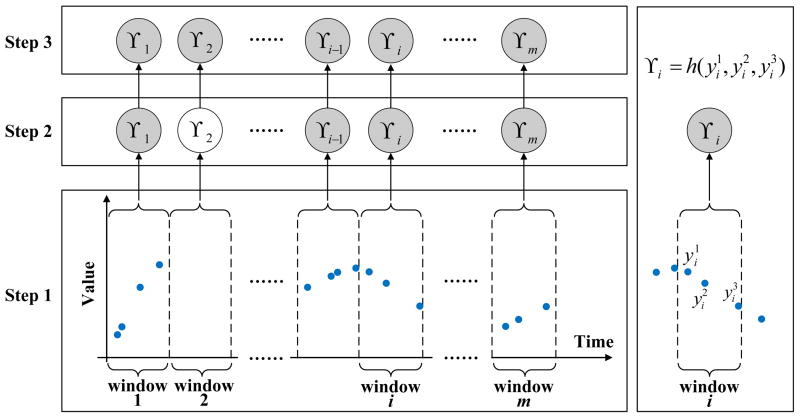
We would like to note that in order to learn the parameters of the window-based discrete time model from irregularly sampled data one has to either assure that every time interval has at least one reading that is sufficient to calculate the summary statistics; or impute the statistics for the window with missing values from its neighbors using, for example, interpolation methods. In this work, we implement the window-based approach that relies on interpolations to fill statistics in intervals with missing values. Figure 7 illustrates the process. Briefly, after segmentation of time series to windows of a fixed size (step 1), the summary statistics γ_i for each window i are calculated (step 2), and for windows with no readings, the statistics are interpolated from windows next to it (step 3). Once the missing statistics are imputed, the AR or the LDS models can be learned from complete sequences γ₁, γ₂, ···, γ_m of summary statistics derived from time series of labs for multiple patients. The algorithms for learning the AR and LDS models were reviewed in Section 2.1 and Section 2.2.

Figure 7.

Transformation of irregularly sampled time series to a discrete time series by WbS. The shaded nodes denote summary statistics calculated from the corresponding windows, such as γ₁, γ_i in Step 2. The regular (unshaded) nodes denote empty summary statistics corresponding to windows with no readings, such as γ_2. h in the right panel denotes the summary statistics estimation function.

The AR and LDS models (once they are learned) can be used for prediction by taking an initial sequence of lab observations for a new patient and predicting lab values at an arbitrary future time t. This is accomplished by first applying the WbS to observed data for the new patient and by calculating or imputing the statistics γ for each window. The value at some future time t is predicted by using the time series model (AR or LDS) to predict the statistics γ^* for the window the future time falls into and after that infer the value for target time t from γ^*. We note the simplest implementation of step 3 is to predict the value directly with the summary statistic. Briefly, if the summary statistic reflects the value of observations in the respective time window, we may directly use this value to predict the lab value for any time that falls within the corresponding window.

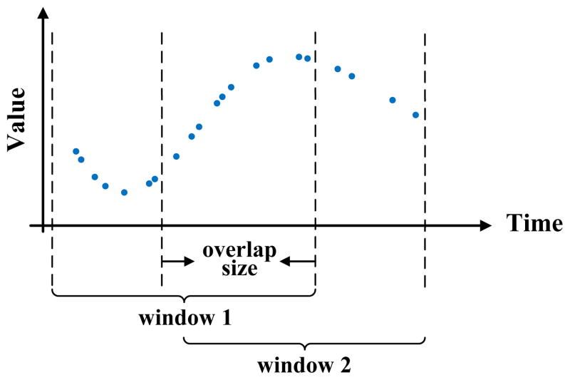
The above window-based approach can be further refined by overlapping two consecutive windows that generate the statistic γ in time. This means some of the observations can be shared by two windows and may influence the statistics in two consecutive steps. Overlapping the two windows helps to smooth the transitions in statistics. In addition, it helps to generate longer sequences one can use to train better models. The idea of window overlap is illustrated in Figure 8. Considering windows and their overlaps, the segmentation of the time series is induced by two parameters: the window size and the overlap size . These are additional parameters of the WbS approach, and if needed, they can be optimized using the internal cross-validation approach. Details are discussed in Section 5.4.

Figure 8.

Graphical illustration of WbS with overlaps on the irregularly sampled time series data.

3.1.3. Advantages and limitations of discrete time models

The advantage of the above discrete time models is their relative simplicity. The learning and prediction procedures are intuitive and well developed. The disadvantages of the models are: (1) AR and LDS are linear models. The linearity may prevent them from modeling more complex time series data. (2) AR and LDS are discrete models, both learning and prediction are restricted to either the fixed time points or fixed time windows which may introduce additional errors when modeling observations made at arbitrary times.

3.2. Modeling clinical data with a continuous time GP model

The GP reviewed in Section 2.3 lets us define the distribution over functions and hence can model sequential observations as a function of time. This appears to be promising when the time series is hard to discretize in time as is the case with clinical time series data in which observations are often missing and spaced irregularly in time.

As mentioned in Section 2.3, the GP is parametrized by its mean function and covariance function, where the mean function is the function of time. The question now is how to pick the mean and covariance functions that work well with clinical time series data.

Mean function

The mean function of the GP is a function of time. We want to learn a function that fits many patients and their clinical time series. Since the patients may be encountered at different age and under different circumstances, there is no good way to align their time origins. Hence the only way to feasibly align them is to set their mean functions equal to a constant m(t) = M, which makes the mean function of a GP time invariant.

Covariance function

The covariance function measures the similarity of two function values f(t) and f(t′) based on their input time t and t′. In general, the covariance function should reflect the properties of the modeled time series, such as its smoothness or periodicity. In order to model covariances of clinical time series for numerical labs we make the following assumptions: the readings made at times t and t′ which are close are likely to have similar reading values f(t) and f(t′), and the readings very close in time may change more abruptly. To represent these assumptions we choose and combine two covariance function models: the Gaussian kernel eq.(7)) and the mean reverting kernel eq.(6):

$$K(t,t^{\prime })={\sigma }_{1}exp({\alpha }_1\mid t-t^{\prime }\mid )$$ (6)

$$K(t,t^{\prime })={\sigma }_{2}exp({\alpha }_2{(t-t^{\prime })}^2)$$ (7)

The Gaussian kernel is the most frequently used kernel in literature [25–27] that promotes smoothness and pushes two different readings closer when they are close in time. The second kernel represents the mean reverting process and while it forces the two readings close in time to be similar, it also permits more abrupt changes in their observed values [2, Chapter 4]. To approximate the clinical time series we use a linear combination of eq.(6) and eq.(7) together with the observational noise component ε ~ (0, σ²) (See Section 2.3) as our covariance function:

$$K(t,t^{\prime })={\sigma }_{1}exp({\alpha }_1\mid t-t^{\prime }\mid )+{\sigma }_{2}exp({\alpha }_2{(t-t^{\prime })}^2)+{\sigma }^2{\delta }_{t,t^{\prime }}.$$ (8)

In this model, Θ = {σ₁, α₁, σ₂, α₂, σ} are parameters of the covariance function that can be learned directly from data. δ_t,t′ is a Kronecker delta which is one iff t = t′ and zero otherwise.

3.2.1. Learning the GP model

As discussed in the previous section, we set the mean function to a constant M to ensure its time invariant property. To obtain M, we can average all the observations from all the patients and use that averaged value as the constant M for the mean function. This gives us a constant mean which reflects many patients and their clinical time series.

To learn the parameters of the covariance function, we seek Θ that can maximize the marginal likelihood p(Y|X) [2]. The log marginal likelihood for GP is shown in eq.(9).

$$logp(\mathbf{Y}\mid X)=-\frac{1}{2}{\mathbf{Y}}^{\top }{K}_{\mathbf{Y}}^{-1}\mathbf{Y}-\frac{1}{2}log\mid K_{\mathbf{Y}}\mid -\frac{n}{2}log2\pi$$ (9)

where Y denotes all the training observations. K_Y = K + σ²I is the covariance matrix for the noisy observations Y and K is the covariance matrix for noisy-free function values from function f, Y = f(X) + ε, ε ~ (0, σ). n is the number of observations.

The partial derivatives of the marginal likelihood with respect to each parameter θ_i in Θ is shown in eq.(10).

$$\frac{\partial }{\partial {\theta }_i}logp(\mathbf{Y}\mid X,\mathrm{\Theta })=-\frac{1}{2}\text{Tr}\left[K_{\mathbf{Y}}^{-1}\frac{\partial K_{\mathbf{Y}}}{\partial {\theta }_i}\right]+\frac{1}{2}{\mathbf{Y}}^{\top }{K}_{\mathbf{Y}}^{-1}\frac{\partial K_{\mathbf{Y}}}{\partial {\theta }_i}{K}_{\mathbf{Y}}^{-1}\mathbf{Y}$$ (10)

where Θ represents the entire set of parameters in covariance function, θ_i ∈ Θ = {σ₁, α₁, σ₂, α₂, σ}. Tr is the trace operator.

Once we have the partial derivatives with respect to each parameter, any well developed gradient based methods can be directly applied to maximize p(Y|X).

3.2.2. Predicting with GP model

Since GP is a function of time, it can be easily applied to make future time prediction. Given any time index t we can calculate its posterior mean with eq.(3), and use it to predict the values at that time. Figure 9 illustrates this step.

Figure 9.

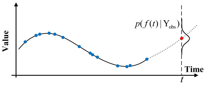
Graphical illustration of the prediction problem on a GP model on irregularly sampled time series data. The solid line denotes the GP we learned from the data and the dotted line indicates the GP’s predictions of future values for future time t. The posterior distribution of f(t) at time t is shown and the red dot is the mean of that distribution, which is the value predicted by the GP.

3.2.3. Advantages and limitations

Continuous time models, like GP, define a continuous time process, as opposed to discrete time models such as AR or LDS. This appears to be promising especially when the problem is hard to discretize in time and particularly useful for our problem in which observations are spaced irregularly in time.

Unfortunately, this approach also comes with limitations; the most serious one is that the mean function of the GP is a function of time and in order to make the GP independent of the time origin we need to set it to a constant value. However, this significantly limits our ability to represent changes or different modes in time series dynamics.

4. Hierarchical dynamical system framework

While AR, LDS and GP models can be adapted to model irregularly sampled clinical time series data they also come with drawbacks that may limit their performance. More specifically, discrete time models are not able to represent well sequences of lab values in real time because values need to be re-estimated from quantities with a discrete time step. On the other hand, a continuous time GP model with a constant mean function is too restrictive and cannot model the different modes of dynamics or different subpopulations of patients well. On the positive side, discrete time models, especially LDS, are good at modeling changes in both the dynamics and different modes in time series behavior, while GP models are good at modeling time series in real time. Considering the respective advantages and limitations of the two frameworks, a combination of the two appears as the best solution to offset their limitations.

4.1. The model

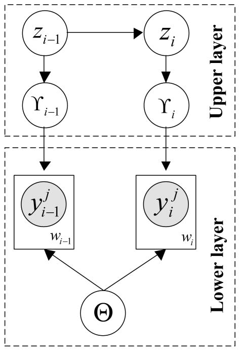
To follow the above intuition, we propose a new hierarchical dynamical system model that splits the process into a sequence of dependent local GPs that are combined with LDS to better capture higher-level changes in the time series dynamics. The local GPs’ dependencies naturally account for the transitions of mean functions and irregular samples are handled by the local GPs themselves.

The structure of our model is shown in Figure 10. Briefly, the model consists of two hierarchically related processes: a Gaussian process and a linear dynamical system. The GP is restricted to a time window of finite duration and is used to represent a time series and its dynamics for shorter time spans. Longer-term process changes are modeled and controlled by the LDS. In the lower layer, which is shown using a dashed line box, we map the entire irregular time series data into m windows w_is, i = 1, …, m using the Wbs approach. Each window w_i (see Figure 10) relates observations { $y_i^1,y_i^2,\dots ,y_i^{N_i}$} using the same window-specific GP_i, where N_i is the number of observations in window w_i. Hence, instead of using a single GP, we capture a time series by using many different window-specific local GPs and model global changes in dynamics using the upper level LDS that controls the means of the window specific GPs.

Figure 10.

Graphical illustration of our hierarchical dynamical model combining the GP and the LDS. The shaded nodes denote irregular observations. The γ node is the window representative we extract from the corresponding window and the z node is the hidden state we introduce in LDS to model the change of γs. The Θ node represents the shared covariance function parameters for all the GPs.

That is, the LDS represents the dynamics and changes of summary statistics γ_is defining individual GP_is. The upper level LDS is defined as:

$${\mathbf{z}}_i=A{\mathbf{z}}_{i-1}+{\mathbf{e}}_i;{\gamma }_i=C{\mathbf{z}}_i+{\mathbf{v}}_i$$ (11)

where summary statistics γ_is act like observations, and e_i and v_i are zero-mean normally distributed random variables with covariance matrices Q and R respectively. Similarly to regular LDS introduced in Section 2.2, π₁ and V₁ are the initial state mean and variance.

4.2. Learning

We learn the parameters of our hierarchical dynamical model by devising solutions to two estimation/learning problems: (1) learning of the parameters Θ of the covariance function defining the lower level GPs, and (2) learning of the parameters of the upper level LDS.

Estimation of the covariance function

Since all window-specific GP_is share the same covariance function, we set Θ by maximizing the like-lihood using the partial derivative of the likelihood with respect to each parameter θ_i in Θ as defined in eq.(10).

Estimation of the LDS parameters

The LDS controls the means of individual window-specific GPs. We learn its parameters as follows:

• Step 1. Use WbS approach to estimate summary statistics γ_is from observations in windows w_is. The γ_is represent the means of window-specific GP_is. In general, there are many different ways to estimate γ_is. Let h denote a function used for estimating the mean of the GP from observations { $y_i^1,y_i^2,\dots ,y_i^{N_i}$}. Examples of h can be max, mean or last functions that return the maximum, the mean, or last observed value in the window. In this work, we use the mean function as the estimator of window-specific GP means.

• Step 2. Use sequences of γ statistics as observations of the upper level LDS in our hierarchical dynamical system. To learn the parameters of the LDS, we use the EM learning algorithm to iteratively re-estimate the parameters Λ = {A, C, Q, R, π₁, V₁} defining the LDS [9], similarly to standard LDS learning.

4.3. Prediction

Once the hierarchical dynamical system is learned from the training data we would like to use it to support predictions on future time series. Given the initial observations Y_obs and an arbitrary future time t, the value y_t is predicted as follows:

• Step 1. Split Y_obs into windows and continue splitting time after Y_obs into windows until one contains t. The index of the window containing t is λ and the index of the window containing the last observation in Y_obs is τ.

• Step 2. Estimate summary statistics γ_is for all windows up to window τ using Y_obs using the WbS approach. After that use these statistics to predict γ_λ with the upper level LDS system.

• Step 3. Compute the value ŷ_t at future time t using the posterior mean of the GP with the mean function γ_λ, covariance parameters Θ and past observations Y_obs

5. Experiments

5.1. Data description

We have tested our new approach on time series data obtained from electronic health records of 4,486 post-surgical cardiac patients stored in PCP database [28–31]. To test the performance of our prediction model, we have randomly selected 1000 patients that had at least 10 CBC tests ordered during their hospitalization. We used ten tests from the CBC panel to learn ten different time series models, and evaluated them on the time series prediction task. The ten tests, their means and standard deviations, are listed below:

• White blood cell (WBC) is a count of the total number of white blood cells in a person’s sample of blood. The number of white blood cells give important information about the immune system. Mean: 11.9778(×10⁹/L); standard deviation: 6.0826.

• Hematocrit (HCT) measures the amount of space (volume) red blood cells take up in the blood. The value is given as a percentage of red blood cells in a volume of blood. Mean: 28.6673(%); standard deviation: 4.7253.

• Hemoglobin (HGB) measures the amount of hemoglobin in blood and is a good measure of the blood’s ability to carry oxygen throughout the body. Mean: 9.5923(g/dL); standard deviation: 1.6660.

• Mean corpuscular hemoglobin concentration (MCHC) is a calculation of the average concentration of hemoglobin inside a red cell. Mean: 33.8588(g/dL); standard deviation: 0.8112.

• Mean corpuscular hemoglobin (MCH) is a calculation of the average amount of oxygen-carrying hemoglobin inside a red blood cell. Mean: 30.5371(pg/cell); standard deviation: 1.7567.

• Mean corpuscular volume (MCV) is a measurement of the average size of patient’s red blood cell. Mean: 90.1673(fL); standard deviation: 4.5538.

• Mean platelet volume (MPV) Mean platelet volume measures the average amount (volume) of platelets. Mean platelet volume is used along with platelet count to diagnose some diseases. Mean: 8.7310(fL); standard deviation: 1.1834.

• Platelet (PLT) count is the number of platelets in a given volume of blood. Platelets are important in blood clotting. Mean: 202.0661(×10⁹/L); standard deviation: 126.7321.

• Red blood cell (RBC) is a count of red blood cells carry oxygen from the lungs to the rest of the body. Red blood cells also carry carbon dioxide back to the lungs so it can be exhaled. Mean: 3.2137(×10¹²/L); standard deviation: 0.5610.

• Red cell distribution width (RDW) is a calculation of the variation in the size of red blood cells. It shows if the cells are all the same or different sizes or shapes. Mean: 16.7745(%); standard deviation: 2.6424.

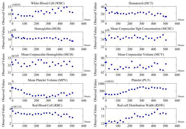
These time series data are noisy; their signals fluctuate in time, and the time periods between observations vary. Figure 11 illustrates such a time series for one of the patients. The X-axis is the time index aligned by hour and the Y-axis are normalized values/observations for each test.

Figure 11.

Time series for ten tests from the CBC panel for one of the patients.

5.2. Baseline methods

We compare our two-layer hierarchical dynamical system approach with LDS and GP layers (HDSGL) to six baseline methods:

1. First-order autoregressive (AR) process trained on the entire time series using DVI approach. We applied linear interpolation directly to fill the missing values.

2. Linear dynamical system (LDS) trained on the entire time series using DVI approach. We applied linear interpolation directly to fill the missing values.

3. Standard Gaussian process regression (GP) with constant mean function. The choice of covariance function is the linear combination of eq.(6) and eq.(7).

4. Window-based AR (WAR). Irregular sampled time series is handled by WbS, as described in Section 3.1. It splits the time series first into windows and, after that, it trains an AR over the windows’ summary statistics.

5. Window-based LDS (WLDS). Irregularly sampled time series is handled by WbS, as described in Section 3.1. It splits the time series first into windows and, after that, it trains an LDS over the windows’ summary statistics.

6. Hierarchical dynamical system combined with GP and AR process (HDSGA). HDSGA is similar to HDSGL, but we change the upper layer LDS to the first order AR process.

We set the summary statistics estimation function h that is used to calculate the summary statistics γ_i for each window i for all WbS approaches (WAR, WLDS, HDSGA and HDSGL) to the mean of the values observed in that window. Also, we use the combination of the mean reverting and the diagonal squared exponential functions as the covariance function for all GP related methods (GP, HDSGA, HDSGL) as was discussed in Section 3.2.

5.3. Experiment settings

To evaluate the performance of our hierarchical dynamical system approach we randomly divided patients and their time series into the training and testing sets, such that data for 200 patients form the test data and time series data for 800 patients were used for training.

Evaluation metric

Our objective is to test the predictive performance of our approach by its ability to predict the future value of an observation for a patient for some future time t given a sequence of patient’s past observations. We judged the quality of the prediction using the Mean Absolute Error (MAE) on multiple test data predictions. Instead of Root Mean Square Error (RMSE), which gives a relatively high weight to large errors (the errors are squared before they are averaged), MAE is the average over the absolute values of the differences between predictions and the corresponding observations. The MAE is a linear score which means that all the individual differences are weighted equally in the average. More specifically, the MAE is defined as follows:

$$\mathit{MAE}=\left[n^{-1}\sum _{i=1}^n\mid y_i-{\widehat{y}}_i\mid \right]$$ (12)

where y_i is the true value, ŷ_i is the predicted value and n is the number of prediction tasks attempted.

To conduct the evaluation, we use the test dataset to generate various prediction tasks as follows. For each patient i and complete time series for that patient, we calculate the number of observations n_i in that time series. We use n_i to generate all different pairs of indices (ψ, ϕ) for that patient, such that 1 ≤ ψ < ϕ ≤ n_i, where ψ is the index of the last observation assumed to be seen, and ϕ is the index of the observation we would like to predict. By adding time stamp reading to each index, the two indices help us define all possible prediction tasks, we can formulate on that time series. Let Γ_i be the total number of different indices pairs (or Γ_i different prediction tasks) for patient i and ${\sum }_{i=1}^{200}{\mathrm{\Gamma }}_i$ is total number of prediction tasks in our test data. For each method, we use the MAE on these tasks to judge the quality of test predictions and run the pair-wise t-test on the ${\sum }_{i=1}^{200}{\mathrm{\Gamma }}_i$ prediction tasks’ results from our method and all the other baselines to check the statistical differences between them. In addition, we use the bootstrap approach [32] to compute the 95% the confidence interval on MAE for each method.

5.4. Settings of window parameters

All methods, but the GP that is applied directly to observed data, rely on some discretization of time to reflect either the sampling frequency for the DVI or the window and overlap sizes for the WbS. These define additional parameters our methods depend on and that need to be optimized. To optimize them we use the internal cross-validation approach. Briefly, we split 800 time series in the training data using four-fold cross-validation into four 600:200 internal training and testing datasets. We vary the window size parameter for every fold by checking values {1, 2, 3, 4, 5, 6, 7} days and the overlap size using {0, 1, 2, 3, 4, 5, 6} days and pick the parameters that achieve the best average performance across all four folds. The parameters are optimized independently for each method tested. For the DVI approaches we optimize the sampling frequency parameter R using the same internal four-fold cross-validation approach. We vary the sampling frequency parameter for every fold by checking values {1, 4, 6, 8, 12, 24} hours.

5.5. Results

5.5.1. Overall prediction performance

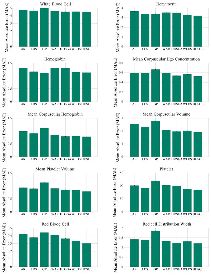
In the overall prediction experiment, we follow the procedure described in Section 5.3 to generate and randomly select different prediction tasks. These contains both short-term and long-term predictions depending on the difference in between the time at which we predict the value and the time of the last observation seen. Figure 12 shows the results of the prediction experiment for all methods. (Detailed numerical results are shown in Table 2 in Appendix.) The result shows the mean MAE for each method.

Figure 12.

MAE on CBC test samples for random prediction tasks.

The results of our experiments (Figure 12 and Table 2) show that our hierarchical dynamical system (HDSGL) outperforms all other methods in terms of prediction error on the CBC test data. The results are statistically significantly different at 0.05 level for all labs. We determined the significance by running the pairwise t-test comparing the HDSGL to all other methods on all corresponding prediction tasks.

We believe the main reason for the hierarchical approach outperforming all other methods is that it directly models and works with real time series (via lower level GP) and that it minimizes the effect of noisy observations by using window-based summary statistics. The hidden states of the upper layer LDS are able to capture the change of those summary statistics. The lower layer GP can adjust the prediction values based on the mean of the upper layer and the few observations we have, which gives us the lowest MAE.

Furthermore, by comparing methods with hidden states (HDSGL, WLDS, LDS) to methods without hidden states (AR, GP, WAR, HDSGA), we can see that methods involving hidden states are more accurate than methods that model the dynamics using only observations. We believe that hidden states increase the hidden state models’ ability to capture the complexity of the time series, and that methods directly learned from observations are more sensitive to the observation noise, which is quite common in real clinical time series datasets.

5.5.2. Short-term prediction performance

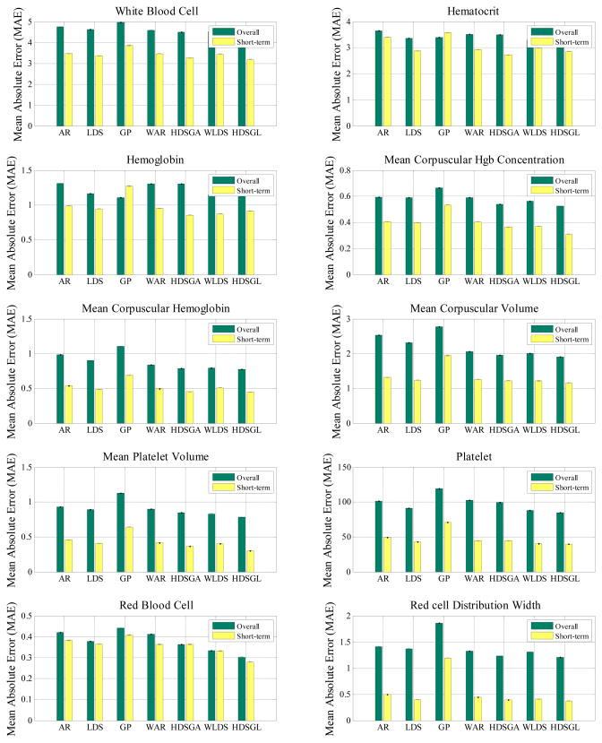
The above experiment randomly selects from among many different prediction tasks. These may include both short-term and long-term predictions depending on the difference in between the time at which we predict the value and the time of the last observation seen. We expect that short-term predictions that are close to the last value observed should be better. To verify this expectation, we conduct a new experiment where observation indices for the prediction tasks involve (ψ, ϕ) pairs that satisfy ϕ = ψ +1, that is, we always try to predict the next lab reading. Figure 13 compares our method and the baselines in terms of their corresponding overall and short term prediction performances. Detailed numerical results for short-term prediction are shown in Table 3 in Appendix.

Figure 13.

MAE on CBC test samples for the random and short-term prediction tasks.

As we can see from Figure 13, for all lab tests, short-term predictions are much better than overall predictions (that include both short and long term prediction), which supports our intuition that the further we predict, the worse predictions we make. In addition, we see our method remains the best in all the lab tests for the short term prediction tasks.

5.5.3. Performance summary

In order to summarize the predictive performance of our algorithm and its benefits, we compute, for each CBC lab test, the relative prediction error improvement against the best alternative method in both overall prediction and short-term prediction tasks. More specifically, we compute the relative prediction error improvement percentage by calculating the MAE difference between the best baseline method and our algorithm and then dividing the difference by the best baseline error. By averaging the relative prediction error improvements over all CBC labs, our method achieved a 3.13% average prediction accuracy improvement on ten CBC lab time series in the overall prediction tasks and a 5.25% average prediction accuracy improvement in the short-term prediction tasks.

5.6. Clinical expert evaluation

In Section 5.5, we compare our hierarchical model HDSGL with different baselines using MAE and show that our model performs better in both overall prediction and short-term prediction tasks. However, it is not clear whether the predictions made by our model are clinically acceptable or not. In order to assess the clinical relevance of predictions, we consulted a clinical expert, and converged to the following clinical evaluation.

As the clinical expert suggests, the importance of the error should be judged relative to its value. Briefly, a deviation of prediction by 10 units for the value of 20 is significantly worse than the same deviation for the value of 100. In order to reflect this, we calculate Absolute Error Percentage (AEP) to measure the quality of each prediction task made by the HDSGL approach. AEP is defined as follows:

$$\mathit{AEP}=\frac{\mid y_i-{\widehat{y}}_i\mid }{y_i}\times 100\%$$ (13)

where y_i is the true value, ŷ_i is the predicted value. Briefly, AEP reflects how much deviation we have from our prediction to the true value.

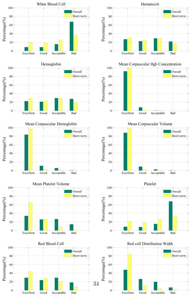
After calculating the AEP for each prediction, we categorize its result into four qualitative categories suggested by the expert:

1. Excellent. The prediction task’s AEP is less than 5%.

2. Good. The prediction task’s AEP is between 5% and 10%.

3. Acceptable. The prediction task’s AEP is between 10% and 20%.

4. Bad. The prediction task’s AEP is greater than 20%.

These four categories tell us how well the model is able to predict the lab values in terms of their clinical acceptance. We use these four categories to calculate the distribution of predictions for each lab test in terms of both overall (Section 5.5.1) and short-term predictions (Section 5.5.2). Figure 14 summarizes the distributions of these qualitative prediction categories for all ten lab tests. (Detailed numerical results are shown in Table 4 and Table 5 in Appendix.)

Figure 14.

Clinical evaluations of HDSGL for both overall prediction and short-term prediction quality distributions.

Discussion

In terms of clinical acceptance, we see that the results differ widely for the different labs. In particular, very good short and long term predictions are achieved for CBC lab components that are less sensitive to blood loss and drip infusions that are rather frequent during the management of post-surgical cardiac patients. These labs include: MCHC, MCH, MCV, MPV and RDW.

On the other hand, WBC, RBC, HCT, HGB and PLT labs are measured relative to the blood volume and hence are sensitive to the above events. Consequently the prediction quality of these models goes down. Overall, the results for these labs suggest the predictions based only on previous sequences of lab values alone may not be sufficient, and additional variables representing the different future events and/or possible patient management steps should be included in the model to improve its prediction quality.

6. Conclusion

In this work, we have presented a new two-layer hierarchical dynamical system model for time series prediction. Compared to traditional LDSs and modern GP regression, the new system adapts better to irregular sampling and it is more accurate when making predictions for different future times. Experimental results on real world clinical data from electronic health records systems demonstrate that our prediction model leads to errors that are statistically significantly lower than errors of other state-of-the-art approaches.

The limitation of the presented work is that it focuses on the analysis and modeling of univariate time series. In the future, we plan to extend our study to multivariate time series models reflecting the dependences among individual time series. A related open question is the dimensionality of the hidden state space that would be sufficient to accurately capture the dynamics of all these time series. Finally, we plan to study extensions of our current models to controlled dynamical models such as [33–37] that would let us incorporate the effect of external events and actions on future lab values and accuracy of their predictions.

Figure 2.

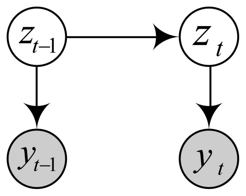
Graphical representation of the LDS. Shaded nodes y_t and y_t−1 denote observation made at current and previous time steps. Unshaded nodes z_t and z _t−1 denote the corresponding hidden states. The links represent dependences among the observations and hidden states.

Appendix

Table 2.

MAE on CBC test samples for overall prediction tasks.

Method	AR	LDS	GP	WAR	HDSGA	WLDS	HDSGL
WBC	4.7941 ± 0.0027	4.6805 ± 0.0026	5.0235 ± 0.0025	4.6400 ± 0.0026	4.5390 ± 0.0026	4.5720 ± 0.0027	4.4710 ± 0.0027
HCT	3.6893 ± 0.0007	3.3925 ± 0.0007	3.4253 ± 0.0007	3.5431 ± 0.0007	3.5315 ± 0.0007	3.3271 ± 0.0007	3.2177 ± 0.0007
HGB	1.3218 ± 0.0004	1.1755 ± 0.0004	1.1208 ± 0.0004	1.3198 ± 0.0004	1.3171 ± 0.0004	1.1577 ± 0.0004	1.1348 ± 0.0004
MCHC	0.6012 ± 0.0004	0.5959 ± 0.0004	0.6724 ± 0.0004	0.5963 ± 0.0004	0.5458 ± 0.0004	0.5701 ± 0.0004	0.5297 ± 0.0004
MCH	0.9941 ± 0.0006	0.9091 ± 0.0007	1.1154 ± 0.0007	0.8480 ± 0.0006	0.7975 ± 0.0006	0.8033 ± 0.0007	0.7831 ± 0.0007
MCV	2.5619 ± 0.0012	2.3410 ± 0.0014	2.8034 ± 0.0018	2.0814 ± 0.0012	1.9804 ± 0.0012	2.0294 ± 0.0013	1.9284 ± 0.0013
MPV	0.9412 ± 0.0005	0.9029 ± 0.0005	1.1392 ± 0.0005	0.9059 ± 0.0005	0.8554 ± 0.0005	0.8406 ± 0.0005	0.7901 ± 0.0005
PLT	102.5242 ± 0.0587	92.2360 ± 0.0561	120.4928 ± 0.0665	103.6683 ± 0.0587	100.6288 ± 0.0587	88.9408 ± 0.0555	85.8991 ± 0.0555
RBC	0.4242 ± 0.0002	0.3812 ± 0.0002	0.4453 ± 0.0002	0.4168 ± 0.0002	0.3663 ± 0.0002	0.3362 ± 0.0002	0.3059 ± 0.0002
RDW	1.4216 ± 0.0010	1.3860 ± 0.0010	1.8794 ± 0.0010	1.3427 ± 0.0010	1.2417 ± 0.0010	1.3185 ± 0.0010	1.2174 ± 0.0010

Table 3.

MAE on CBC test samples for short-term prediction tasks.

Method	AR	LDS	GP	WAR	HDSGA	WLDS	HDSGL
WBC	3.5072 ± 0.0103	3.3998 ± 0.0103	3.9007 ± 0.0111	3.4993 ± 0.0108	3.2973 ± 0.0108	3.4756 ± 0.0116	3.2170 ± 0.0116
HCT	3.4376 ± 0.0096	2.9078 ± 0.0093	3.6121 ± 0.0110	2.9608 ± 0.0087	2.7588 ± 0.0087	3.0218 ± 0.0097	2.8859 ± 0.0100
HGB	0.9972 ± 0.0021	0.9528 ± 0.0023	1.2865 ± 0.0042	0.9627 ± 0.0026	0.8617 ± 0.0026	0.8810 ± 0.0033	0.9227 ± 0.0033
MCHC	0.4098 ± 0.0010	0.4019 ± 0.0011	0.5384 ± 0.0015	0.4091 ± 0.0011	0.3687 ± 0.0011	0.3739 ± 0.0014	0.3129 ± 0.0014
MCH	0.5439 ± 0.0021	0.4911 ± 0.0021	0.6975 ± 0.0045	0.4998 ± 0.0021	0.4594 ± 0.0021	0.5148 ± 0.0042	0.4522 ± 0.0042
MCV	1.3327 ± 0.0057	1.2458 ± 0.0058	1.9629 ± 0.0125	1.2734 ± 0.0059	1.2330 ± 0.0059	1.2288 ± 0.0115	1.1729 ± 0.0115
MPV	0.4628 ± 0.0014	0.4122 ± 0.0014	0.6472 ± 0.0019	0.4213 ± 0.0014	0.3708 ± 0.0014	0.4066 ± 0.0019	0.3055 ± 0.0019
PLT	49.6031 ± 0.1156	43.4901 ± 0.1191	71.5818 ± 0.1603	45.0584 ± 0.1208	45.0584 ± 0.1208	40.8308 ± 0.1669	40.2046 ± 0.1669
RBC	0.3862 ± 0.0011	0.3685 ± 0.0011	0.4120 ± 0.0015	0.3670 ± 0.0013	0.3670 ± 0.0013	0.3346 ± 0.0013	0.2820 ± 0.0013
RDW	0.5036 ± 0.0010	0.4019 ± 0.0012	1.2055 ± 0.0043	0.4476 ± 0.0012	0.3971 ± 0.0012	0.4136 ± 0.0044	0.3751 ± 0.0044

Table 4.

Clinical evaluation for overall prediction.

	Excellent	Good	Acceptable	Bad
WBC	0.0844	0.0842	0.1557	0.6757
HCT	0.2696	0.2228	0.2911	0.2165
HGB	0.2222	0.2083	0.2938	0.2757
MCHC	0.9205	0.0770	0.0024	0.0000
MCH	0.8343	0.1082	0.0539	0.0036
MCV	0.8815	0.0919	0.0263	0.0004
MPV	0.3411	0.2545	0.2638	0.1405
PLT	0.0866	0.0827	0.1514	0.6793
RBC	0.2919	0.2348	0.2932	0.1800
RDW	0.4754	0.2630	0.1968	0.0648

Table 5.

Clinical evaluation for short-term prediction.

	Excellent	Good	Acceptable	Bad
WBC	0.1964	0.1798	0.2538	0.3699
HCT	0.3044	0.2469	0.2868	0.1619
HGB	0.2924	0.2320	0.2882	0.1873
MCHC	0.9903	0.0095	0.0002	0.0000
MCH	0.9683	0.0243	0.0063	0.0011
MCV	0.9749	0.0184	0.0057	0.0011
MPV	0.6497	0.2567	0.0839	0.0096
PLT	0.2164	0.1839	0.2611	0.3386
RBC	0.4355	0.2788	0.2068	0.0790
RDW	0.8400	0.1075	0.0389	0.0136

References

- 1.Kalman Rudolf Emil. Mathematical description of linear dynamical systems. Journal of the Society for Industrial & Applied Mathematics, Series A: Control. 1963;1(2):152–192. [Google Scholar]
- 2.Rasmussen CE, Williams CKI. Gaussian Processes for Machine Learning. MIT press; Cambridge, MA, USA: 2006. [Google Scholar]
- 3.Liu Zitao, Hauskrecht Milos. Clinical time series prediction with a hierarchical dynamical system. In. Proceedings of Artificial Intelligence in Medicine; Murcia, Spain. 2013. pp. 227–237. [DOI] [PMC free article] [PubMed] [Google Scholar]
- 4.Pandit Sudhakar Madhavrao, Wu Shien-Ming. Time Series and System Analysis with Applications. Wiley; New York, USA: 1983. [Google Scholar]
- 5.Hsiao Cheng. Autoregressive modelling and money-income causality detection. Journal of Monetary Economics. 1981;7(1):85–106. [Google Scholar]
- 6.Hsiao Cheng. Autoregressive modeling and causal ordering of economic variables. Journal of Economic Dynamics and Control. 1982;4:243–259. [Google Scholar]
- 7.Akaike Hirotugu. Fitting autoregressive models for prediction. Annals of the Institute of Statistical Mathematics. 1969;21(1):243–247. [Google Scholar]
- 8.Brockwell Peter J, Dahlhaus Rainer, Alexandre Trindade A. Modified burg algorithms for multivariate subset autoregression. Statistica Sinica. 2005;15(1):197–213. [Google Scholar]
- 9.Ghahramani Z, Hinton GE. Technical Report CRG-TR-96-2. University of Totronto; Toronto, Canada: 1996. Parameter estimation for linear dynamical systems. [Google Scholar]
- 10.Van Overschee P, De Moor B. Subspace Identification for the Linear Systems: Theory - Implementation - Application. Kluwer Academic Publishers; Dordrecht, The Netherlands: 1996. [Google Scholar]
- 11.Katayama T. Subspace Methods for System Identification. Springer; NY, USA: 2005. [Google Scholar]
- 12.BLHO, Kálmán Rudolf E. Effective construction of linear state-variable models from input/output functions. Automatisierungstechnik. 1966;14(1–12):545–548. [Google Scholar]
- 13.Adorf HM. Interpolation of irregularly sampled data series–a survey. Astronomical Data Analysis Software and Systems IV. 1995;77:460–463. [Google Scholar]
- 14.Dezhbakhsh Hashem, Levy Daniel. Periodic properties of interpolated time series. Economics Letters. 1994;44(3):221–228. [Google Scholar]
- 15.Åström Karl Johan. On the choice of sampling rates in parametric identification of time series. Information Sciences. 1969;1(3):273–278. [Google Scholar]
- 16.Bellazzi Riccardo, Siviero Carlo, Stefanelli Mario, De Nicolao Giuseppe. Adaptive controllers for intelligent monitoring. Artificial Intelligence in Medicine. 1995;7(6):515–540. doi: 10.1016/0933-3657(95)00025-x. [DOI] [PubMed] [Google Scholar]
- 17.Kreindler DM, Lumsden CJ. The effects of the irregular sample and missing data in time series analysis. Nonlinear Dynamics, Psychology, and Life Sciences. 2006;10(2):187–214. [PubMed] [Google Scholar]
- 18.Rehfeld K, Marwan N, Heitzig J, Kurths J. Comparison of correlation analysis techniques for irregularly sampled time series. Nonlinear Processes in Geophysics. 2011;18(3):389–404. [Google Scholar]
- 19.Chu Chia-Shang James. Time series segmentation: A sliding window approach. Information Sciences. 1995;85(1):147–173. [Google Scholar]
- 20.Das Gautam, Lin King-Ip, Mannila Heikki, Renganathan Gopal, Smyth Padhraic. Rule discovery from time series. Proceedings of International Conference on Knowledge Discovery and Data Mining; New York, New York. 1998. pp. 16–22. [Google Scholar]
- 21.Yi Byoung-Kee, Faloutsos Christos. Fast time sequence indexing for arbitrary Lp norms. Proceedings of the International Conference on Very Large Data Bases; Cairo, Egypt. 2000. pp. 385–394. [Google Scholar]
- 22.Keogh Eamonn J, Pazzani Michael J. Knowledge Discovery and Data Mining. Current Issues and New Applications. Springer; 2000. A simple dimensionality reduction technique for fast similarity search in large time series databases; pp. 122–133. [Google Scholar]
- 23.Keogh Eamonn, Chakrabarti Kaushik, Pazzani Michael, Mehrotra Sharad. Dimensionality reduction for fast similarity search in large time series databases. Knowledge and Information Systems. 2001;3(3):263–286. [Google Scholar]
- 24.Smyth Padhraic, Keogh Eamonn. Clustering and mode classification of engineering time series data. Proceedings of the 3rd International Conference on Knowledge Discovery and Data Mining; Newport Beach, California. 1997. pp. 24–30. [Google Scholar]
- 25.Brahim-Belhouari Sofiane, Bermak Amine. Gaussian process for nonstationary time series prediction. Computational Statistics & Data Analysis. 2004;47(4):705–712. [Google Scholar]
- 26.Girard Agathe, Rasmussen Carl Edward, Candela Joaquin Quinonero, Murray-Smith Roderick. Gaussian process priors with uncertain inputs-application to multiple-step ahead time series forecasting. Proceedings of Advances in Neural Information Processing Systems; Vancouver, Whistler, Canada. 2003. pp. 545–552. [Google Scholar]
- 27.Wang Jack M, Fleet David J, Hertzmann Aaron. Gaussian process dynamical models. Proceedings of Advances in Neural Information Processing Systems; Vancouver & Whistler, BC, Canada. 2005. pp. 1441–1448. [Google Scholar]
- 28.Hauskrecht M, Valko M, Batal I, Clermont G, Visweswaran S, Cooper GF. Conditional outlier detection for clinical alerting. AMIA Annual Symposium Proceedings; Washington DC, USA. 2010. pp. 286–290. [PMC free article] [PubMed] [Google Scholar]
- 29.Hauskrecht Milos, Batal Iyad, Valko Michal, Visweswaran Shyam, Cooper Gregory F, Clermont Gilles. Outlier detection for patient monitoring and alerting. Journal of Biomedical Informatics. 2013;46(1):47–55. doi: 10.1016/j.jbi.2012.08.004. [DOI] [PMC free article] [PubMed] [Google Scholar]
- 30.Valko M, Hauskrecht M. Feature importance analysis for patient management decisions. 13th International Congress on Medical Informatics; Cape Town, South Africa. 2010. pp. 861–865. [PMC free article] [PubMed] [Google Scholar]
- 31.Nguyen Quang, Valizadegan Hamed, Hauskrecht Milos. Learning classification models with soft-label information. Journal of the American Medical Informatics Association. 2014;21(3):501–508. doi: 10.1136/amiajnl-2013-001964. [DOI] [PMC free article] [PubMed] [Google Scholar]
- 32.Felsenstein Joseph. Confidence limits on phylogenies: an approach using the bootstrap. Evolution. 1985;39(4):783–791. doi: 10.1111/j.1558-5646.1985.tb00420.x. [DOI] [PubMed] [Google Scholar]
- 33.Hauskrecht Milos, Fraser Hamish. Modeling treatment of ischemic heart disease with partially observable Markov decision processes. Proceedings of the AMIA Symposium; Lake Buena Vista, FL, USA. 1998. pp. 538–542. [PMC free article] [PubMed] [Google Scholar]
- 34.Hauskrecht Milos. Value-function approximations for partially observable Markov decision processes. Journal of Artificial Intelligence Research. 2000;13(1):33–94. doi: 10.1016/s0933-3657(99)00042-1. [DOI] [PubMed] [Google Scholar]
- 35.Hauskrecht Milos, Fraser Hamish. Planning treatment of ischemic heart disease with partially observable Markov decision processes. Artificial Intelligence in Medicine. 2000;18(3):221–244. doi: 10.1016/s0933-3657(99)00042-1. [DOI] [PubMed] [Google Scholar]
- 36.Kveton Branislav, Hauskrecht Milos. Solving factored MDPs with exponential-family transition models. 16th International Conference on Automated Planning and Scheduling; Ambleside, The English Lake District, UK. 2006. pp. 114–120. [Google Scholar]
- 37.Kveton Branislav, Hauskrecht Milos. An MCMC approach to solving hybrid factored MDPs. Proceedings of the 19th International Joint Conference on Artificial Intelligence; Edinburgh, Scotland, UK. 2005. pp. 1346–1351. [Google Scholar]