Contribution of air conditioning adoption to future energy use under global warming

Significance

The use of air conditioning is poised to increase dramatically over the next several decades as global temperatures go up and incomes rise around the world. In this paper, we use high-quality microdata from Mexico to characterize empirically the relationship between temperature, income, and air conditioning. We describe both how electricity consumption increases with temperature given current levels of air conditioning, and how climate and income drive air conditioning adoption decisions. We then combine these estimates with predicted end-of-century temperature changes to forecast future energy consumption. Overall, our results point to air conditioning impacts being considerably larger than previously believed.

Abstract

As household incomes rise around the world and global temperatures go up, the use of air conditioning is poised to increase dramatically. Air conditioning growth is expected to be particularly strong in middle-income countries, but direct empirical evidence is scarce. In this paper we use high-quality microdata from Mexico to describe the relationship between temperature, income, and air conditioning. We describe both how electricity consumption increases with temperature given current levels of air conditioning, and how climate and income drive air conditioning adoption decisions. We then combine these estimates with predicted end-of-century temperature changes to forecast future energy consumption. Under conservative assumptions about household income, our model predicts near-universal saturation of air conditioning in all warm areas within just a few decades. Temperature increases contribute to this surge in adoption, but income growth by itself explains most of the increase. What this will mean for electricity consumption and carbon dioxide emissions depends on the pace of technological change. Continued advances in energy efficiency or the development of new cooling technologies could reduce the energy consumption impacts. Similarly, growth in low-carbon electricity generation could mitigate the increases in carbon dioxide emissions. However, the paper illustrates the enormous potential impacts in this sector, highlighting the importance of future research on adaptation and underscoring the urgent need for global action on climate change.

Sales of air conditioners have exploded worldwide over the last few years. The growth is not driven by high-income countries like the United States, where almost 90% of homes already have air conditioning (1). The growth is driven by middle-income countries where households and businesses are buying air conditioners at alarming rates. The prime example is China, where sales of air conditioners have nearly doubled over the last 5 y. In 2013 alone there were 64 million units sold, more than eight times as many as were sold in the United States (2).

The scope for increased demand for air conditioning is staggering. Take India, for example. Compared with the United States, India has four times the population, but also more than three times as many cooling degree days (CDDs) per person (3). Thus, India’s total potential demand for cooling is 12+ times that of the United States. Air conditioning is still relatively uncommon in India and other low-income countries, but this is poised to change dramatically as incomes rise around the world.

Air conditioning will bring relief to the more than three billion people who live in the tropics and subtropics. However, meeting the increased demand for electricity will be an enormous challenge. Trillions of dollars of investments will be required in electricity generation and transmission infrastructure, and even the most robust markets will be threatened by shortages and price spikes. In addition, most electricity worldwide continues to be generated using fossil fuels, so this growth in air conditioning means billions of tons of increased carbon dioxide emissions.

In this paper we use high-quality microdata from Mexico between 2009 and 2012 to characterize empirically the relationship between temperature, income, and residential air conditioning. Our data and modeling approach allow us to carefully distinguish between the intensive margin (i.e., how electricity consumption increases with temperature given today’s equipment stock) and the extensive margin (i.e., how income and climate drive air conditioning adoption decisions).*

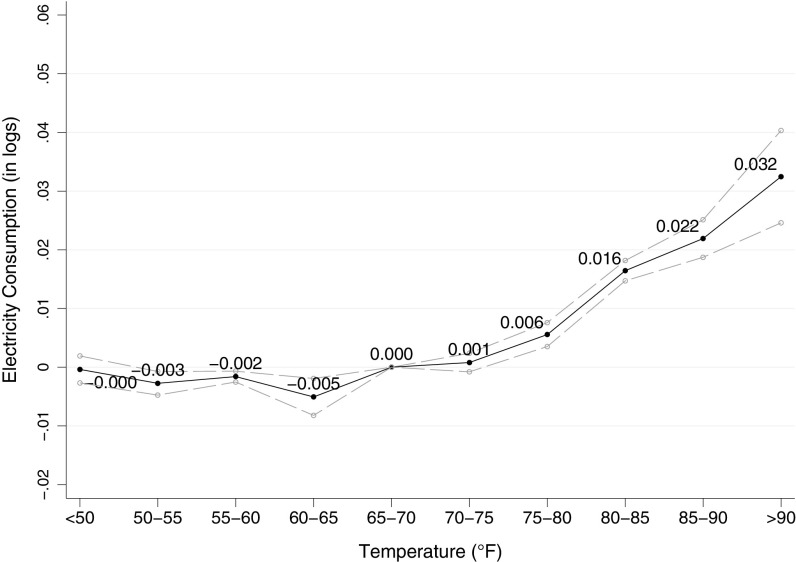
Focusing first on the intensive margin, we use electric billing data to estimate semiparametrically the relationship between temperature and residential electricity consumption. The estimates show large increases in electricity consumption on hot days. For example we find that, relative to a 65–70 °F day, each additional day with a mean temperature exceeding 90 °F increases monthly electricity consumption by 3.2%. Moreover, the results show that the temperature–response function is significantly steeper for households living in states where air conditioning is more prevalent.

For the extensive margin, we use detailed microdata to measure the empirical relationship between climate, income, and air conditioner adoption. We find that what matters most is the interaction between climate and income. In cool areas, air conditioner saturation is near zero for all income levels. In warm areas, however, we find a close relationship between household income and air conditioner adoption, with ownership increasing 2.7 percentage points per $1,000 of annual household income. The relationship is precisely estimated and similar across alternative specifications.

Finally we combine both sets of estimates with predicted end-of-century temperature changes from a set of state-of-the-art climate models. Considering the intensive margin alone, our estimates imply that temperature increases as predicted under the Representative Concentration Pathway (RCP) 8.5 emissions scenario would lead to a 15.4% increase in residential electricity consumption by end of century. This is similar to existing estimates for the United States (6), despite much higher levels of air conditioning saturation in the United States.

The forecast increase in energy use is much larger when we incorporate the extensive margin. Under modest assumptions about income growth, our model implies that the fraction of households with air conditioning will increase from 13% today to more than 70% by end of century. With many more air conditioners in use, our estimates imply an 83% increase in residential electricity consumption by end of century under RCP 8.5.

Our paper differs from most previous studies of the effect of climate on energy consumption. First, most previous work has focused only on the intensive margin (6–8), or only on the extensive margin (9), but our analysis examines both margins. Second, our paper is unusual because most previous studies have used data from the United States. Most of the growth in energy consumption over the next several decades is forecast to come from low- and middle-income countries (10, 11), so evidence from outside the United States is critical.

For this analysis we compiled one of the most comprehensive datasets ever assembled on air conditioning. Whereas most previous analyses of air conditioning have used aggregate data (6, 7, 9, 11–15), our study uses household-level microdata, both on electricity consumption and on air conditioning ownership. These unusually rich data allow us to estimate effects precisely even with highly flexible specifications and to exploit cross-sectional variation across households for identification.

The Intensive Margin

Electricity consumption increases on hot days because people run their air conditioning more. This section examines this intensive margin, describing empirically the relationship between temperature and electricity consumption. We estimate the model using household-level billing data from the universe of more than 25 million Mexican residential customers. This large number of households and rich underlying day-to-day variation in temperature allows us to estimate a highly flexible semiparametric model that controls for time-invariant differences across households and population-wide trends.

Econometric Model.

Our approach can be described with the following regression equation:

$$ln\left(y_{it}\right)={\displaystyle \sum _j{\alpha }_{j}TEM{P}_{itj}+\beta RAI{N}_{it}+{\gamma }_i+{\omega }_t+{\mathit{ϵ}}_{it}}.$$ [1]

The dependent variable $ln\left(y_{it}\right)$ is electricity consumption by household i in billing cycle t, measured in logs. In our data we have 12+ billing cycles for most households. Let $TEM{P}_{itj}$ denote the number of days for household i in billing cycle t in which the mean temperature was in bin j. The parameter ${\alpha }_j$ is a vector of coefficients that measures the change in electricity consumption associated with one additional day in each temperature bin.^†

We include in all regressions a second-order polynomial in total precipitation ($RAI{N}_{it}$) during the billing cycle, household fixed effects ${\gamma }_i$ to control for baseline differences across households, and billing cycle fixed effects ${\omega }_t$ to control for population-wide trends, unmodeled seasonal patterns, and other time effects. The error term ${\mathit{ϵ}}_{it}$ reflects differences in consumption not explained by the different fixed effects, temperature, and precipitation. In all results we cluster our SEs at the municipality level to allow for arbitrary serial correlation and correlation across households within municipalities.

Identifying Variation in Temperature.

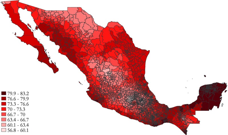
The model is identified using day-to-day variation in temperature. Fig. 1 describes the geographic pattern of mean annual temperature in Mexico. These data come from a database that we constructed of daily weather by municipality using records from hundreds of monitoring stations archived by the US National Climatic Data Center. The figure reveals rich variation in temperature, with average temperature ranging from below $60°\text{F}$ in parts of the central plateau, to above $80°\text{F}$ on the coasts and in the Yucatan peninsula.

Fig. 1.

Mean temperature ($°\text{F}$).

As this figure illustrates, Mexico is an ideal setting for an empirical study of air conditioning because of its varied climate. The country is 2,000+ miles long, with populated areas located from sea level up to 8,000 feet, and with climate zones ranging from hot and humid tropical to arid deserts to high-altitude plateaus.

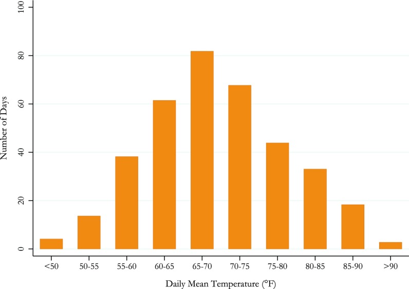
Fig. 2 plots the distribution of mean daily temperature. Each bar represents the average number of days per year experienced in each temperature bin. On average, households experience 80 d per year in which the average temperature is between $65$ and $70°\text{F}$. The distribution is approximately normal, with few days for which the average temperature is below $50°\text{F}$, and few days above $90°\text{F}$. These are average daily measures over an entire day (24 h), so $90°\text{F}$ is an extremely hot day.

Fig. 2.

Daily mean temperature, weighted by population.

Baseline Estimates.

Fig. 3 plots our estimates of the effect of temperature on electricity consumption. We plot estimated coefficients and 95th percentile confidence intervals corresponding to all 10 temperature bins. Between $50$ F and $70°\text{F}$ there is essentially zero effect of temperature on electricity consumption. Electricity consumption increases starting in the $75$–$80°$ bin, with progressively larger impacts in the $80$–$85°$, $85$–$90°$, and $>90°$ bins. The excluded category is $65$–$70°$ so all estimates can be interpreted relative to this baseline.

Fig. 3.

The effect of temperature on residential electricity demand.

The near-zero estimate on $<50°$ days is interesting. Estimated temperature–response functions for the United States are “U”-shaped, with increases in electricity consumption on both hot and cold days (6, 8). With a U shape as average temperatures rise there is increased electricity consumption for cooling but also decreased electricity consumption for heating. Our estimates imply no such offsetting decrease, so the net impact of climate change could be considerably larger. This lack of a response on cold days makes sense given that few Mexican households have electric heating.

We find that each additional day in the $>90°$ bin increases monthly electricity consumption by 3.2%. This is similar in magnitude to existing estimates for the United States despite the wide difference in air conditioning saturation.^‡ In additional results reported in Supporting Information, we find that there is a considerable amount of temperature response even in states with low levels of air conditioning saturation. This likely reflects the use of fans and other substitutes for air conditioning.^§ In addition, we find that the temperature–response function is significantly steeper in states with high levels of air conditioning (p value $<.01$).

The Extensive Margin

In this section we turn to examining the extensive margin using data from the Encuesta Nacional de Ingresos y Gastos de los Hogares (ENIGH), a nationally representative in-home household survey with more than 27,000 respondents in 2010. Using these data we describe empirically the relationship between climate, household income, and the adoption of air conditioning. We find that both climate and income are important in predicting air conditioner adoption, but that the interaction between the two is considerably more important than the individual factors by themselves.

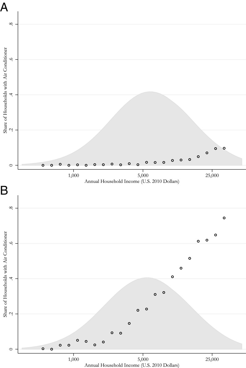
Fig. 4 plots air conditioning saturation as a function of annual household income. We present separate figures for cool and warm municipalities, defined as below and above the mean number of annual CDDs nationally. Household income is measured in US 2010 dollars and the endpoints include all households with annual income less than $500 or greater than $30,000, respectively. In gray is the histogram for annual household income. Plotted in log scale, the distribution is approximately normal, with relatively few households outside these endpoints.

Fig. 4.

Income, climate, and air conditioning. (A) Municipalities with below-average CDDs. (B) Municipalities with above-average CDDs.

In cool municipalities, there is little air conditioning at all income levels. Saturation increases modestly with income, but even among households with more than $30,000 in annual income the saturation of air conditioning never exceeds 10%. In warm municipalities the pattern is very different. Saturation begins low but then increases steadily to near 80%. These are raw shares; these data have not been smoothed, yet air conditioning shares increase almost monotonically.

We show corresponding regression estimates in Table S1. In the standard specification, air conditioning ownership increases by 3 percentage points per $10,000 in annual household income in cool places, while increasing by 27 percentage points per $10,000 in warm places. The relationship is robust and strongly statistically significant across specifications including models that control for region and state fixed effects.

Related work has documented the role of climate and income in US air conditioning adoption between 1960 and 1980 (9), and modeled US demand for air conditioners between 1987 and 2005 using a dynamic structural model (24). Apart from these papers, however, there is surprisingly little work in the economics literature on adoption of air conditioners, particularly on the role of climate (25).

Forecasting End-of-Century Energy Use

Since the 1950s global average temperature has increased $1.3°\text{F}$ and most climate models predict additional increases of $1.8°\text{F}$ or more by the end of the century (26). In this section we combine our estimates with temperature change predictions from a set of state-of-the-art climate models to forecast end-of-century electricity consumption, electricity expenditures, and carbon dioxide emissions.

Temperature Predictions.

To construct the end-of-century temperature predictions, we started with current temperatures and then added predicted temperature changes by month of year from Climate Wizard (www.climatewizard.org/). To capture the rich cross-sectional variation, we used separate temperature distributions for each municipality and predicted temperature changes with a high degree of geographic detail.

We report results for temperature increases corresponding to RCP 4.5 and RCP 8.5, two potential scenarios for greenhouse gas concentration trajectories adopted by the Intergovernmental Panel on Climate Change for its Fifth Assessment Report. With RCP 4.5 emissions peak around 2040 and then stabilize, with carbon dioxide concentration levels around 500 parts per million. RCP 8.5 is essentially “business as usual” with emissions increasing throughout the century and carbon dioxide concentrations reaching 900 parts per million by end of century. For each scenario we use average predicted temperature changes from the 25 climate models that have partnered with Climate Wizard.

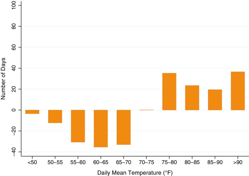
Fig. 5 plots the change in the population-weighted temperature distribution by 2070–2099 in the RCP 8.5 scenario. The four highest temperature bins increase dramatically. On average, households experience almost 40 more days per year in which the average temperature is above $90°\text{F}$. Under the RCP 4.5 scenario the temperature increases are about half as large, but the overall pattern is similar with a significant increase in the four highest temperature bins.

Fig. 5.

Changes in daily mean temperature, RCP 8.5 emissions scenario.

Forecasts: Intensive Margin Only.

The upper half of Table 1 shows the end-of-century impacts implied by our estimates of the temperature–response function. These forecasts come directly from our estimates of the intensive margin (i.e., Fig. 3) and thus should be viewed as holding the current stock of cooling equipment fixed. We calculated the change in electricity consumption by multiplying each element of the temperature–response function by the predicted change in the number of days in each temperature bin, and then taking the sum of these products.

Table 1.

End-of-century predictions

Greenhouse gas concentration trajectory	Households with air conditioning, %	Change in residential electricity consumption (compared with 2010), %	Total change in annual electricity expenditure (US 2010 dollars, millions)	Total change in annual carbon dioxide emissions, millions of tons
	Intensive margin only
RCP 4.5	13	7.5	$357	2.7
RCP 8.5	13	15.4	$733	5.5
	Intensive and extensive margins, with 2% annual income growth
RCP 4.5	71	64.4	$3,065	23.1
RCP 8.5	81	83.1	$3,955	29.8

Under the RCP 4.5 scenario, electricity consumption increases by 7.5%. This reflects more intensive use of air conditioners as well as increased electricity consumption by fans, refrigerators, and other cooling equipment. In 2010, total residential expenditures on electricity in Mexico were $4.8 billion and total associated carbon dioxide emissions were 35.9 million tons (Supporting Information). Consequently, a 7.5% increase implies that electricity expenditures go up by $357 million annually and carbon dioxide emissions increase by 2.7 million tons per year. Impacts are about twice as large under the RCP 8.5 scenario.

The estimated percentage changes are similar to previous estimates from the United States.^¶ One might have expected a smaller increase in Mexico given the lower saturation of air conditioning. However, the shape of the temperature–response function makes a big difference. The U-shaped temperature–response function in the United States implies a large offsetting decrease in consumption from fewer cold days. In contrast, we find little temperature response on cold days, so temperature changes increase electricity consumption unambiguously.

Forecasts: Incorporating the Extensive Margins.

The lower half of Table 1 shows predictions that allow for changes along both the intensive and extensive margins. For these calculations, we assume that household income will increase by 2% annually. This is likely conservative. The US Department of Energy, for example, predicts that Mexican gross domestic product (GDP) will grow at 3.7% annually between 2010 and 2040 (27). With 2% annual growth, household income increases approximately fourfold over the next 70 y.

Under the RCP 4.5 scenario, air conditioning saturation increases to 71% by end of century. For this prediction we use the fully specified adoption model, along with predicted household income and CDDs for end of century. Electricity consumption increases by 64%, with electricity expenditures and carbon dioxide emissions increasing proportionally. Impacts are larger under the RCP 8.5 scenario, with air conditioning saturation at 81%, and an 83% increase in electricity consumption. These are large changes, implying $3+ billion in increased annual electricity expenditures and a 23+ million ton annual increase in carbon dioxide emissions.

Thus, the predicted increases in electricity consumption are much larger after incorporating the extensive margin. This is likely to be true not only in Mexico, but also in middle- and low-income countries around the world. High-income countries already have high levels of air conditioning, so the intensive margin is most important. However, saturation levels are much lower in the rest of the world, so it is this extensive margin that will matter most. Increased saturation of air conditioners has important implications not only for total electricity generation and carbon dioxide emissions, but also for load management. Many parts of the world have, or are gaining, a pronounced seasonal peak in electricity demand corresponding to the hottest months of the year (13), so increased air conditioning could necessitate large capacity investments.

Another striking feature of these predictions is the similarity between RCP 4.5 and RCP 8.5. Global temperatures are much higher under RCP 8.5, and this indeed leads to higher electricity consumption, but income growth by itself explains most of the increase in air conditioning. Even with 2% annual income growth, saturation levels reach near 100% in all warm areas under both scenarios. This is another pattern that we would expect to hold not only in Mexico, but also in the rest of the world. Our estimates show that saturation levels are extremely sensitive to changes in income so even modest income growth, when compounded over several decades, will spur substantial increases in ownership.

To get some sense of the global implications, Table 2 describes the top 12 countries in terms of air conditioning potential, as defined by Sivak (3) as the product of population and CDDs. Excluding the United States, the list is dominated by middle- and low-income countries with warm climates. A total of almost 4 billion people live in these 11 countries, subject to an average of 2,700 annual CDDs. Mexico ranks number 12 but has less than half the CDDs experienced by India, Indonesia, Philippines, and Thailand. Moreover, most of the countries on the list are within the income range where in Mexico we begin to observe a rapid increase in air conditioning adoption.

Table 2.

Air conditioning potential, top 12 countries

Country	Population (in millions)	Annual CDDs	Annual GDP per capita (in thousands)
India	1,252	3,120	1.5
China	1,357	1,046	6.8
Indonesia	250	3,545	3.5
Nigeria	174	3,111	3.0
Pakistan	182	2,810	1.3
Bangladesh	157	2,820	1.0
Brazil	200	2,015	11.2
Philippines	98	3,508	2.8
United States	316	882	53.0
Vietnam	90	3,016	1.9
Thailand	67	3,567	5.8
Mexico	122	1,560	10.3

Conclusion

Our results point to the enormous potential global impacts from air conditioning. We find large increases in electricity consumption on hot days, with essentially no offsetting impact from reduced heating on cold days. Our results also reveal the remarkable speed with which air conditioning adoption increases with income. Under modest assumptions about income growth, our model predicts near-universal saturation of air conditioning in all warm areas within just a few decades. Temperature increases contribute to this increased adoption, but income growth by itself explains the lion’s share.

Whether or not these forecasts will prove accurate depends on the pace of technological change. There have been dramatic improvements in energy efficiency over the last several decades, in part due to induced innovation (28), and as the market for air conditioning grows this will increase incentives for firms to innovate (29). Continued advances in energy efficiency or the development of new cooling technologies could reduce the energy consumption impacts considerably. Similarly, growth in low-carbon electricity generation could substantially mitigate the carbon dioxide impacts.

The future pattern of air conditioning adoption and use will also reflect what happens to prices. Equipment prices are likely to continue to decrease, which would further accelerate adoption. What will happen to electricity prices is less clear. A substantial increase in electricity prices, for example, resulting from carbon legislation, would slow both adoption and use. Moreover, the increased use of real-time electricity prices would lower peak consumption, reducing the need for additional investments in capacity.

Finally, there is a whole set of broader adaptations that over a long time period could substantially reduce the need for air conditioning. Previous studies have found that people move away from regions affected by extreme temperature and other climatic variations (30, 31), so we would expect migration both within and across countries in response to climate change. Demand for cooling also depends to a large degree on how we build our homes and businesses. These choices are not exogenous; they respond to changes in climate as well as the availability and cost of cooling technologies.

References

- 1.US Department of Energy 2014. Residential Energy Consumption Survey. Available at www.eia.gov/consumption/residential/
- 2.Euromonitor International . Air Treatment Products in China. Euromonitor International; Shanghai, China: 2014. [Google Scholar]
- 3.Sivak M. Will air conditioning put a chill on the global energy supply? Am Sci. 2013;101(5):330–333. [Google Scholar]
- 4.Hausman J. Individual discount rates and the purchase and utilization of energy-using durables. Bell J Econ. 1979;10(1):33–54. [Google Scholar]
- 5.Dubin J, McFadden D. An econometric analysis of residential electric appliance holdings and consumption. Econometrica. 1984;52(2):345–362. [Google Scholar]
- 6.Deschênes O, Greenstone M. Climate change, mortality, and adaptation: Evidence from annual fluctuations in weather in the U.S. Am Econ J Appl Econ. 2011;3(4):152–185. [Google Scholar]
- 7.Franco G, Sanstad AH. Climate change and electricity demand in California. Clim Change. 2008;87(1):139–151. [Google Scholar]
- 8.Auffhammer M, Aroonruengsawat A. Simulating the impacts of climate change, prices and population on California’s residential electricity consumption. Clim Change. 2011;109(1):191–210. [Google Scholar]
- 9.Biddle J. Explaining the spread of residential air conditioning, 1955-1980. Explor Econ Hist. 2008;45(4):402–423. [Google Scholar]
- 10.Wolfram C, Shelef O, Gertler P. How will energy demand develop in the developing world? J Econ Perspect. 2012;26(1):119–138. [Google Scholar]
- 11.Auffhammer M, Wolfram C. Powering up China: Income distributions and residential electricity consumption. Am Econ Rev. 2014;104(5):575–580. [Google Scholar]
- 12.Sailor D, Pavlova A. Air conditioning market saturation and long-term response of residential cooling energy demand to climate change. Energy. 2003;28(9):941–951. [Google Scholar]
- 13.Isaac M, Van Vuuren D. Modeling global residential sector energy demand for heating and air conditioning in the context of climate change. Energy Policy. 2009;37(2):507–521. [Google Scholar]
- 14.McNeil M, Letschert V. Modeling diffusion of electrical appliances in the residential sector. Energy Build. 2010;42(6):783–790. [Google Scholar]
- 15.Auffhammer M. Cooling China: The weather dependence of air conditioner adoption. Frontiers Econ China. 2014;9(1):70–84. [Google Scholar]
- 16.Deschênes O, Greenstone M. The economic impacts of climate change: evidence from agricultural output and random fluctuations in weather. Am Econ Rev. 2007;97(1):354–385. [Google Scholar]
- 17.Schlenker W, Roberts MJ. Nonlinear temperature effects indicate severe damages to U.S. crop yields under climate change. Proc Natl Acad Sci USA. 2009;106(37):15594–15598. doi: 10.1073/pnas.0906865106. [DOI] [PMC free article] [PubMed] [Google Scholar]
- 18.Deschênes O, Greenstone M, Guryan J. Climate change and birth weight. Am Econ Rev. 2009;99(2):211–217. doi: 10.1257/aer.99.2.211. [DOI] [PubMed] [Google Scholar]
- 19.Dell M, Jones B, Olken B. Temperature shocks and economic growth: Evidence from the last half century. Am Econ J Macro. 2012;4(3):66–95. [Google Scholar]
- 20.Barreca A, Clay K, Deschênes O, Greenstone M, Shapiro JD. 2013. Adapting to climate change: The remarkable decline in the U.S. temperature-mortality relationship over the 20th century. J Polit Econ, in press.
- 21.Deryugina T, Hsiang SM. 2014. Does the environment still matter? Daily temperature and income in the United States. NBER Working Paper 20750 (National Bureau of Economic Research, Cambridge, MA)
- 22.Meier A. Refrigerator energy use in the laboratory and in the field. Energy Build. 1995;22(3):233–243. [Google Scholar]
- 23.Zivin JG, Neidell M. Temperature and the allocation of time: Implications for climate change. J Labor Econ. 2014;32(1):1–26. [Google Scholar]
- 24.Rapson D. Durable goods and long-run electricity demand: Evidence from air conditioner purchase behavior. J Environ Econ Manage. 2014;68(1):141–160. [Google Scholar]
- 25.Auffhammer M, Mansur E. Measuring climatic impacts on energy consumption: A review of the empirical literature. Energy Econ. 2014;46:522–530. [Google Scholar]
- 26.Intergovernmental Panel on Climate Change 2013. Climate Change 2013: The Physical Science Basis. Contribution of Working Group I to the Fifth Assessment Report of the Intergovernmental Panel on Climate Change, eds Stocker TF et al. (Cambridge Univ Press, Cambridge, UK)
- 27.US Department of Energy . International Energy Outlook. US Department of Energy; Washington, DC: 2013. [Google Scholar]
- 28.Newell RG, Jaffe AB, Stavins RN. The induced innovation hypothesis and energy-saving technological change. Q J Econ. 1999;114(3):941–975. [Google Scholar]
- 29.Acemoglu D, Linn J. Market size in innovation: Theory and evidence from the pharmaceutical industry. Q J Econ. 2004;119(3):1049–1090. [Google Scholar]
- 30.Munshi K. Networks in the modern economy: Mexican migrants in the U.S. labor market. Q J Econ. 2003;118(2):549–599. [Google Scholar]
- 31.Bohra-Mishra P, Oppenheimer M, Hsiang SM. Nonlinear permanent migration response to climatic variations but minimal response to disasters. Proc Natl Acad Sci USA. 2014;111(27):9780–9785. doi: 10.1073/pnas.1317166111. [DOI] [PMC free article] [PubMed] [Google Scholar]
Associated Data
This section collects any data citations, data availability statements, or supplementary materials included in this article.