Longitudinal graph-based segmentation of macular OCT using fundus alignment

Abstract

Segmentation of retinal layers in optical coherence tomography (OCT) has become an important diagnostic tool for a variety of ocular and neurological diseases. Currently all OCT segmentation algorithms analyze data independently, ignoring previous scans, which can lead to spurious measurements due to algorithm variability and failure to identify subtle changes in retinal layers. In this paper, we present a graph-based segmentation framework to provide consistent longitudinal segmentation results. Regularization over time is accomplished by adding weighted edges between corresponding voxels at each visit. We align the scans to a common subject space before connecting the graphs by registering the data using both the retinal vasculature and retinal thickness generated from a low resolution segmentation. This initial segmentation also allows the higher dimensional temporal problem to be solved more efficiently by reducing the graph size. Validation is performed on longitudinal data from 24 subjects, where we explore the variability between our longitudinal graph method and a cross-sectional graph approach. Our results demonstrate that the longitudinal component improves segmentation consistency, particularly in areas where the boundaries are difficult to visualize due to poor scan quality.

1. INTRODUCTION

Optical coherence tomography (OCT) has become an increasingly popular modality for examining the retina due to its rapid acquisition time and micrometer-scale resolution. The retina is made up of 11 layers, eight of which are readily distinguishable on currently available imaging technologies. From vitreous to choroid these identifiable layers are: retinal nerve fiber (RNFL), ganglion cell & inner plexiform (GCIP), inner nuclear (INL), outer plexiform (OPL), outer nuclear (ONL), inner segment (IS), outer segment (OS), and retinal pigment epithelium (RPE). OCT images of the macula allow the thickness of these layers to be accurately measured. Clinically, changes in some of these thicknesses reflect retinal pathology associated with various diseases. For example, in multiple sclerosis (MS) the thickness of the RNFL is believed to decrease by approximately 1.0 μm per year,¹ with another study showing changes of only 0.2-0.4 μm per year when averaged over the macula.² Since MS and other diseases are progressive with time, it is important to track these changes accurately.

Many automated algorithms have been developed for segmentation of retinal layers in OCT data,^3–9 but none incorporate longitudinal consistency. The accuracy of these algorithms is generally >4 μm, making them insensitive to detecting small temporal changes of the type seen in MS. Other factors including blood vessel shadowing, scan misalignment, low SNR, the appearance of Henle's fiber layer,¹⁰ and ambiguities in layer boundary positions in the deeper retina¹¹ contribute to errors when comparing two scans acquired at different times.

Graph-based segmentation methods of the type initially presented by Li et al.¹² and later demonstrated in OCT^3,5,6,8,13 are extended in this work to handle longitudinal data. We do this by connecting the separate 3-D graphs constructed at each visit and carrying out a simultaneous 4-D segmentation. This idea was previously used for the segmentation of lung data.¹⁴ The temporally-connected graph edges serve to regularize the result over time. However, this simple connection of the graphs is not trivial because voxel correspondences over time are unknown. Before construction of this temporal graph, we propose to first align the data to find appropriate graph correspondences. We do not use traditional 3-D image registration methods due to the highly anisotropic nature of OCT data, with through-plane resolution up to 25 times worse than the in-plane direction. Instead, we take advantage of the consistent geometry of the data whereby we are able to find an alignment in the axial direction separately from the transverse and through-plane directions. We first outline the alignment of the data, followed by describing the framework used for the final graph-based segmentation.

2. METHODS

For this study, we used macular OCT data (20° × 20°) acquired from a Heidelberg Spectralis scanner (Heidelberg Engineering, Heidelberg, Germany), which covered approximately a 6 6 mm area centered at the fovea. The volumetric dimensions of each scan are 1024 × 49 × 496 voxels in the x, y, and z directions, which represent the lateral, through-plane, and axial directions, respectively. We denote an in-plane image as a B-scan (in the xz-plane), and an axial scan line as an A-scan. The voxel spacing is approximately 5.8 × 123 × 3.9 μm, thus the data is highly anisotropic.

For our final segmentation method, we represent each individual volume of the OCT data using a graph whereby each voxel corresponds to a vertex. To carry out our longitudinal segmentation, we add edges connecting corresponding vertices in the graphs at adjacent visits (i.e. the second visit is connected to the first and third visits only). To make these connections, we require that the data is first aligned. Before describing the full longitudinal graph segmentation algorithm in Sec. 2.4, we first describe the multi-step registration of the longitudinal data, which begins with an initial boundary segmentation.

2.1 Initial boundary segmentation

As the first step in aligning the data, we independently perform a low resolution segmentation (LRS) of each longitudinal scan using the graph-based algorithm described in Sec. 2.4 cross-sectionally. We use the LRS to generate reference surfaces, useful both for registering the data to a common boundary and for increasing the efficiency of the final graph segmentation by reducing the graph search space. To get the LRS, we downsample the data by a factor of 20 in the x direction, thus making the LRS quick to compute while providing sufficient accuracy for later use. From the LRS, for each time point t, we form 9 boundary estimates {r_k(x,y,t)ǀk ∈ {,...,9}} where r_k(x,y,t) is the height of the boundary each in A-scan, and k specifies an ordering from the inner retina.

2.2 Axial alignment

Given the LRS at each visit, we flatten the data to the estimated IS-OS boundary by translating each A-scan in the axial direction until this boundary lies flat in each image. Thus, each scan is transformed as I_f(x,y,z,t) = I(x, y,z,t) = I(x,y,z – r₇(x,y) + α,t) where α is a constant placing the flat surface at an arbitrary height. We use the IS-OS boundary as it is accurately estimated, even in the LRS, due to its sharp intensity gradient. After flattening, we assume that each longitudinal scan is aligned in the axial direction, i.e. z = 1 corresponds to the same position for all t. We show an example of this axial alignment step, in addition to the LRS, in Fig. 1.

Figure 1.

B-scan images from the same subject at three different visits after alignment to the IS-OS boundary. Boundaries estimated from the LRS are overlaid.

2.3 Fundus alignment by vessel registration

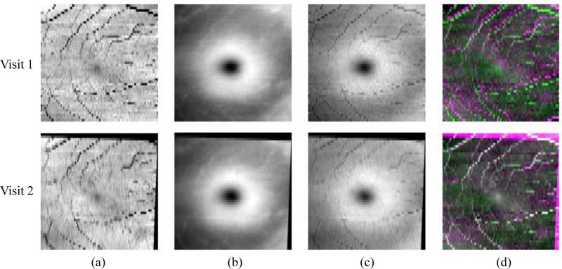
Next, we align the data in the xy-plane using fundus projection images (FPIs), constructed as a combination of total retina thickness maps, T , and vessel shadow projections, S, both generated using the LRS. The thickness maps are computed as the difference between the top and bottom boundary,

$$T(x,y,t)=r_1(x,y,t)-r_9(x,y,t),$$ (1)

while the vessel maps are computed from the sum of intensities above the bottom boundary

$$S(x,y,t)=\sum _{z=r_9(x,y,t)}^{r_9(x,y,t)+15}I(x,y,z,t).$$ (2)

After normalizing the intensity range of both S and T to [0,1], we get the final FPI as F(x,y,t) = S(x,y,t) + γT(x,y,t). The FPIs enable us to generate correspondences based on vessel locations and guide the registration using the foveal shape information, particularly at the fovea where there are no vessels.

The FPIs for each visit are registered pairwise to the baseline FPI using an a ne transformation and the mutual information similarity measure. Figure 2 shows S, T , and F for two visits of the same subject, and the resulting alignment of the F's after the a ne registration. Note that we empirically use a value of γ = 2 when generating the FPIs, which exhibits good registration performance.

Figure 2.

Fundus registration of 2 visits. Columns (a), (b), and (c) show the vessel shadow projection images S, the retina thickness images T , and the combined FPIs, respectively. In (d), we show color overlay images (top) before and (bottom) after registration. White indicates the improved alignment of the vessels.

2.4 Graph-based segmentation

At this point, we assume the longitudinal data is registered in all three dimensions. Since the scans are only aligned based on a single surface in the axial direction, we assume that any differences in the remaining surfaces are either from noise, or physiological changes perhaps due to disease. By regularizing the difference between the segmentation at separate visits, we hope to smooth out the noise while maintaining any true changes that occur. We segment the final boundaries using a graph-based method that we previously developed and validated.⁸ This algorithm is briefly described next, with the longiduinal extension of the algorithm described in Sec. 2.4.1.

We wish to find nine boundary surfaces within the retina constrained to have a fixed ordering. To do this, we need to find exactly nine boundary points along each A-scan of the data. Given an N_x × N_y × N_z volume and N_s surfaces to find, we search for the set of boundary surfaces {s_k(x,y)|k ∈ {1,...,9}} that minimize

$$\sum _{k=0}^{N_s-1}\sum _{y=0}^{N_y-1}\sum _{x=0}^{N_x-1}{c}_k(x,y,s_k(x,y))\mathrm{s}.\mathrm{t}.s_k(x,y)\ge s_{k^{\prime }}(x,y)\forall k>k^{\prime }$$ (3)

where c_k(x,y,s_k(x,y)) is the cost of placing boundary k at voxel (x,y,s_k(x,y)).

Li et al.¹² described a graph-based algorithm for optimally finding the set of surfaces that minimizes Eq. 3 by careful construction of a graph on the data, which is then solved using a minimum s-t cut.¹⁵ Solving the graph in this manner can produce noisy results since smoothness is not enforced. Thus, hard constraints are introduced which control the minimum and maximum thickness of each layer, and the amount of change between adjacent A-scans.^6,12

For each of the longitudinal scans, we construct a separate graph on the image data following the methods outlined in Refs. 6 and 12. Solving the segmentation problem on each of these graphs separately gives us the traditional cross-sectional graph (CSG) segmentation. Connecting the graphs from adjacent visits will allow us to do a simultaneous longitudinal graph (LG) segmentation. We denote G(t) = (V (t), E(t)) as the graph corresponding to the volume at time point t with each vertex V (x,t) corresponding to a voxel in the data at location x. These vertices are also associated with a boundary cost c_k(x). We use c_k(x) = 1 p(kǀx) where p(kǀx) is the probability that the pixel belongs to boundary k. The boundary probabilities are computed using a random forest classifier,¹⁶ trained using location information and different spatial filters computed at each voxel, details of which are described in our previous work.⁸ The same boundary probability maps are used for the CSG, and LG segmentations, and with downsampling for the LRS.

2.4.1 Longitudinal extension

To extend the graph segmentation algorithm to longitudinal data, we add additional edges between the graphs at adjacent visits. For the case that the data at each visit is perfectly aligned, we can simply add a non-zero weighted bidirectional edge between corresponding voxels at consecutive time points. These edges act to provide a regularization force which penalizes differences in the segmentation result over time. A final segmentation that is identical for each visit would not incur any smoothness penalty since it would not cut any of the added edges.

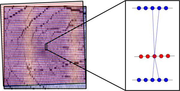
Because of the large distance between B-scan images, we choose not to interpolate the data directly. Thus, we do not have direct correspondences between voxels after the FPI alignment described in Sec. 2.3, which places voxels from the different scans at interpolated positions relative to each other. Connecting the vertices of one volume with the nearest vertex in the next volume is also not satisfactory due to the spacing. Instead, given that the voxel x at t₁ is registered to a (non-integer valued) point x′ at t₂ (from the FPI registration), we connect V(x,t₁) to the four nearest vertices at t₂ found from floor(x′), ceil(x′) and similar for y′ (see Fig. 3). The weight of these edges is set to a value inversely proportional to the distance between the vertices such that the four weights add up to w, which we empirically set w = 0.1. As we maintain the physical location of vertices in the graph, the segmentation is carried out in the native space of each volume instead of on an interpolated grid. Using the described graph with added temporal edges between scans at visits t_i and t_i+1 ∀i ∈ {,...,N_t –1}, we are able to simultaneously solve for the segmentation at all visits of the patient using a single minimum s-t cut.¹⁵

Figure 3.

On the left are the outlines of two fundus images after alignment, with B-scan locations represented by horizontal lines. After registration, the vertices no longer have direct correspondences for connecting the graphs. Therefore, we connect vertices at one visit (red) to the four nearest vertices in the next visit (blue). The weighting of each edge is inversely proportional to the distance, encouraging the final segmentation to look more similar to closer vertices.

As a final note, we substantially reduce the memory and time requirements of the 4-D LG segmentation problem by masking out pixels that are further than 3 pixels from the LRS boundaries. Masking out these pixels both reduces the search space for the algorithm and substantially reduces the size of the longitudinal graph. We also use the same mask for all visits by taking the union of each; this reduces the possibility that a segmentation error in the LRS will affect the final result.

3. EXPERIMENTS AND RESULTS

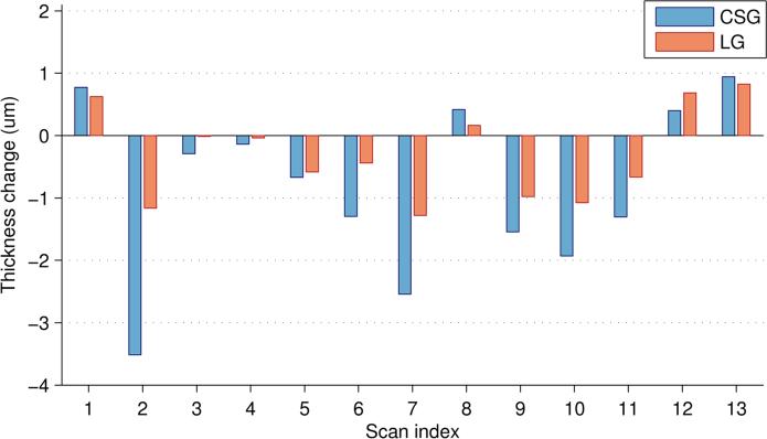
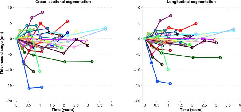
We explored the performance of our LG segmentation on two cohorts. The first included scans of 13 eyes from 7 healthy control (HC) subjects, with all scans repeated approximately one year later. The second data pool contained 34 eyes of 17 patients with MS, each scanned between 3 and 5 times at intervals of 3 to 12 months. We looked at the total retinal thickness as measured from the top of the RNFL to the bottom of the RPE to explore the overall effect of the algorithm. The thickness values were averaged within a 5 × 5 mm square centered at the fovea, where the center of the fovea was defined as the position with the smallest total thickness near the center of the volume. Results of running both the CSG and LG segmentation algorithms on both cohorts are shown in Fig. 4 and Fig. 5, where we see the change in total retina thickness relative to the baseline scan.

Figure 4.

Plot of the change in total retina thickness as compared to the thickness at the baseline visit for 13 HC scans using both the CSG and LG segmentation methods. Repeat scans were acquired approximately 12 months after the baseline.

Figure 5.

Plot of the change in total retina thickness as compared to the thickness at the baseline visit for 34 MS scans. Results for the CSG and LG segmentation methods are shown, with each color representing a single subject.

In the control population (see Fig. 4), the longitudinal regularization reduces the standard deviation of the change in thickness from 1.35 to 0.73 or by 46%. Since this is a control population, we do not expect the measurements to change much over 1 year. We can also use these results as a reference for the amount of variability we expect to see in the CS method. It is also interesting to note that the variability of the CS method is slightly less than the overall variability of the algorithm as previously reported (1.8 μm).⁸ This decrease is expected since we are comparing automated results from similar data as opposed to comparison with manual delineations.

For the MS results in Fig. 5, we see a general smoothing of the results using the LG method as compared to the CSG. Note that the changes are not trending towards zero as we saw with the control data, suggesting that true changes are not being removed and that we are not over regularizing. One method to measure the increased consistency of the LG segmentation is to look at the residual error of a linear fit to the data. In this case, the root mean square fitting error is reduced from an average of 1.83 μm to 1.13 μm (p < 1e-10). Our results also agree with the literature that the overall changes in retinal thickness due to MS are small.^1,2 Some of the larger changes that we see may be due to the onset of optic neuritis or edema,¹⁷ which are known to decrease or increase the thickness of the retina, respectively.

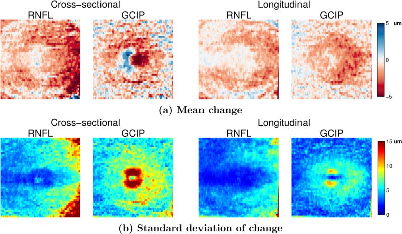
In the previous experiment, we looked at the average thickness over the entire macular area. Next, we explored how different retinal layers change in a localized manner. Fig. 6 shows the average change in the thickness of the RNFL and GCIP layers over one year (relative to the baseline scan) in the MS cohort for both the CS and LG methods. We only show these layers since they are known to be the most affected by MS² and have the most atrophy. We see that the magnitude of the changes in the LG method are smaller than those using the CSG, but the standard deviation is also much smaller. This result means that we have more confidence in localizing the changes using the longitudinal method. Also note that the GCIP shows an area of increased thickness near the fovea using the CSG method which is removed using the LG method; a result which is more consistent with what is known about changes due to MS. This result also informs us that global measures of thickness are less sensitive to finding temporal changes since these changes tend to be localized to specific areas. Averaging the thickness change over the entire macula includes many regions which may not be changing.

Figure 6.

Comparison of the mean and standard deviation of the change in the RNFL and GCIP layer thicknesses using the CSG and LG methods on the MS cohort of scans that have one year of data (24 scans).

Finally, in Fig. 7 we show a comparison of running the CSG and LG algorithms. We see the negative effect that the disappearance of Henle's fiber layer has on the segmentation of the OPL and ONL. The LG regularization maintains consistency over time, even when the boundaries are not clearly visible. Note that this boundary appears more clearly in the adjacent scans in time.

Figure 7.

Improvement in the ONL for the case of the appearance and disappearance of Henle’s fiber layer, with CSG on the left and LG on the right. Information from multiple visits enforces consistency over time.

4. CONCLUSIONS

We have developed a graph-based technique for the segmentation of longitudinal OCT data of the retina. We register the data in two steps, first axially then in the fundus plane, and use the correspondences to connect the graphs. Longitudinal segmentation relies on accurate alignment, so if either of our alignment steps fails, the segmentation will be incorrect. However, our alignment method was quite robust even for low quality data. Our method currently only allows for small changes over time, exploration of this drawback and the influence of w will be explored in future work.

REFERENCES

- 1.Talman LS, Bisker ER, Sackel DJ, Long DA, Galetta KM, Ratchford JN, Lile DJ, Farrell SK, Loguidice MJ, Remington G, Conger A, Frohman TC, Jacobs DA, Markowitz CE, Cutter GR, Ying G-S, Dai Y, Maguire MG, Galetta SL, Frohman EM, Calabresi PA, Balcer LJ. Longitudinal study of vision and retinal nerve fiber layer thickness in multiple sclerosis. Annals of Neurology. 2010;67(6):749–760. doi: 10.1002/ana.22005. [DOI] [PMC free article] [PubMed] [Google Scholar]
- 2.Ratchford JN, Saidha S, Sotirchos ES, Oh JA, Seigo MA, Eckstein C, Durbin MK, Oakley JD, Meyer SA, Conger A, Frohman TC, Newsome SD, Balcer LJ, Frohman EM, Calabresi PA. Active MS is associated with accelerated retinal ganglion cell/inner plexiform layer thinning. Neurology. 2013;80(1):47–54. doi: 10.1212/WNL.0b013e31827b1a1c. [DOI] [PMC free article] [PubMed] [Google Scholar]
- 3.Antony BJ, Abràmo MD, Harper MM, Jeong W, Sohn EH, Kwon YH, Kardon R, Garvin MK. A combined machine-learning and graph-based framework for the segmentation of retinal surfaces in SD-OCT volumes. Biomed. Opt. Express. 2013;4(12):2712–2728. doi: 10.1364/BOE.4.002712. [DOI] [PMC free article] [PubMed] [Google Scholar]
- 4.Chiu SJ, Li XT, Nicholas P, Toth CA, Izatt JA, Farsiu S. Automatic segmentation of seven retinal layers in SDOCT images congruent with expert manual segmentation. Opt. Express. 2010;18(18):19413–19428. doi: 10.1364/OE.18.019413. [DOI] [PMC free article] [PubMed] [Google Scholar]
- 5.Dufour PA, Ceklic L, Abdillahi H, Schroder S, De Zanet S, Wolf-Schnurrbusch U, Kowal J. Graph-based multi-surface segmentation of OCT data using trained hard and soft constraints. IEEE Trans. Med. Imag. 2013;32(3):531–543. doi: 10.1109/TMI.2012.2225152. [DOI] [PubMed] [Google Scholar]
- 6.Garvin M, Abramo M, Wu X, Russell S, Burns T, Sonka M. Automated 3-D intraretinal layer segmentation of macular spectral-domain optical coherence tomography images. IEEE Trans. Med. Imag. 2009;28(9):1436–1447. doi: 10.1109/TMI.2009.2016958. [DOI] [PMC free article] [PubMed] [Google Scholar]
- 7.Ghorbel I, Rossant F, Bloch I, Tick S, Paques M. Automated segmentation of macular layers in OCT images and quantitative evaluation of performances. Pattern Recognition. 2011;44(8):1590–1603. [Google Scholar]
- 8.Lang A, Carass A, Hauser M, Sotirchos ES, Calabresi PA, Ying HS, Prince JL. Retinal layer segmentation of macular OCT images using boundary classification. Biomed. Opt. Express. 2013;4(7):1133–1152. doi: 10.1364/BOE.4.001133. [DOI] [PMC free article] [PubMed] [Google Scholar]
- 9.Vermeer KA, van der Schoot J, Lemij HG, de Boer JF. Automated segmentation by pixel classification of retinal layers in ophthalmic OCT images. Biomed. Opt. Express. 2011;2(6):1743–1756. doi: 10.1364/BOE.2.001743. [DOI] [PMC free article] [PubMed] [Google Scholar]
- 10.Lujan BJ, Roorda A, Knighton RW, Carroll J. Revealing Henle’s fiber layer using spectral domain optical coherence tomography. Invest. Ophthalmol. Vis. Sci. 2011;52(3):1486–1492. doi: 10.1167/iovs.10-5946. [DOI] [PMC free article] [PubMed] [Google Scholar]
- 11.Spaide RF, Curcio CA. Anatomical correlates to the bands seen in the outer retina by optical coherence tomography: Literature review and model. Retina. 2011;31(8):1609–1619. doi: 10.1097/IAE.0b013e3182247535. [DOI] [PMC free article] [PubMed] [Google Scholar]
- 12.Li K, Wu X, Chen D, Sonka M. Optimal surface segmentation in volumetric images - a graph-theoretic approach. IEEE Trans. Pattern Anal. Mach. Intell. 2006;28(1):119–134. doi: 10.1109/TPAMI.2006.19. [DOI] [PMC free article] [PubMed] [Google Scholar]
- 13.Song Q, Bai J, Garvin M, Sonka M, Buatti J, Wu X. Optimal multiple surface segmentation with shape and context priors. IEEE Trans. Med. Imag. 2013;32(2):376–386. doi: 10.1109/TMI.2012.2227120. [DOI] [PMC free article] [PubMed] [Google Scholar]
- 14.Petersen J, Modat M, Cardoso M, Dirksen A, Ourselin S, de Bruijne M. Lecture Notes in Computer Science. Vol. 8150. Springer; 2013. Quantitative airway analysis in longitudinal studies using groupwise registration and 4d optimal surfaces; pp. 287–294. Medical Image Computing and Computer-Assisted Intervention — MICCAI 2013. [DOI] [PubMed] [Google Scholar]
- 15.Boykov Y, Kolmogorov V. An experimental comparison of min-cut/max-flow algorithms for energy minimization in vision. IEEE Trans. Pattern Anal. Mach. Intell. 2004;26(9):1124–1137. doi: 10.1109/TPAMI.2004.60. [DOI] [PubMed] [Google Scholar]
- 16.Breiman L. Random forests. Machine Learning. 2001;45(1):5–32. [Google Scholar]
- 17.Saidha S, Sotirchos ES, Ibrahim MA, Crainiceanu CM, Gelfand JM, Sepah YJ, Ratchford JN, Oh J, Seigo MA, Newsome SD, Balcer LJ, Frohman EM, Green AJ, Nguyen QD, Calabresi PA. Microcystic macular oedema, thickness of the inner nuclear layer of the retina, and disease characteristics in multiple sclerosis: a retrospective study. The Lancet Neurology. 2012;11(11):963–972. doi: 10.1016/S1474-4422(12)70213-2. [DOI] [PMC free article] [PubMed] [Google Scholar]