

Abstract
An increasing number of organisms can be fully 13C-labeled, which has the advantage that their metabolomes can be studied by high-resolution 2D NMR 13C–13C constant-time (CT) TOCSY experiments. Individual metabolites can be identified via database searching or, in the case of novel compounds, through the reconstruction of their backbone-carbon topology. Determination of quantitative metabolite concentrations is another key task. Because significant peak overlaps in 1D NMR spectra prevents straightforward quantification through 1D peak integrals, we demonstrate here the direct use of 13C–13C CT-TOCSY spectra for metabolite quantification. This is accomplished through the quantum-mechanical treatment of the TOCSY magnetization transfer at short and long mixing times or by the use of analytical approximations, which are solely based on the knowledge of the carbon-backbone topologies. The methods are demonstrated for carbohydrate and amino-acid mixtures.
Keywords: Metabolomics, quantitative NMR, 13C-labeled organisms, constant-time TOCSY
Introduction
Due to its versatility and quantitative nature, nuclear magnetic resonance (NMR) spectroscopy is one of the most commonly used tools in analytical chemistry.1,2 1D 1H NMR experiments are widely applied for the extraction of quantitative concentrations of individual chemical species in solution provided that the spectra are well-resolved. A major advantage of 1D 1H spectra is that the integral of a given peak is directly proportional to the concentration of the compound it belongs to.3 1D 13C{1H} NMR spectroscopy at natural 13C abundance can also be used for quantification by targeted profiling using database information.4
In the presence of strong peak overlaps, which are typical for complex mixtures such as ones encountered in metabolomics, alternative methods are required. While the resolution issue can often be overcome by 2D NMR spectroscopy, the quantification of 2D spectra is hindered by the variability of cross-peak intensities due to uneven magnetization transfer during the preparation, evolution, or mixing periods because of differences in scalar J-couplings and spin relaxation.5 This prevents the direct use of cross-peak integrals as quantitative measures of sample concentrations requiring more elaborate approaches that translate cross-peak integrals into concentrations.
2D NMR quantification methods can be divided into two main groups based on their strategies to deal with the variability of cross-peak intensities mentioned above. The first category uses an internal standard for each type of molecule. This approach has been demonstrated for the heteronuclear 2D 13C–1H HSQC6,7 and the homonuclear 2D 1H–1H TOCSY8 and 2D 1H-INADEQUATE experiments.9 It is rather labor-intensive as it requires the preparation and measurement of a large number of standards. Furthermore, molecules identified in a sample cannot be quantified if their standard is unknown, which includes newly discovered molecules. The second approach aims at minimizing the variability in cross-peak intensities by modification of 13C–1H HSQC experiments,10–13 in some cases by extrapolation of a series of experiments.12 It has the advantage that it does not require an internal standard for each molecule.
The 2D NMR quantification techniques mentioned so far are for metabolite samples at natural 13C abundance. Uniform 13C-enrichment of organisms, which is possible for an increasing number of organisms, such as bacteria, yeast, C. elegans, and plants, leads to fully 13C-labeled metabolites. It has recently been demonstrated that homonuclear 13C-NMR of complex mixtures of such metabolites offers unique information about their identity and composition. Based on 2D 13C–13C constant-time (CT) TOCSY NMR spectra, the determination of 112 carbon-backbone topologies of metabolites in a single sample of uniformly 13C-labeled E. coli could be achieved.14 In order to optimally utilize the chemical and biological information of such samples, the quantification of individual mixture components is important. Here, we present general strategies for the quantification of uniformly 13C labeled metabolites, which do not require an internal standard for each metabolite. The proposed strategies are either based on the exact quantum-mechanical simulation of 2D CT-TOCSY NMR spectra or on analytical approximations of the exact simulations.15–17
Methods
Computational approaches for quantification of 2D 13C–13C CT-TOCSY
Quantum-mechanical description of cross-peak volumes
The NMR pulse sequence of the 2D 13C–13C CT-TOCSY experiment18 is shown in Figure S-1. Constant-time evolution during t1 removes the dominant homonuclear 1J(13C,13C) couplings along the indirect dimension ω1. The 2D time-domain signal is given by
| (1) |
where A is a spectrometer-dependent prefactor, ci is the concentration of the metabolite that contains 13C spin Si, T is the duration of the constant-time interval, 1Jik denotes the 1J(13C, 13C) coupling of spin Si to its directly bonded neighbor 13C spin Sk, T2i is the T2 relaxation time of spin Si and Ωi is its Larmor frequency. N denotes the number of spins Si and 22−N is a normalization factor. Siz denotes the spin angular momentum product operator along z of spin i, “Tr” denotes the matrix trace and Hiso the isotropic mixing Hamiltonian during TOCSY mixing:19
| (2) |
2D Fourier transformation of s(t1, t2) of Eq. (1) leads to the 2D NMR spectrum S(ω1,ω2). Because of the linearity of the Fourier transform, the integral (volume) of the cross-peak between spins Si and Sj corresponds to
| (3) |
It follows that the concentration ci of the metabolite that contains the two spins can be estimated according to ci = Vij/Afij where the transfer function
| (4) |
and the universal prefactor A can be empirically determined as described below. The transfer function of Eq. (4) can be computed because all parameters are either known or can be estimated with good accuracy. Specifically, because in 13C spin systems the 1J(13C, 13C) couplings, which range between 30 – 55 Hz, dominate the geminal 2J(13C, 13C) and vicinal 3J(13C, 13C) couplings, knowledge of the backbone topology of a metabolite permits the straightforward determination of Hiso (Eq. (2)). Furthermore, since for metabolites the transverse relaxation times T2 by far exceed the constant-time period T, is close to 1 for all metabolites so that it can be incorporated in prefactor A. T1 and T2 relaxation effects during the TOCSY mixing time τm can be treated in the same way. The constant-time period T is chosen so that T = 1/1JCC ≅ 1/37.6 Hz = 26.6 ms. Therefore, the product in Eq. (4) is , where m is the number of directly bonded 13C to spin Si, which explains the modulation of the absolute sign of diagonal and cross-peaks along ω1 in 13C–13C CT-TOCSY experiments as a function of carbon branching, i.e. primary vs. secondary vs. tertiary vs. quarternary carbon.
Strategies for the determination of metabolite concentrations from 2D 13C–13C CT-TOCSY
Eqs. (1) – (4) can be directly used for the quantitative prediction of cross-peak and diagonal-peak volumes. The TOCSY transfers, which are dominated by the 1J(13C, 13C) couplings, are relatively insensitive to their precise values. By comparing the computed CT-TOCSY peak volumes with the corresponding experimental volumes the relative concentrations of the different compounds can be determined. We will demonstrate this approach in 3 different variants, which in the following will be referred to as Methods A, B, C (see also Results and Discussion):
Method A uses a CT-TOCSY spectrum with a relatively long mixing time, e.g. τm = 47 ms, which ensures magnetization transfer across the whole 13C spin system. This spectrum displays a maximum number of cross-peaks. Those peaks that are not affected by overlap can be used for quantification by comparing the experimental peak volumes with the ones computed based on Eq. (1).
Method B uses a CT-TOCSY spectrum with a relatively short-mixing time, e.g. τm = 4.7 ms, where cross-peaks appear only between directly connected carbons. Therefore, this spectrum has fewer cross-peaks than the one of Method A. They can be used for quantification by comparing the experimental peak volumes with the ones computed based on Eq. (1).
Method C uses, like Method B, a CT-TOCSY spectrum with a relatively short-mixing time, e.g. τm = 4.7 ms. However, the compound quantification is not based on the full quantum-mechanical expression of magnetization transfer. Instead it uses empirically derived approximations given below.
For all three approaches, the topology of each compound of interest is required. This can be achieved by direct compound identification by querying a 13C TOCSY trace, such as a 13C consensus TOCSY trace,20 of the compound of interest taken from a long-mixing CT-TOCSY spectrum against the TOCCATA database.21 Alternatively, the carbon topology can be reconstructed ab initio based on the analysis of CT-TOCSY spectra measured at long and short TOCSY mixing times.14 Once the carbon topology is known, the scalar 1J(13C, 13C) network (Jij of Eq. (2)) is established by setting 1J(13C, 13C) ≈ 35 – 40 Hz, except for 1J(13C, 13C) that involve carbonyl or carboxyl carbons, which are set to ~55 Hz. These couplings can also be double-checked from cross-sections of the CT-TOCSY along ω2. Since all multiple-bond J-couplings are much smaller, they can be safely ignored (i.e. set to zero) for the TOCSY mixing times considered here. For Methods A and B, J-coupling constants Jij are inserted in Eq. (2) to define the isotropic TOCSY Hamiltonian Hiso to compute the transfer amplitudes fij of Eq. (4) at the same mixing time τm used in the experiment. This is accomplished by numerical evaluation of Eq. (4). It is noted that the transfer function fij of Eq. (4) is normalized, i.e. fij (τm = 0) = δij(−1)m (where δij is the Kronecker symbol). The average ratio of the experimentally determined peak integrals by the simulated transfers yields the quantity A ci. In addition, the measurement of the peak volume of a component with a known concentration allows the determination of the prefactor A. This can be achieved, for example, by calibration of the spectrum by the addition of a pure compound with known concentration, e.g. 4,4-dimethyl-4-silapentane-1-sulfonic acid (DSS).
Approximate relationships for Method C
At short mixing times τm the full numerical integration of Eqs. (1) – (4) can be avoided by using approximate analytical solutions. The following expressions give the TOCSY transfer amplitudes where s = sin(π1JCCτm) and c = cos(π1JCCτm):
-
(a)Two-spin system: S1–S2
-
(b)Linear three-spin system: S1–S2–S3
-
(c)Linear four-spin system: S1–S2–S3–S4
-
(d)Linear five-spin system: S1–S2–S3–S4–S5
Analogous expressions hold for longer linear carbon chains by simply taking into account the number of next and second-next neighbors on each side of the donor spin. For example, for a linear chain S1–S2–S3–S4–S5–S6 the transfers starting from S1 and S2 are the same as for the linear 5-spin system. For symmetry reasons, they also represent the transfers starting from S6 and S5, respectively. The transfers starting from S3 and S4 are identical and they correspond to the one starting from S3 in the linear five-spin system. -
(e1)Branched chain (valine-like without –COOH): S1–S2–S3α(–S3β) (S2 is a tertiary carbon)
-
(e2)Branched chain (leucine-like without –COOH): S1–S2–S3–S4α(–S4β) (S3 is a tertiary carbon)
-
(e3)Branched chain (isoleucine-like without –COOH): S1–S2-(S3β)–S3α–S4 (S2 is a tertiary carbon)
-
(f)Star-like topology: S1–S2α–S2β–S2γ–S2δ (S1 is the quarternary carbon)
To convert the TOCSY transfer amplitudes given by the above expressions into CT-TOCSY peak volumes, they have to be multiplied with cos(π1JCCT)m where m is the multiplicity of the donor carbon (which is the carbon whose diagonal peak has the same ω1 frequency as the cross-peak of interest).
Simulation of complete 2D 13C–13C CT-TOCSY spectra
This is accomplished by numerical implementation of Eq. (1) using carbon chemical shifts, the carbon-backbone topology, and one-bond 1J(13C, 13C) coupling constants of each molecule as input followed by 2D Fourier transformation. For amino acids all 1J(13C, 13C) coupling constants were set to 35 Hz, except for coupling to the carboxyl carbons, which are set to 55 Hz. For the carbohydrates 1J(13C, 13C) couplings constants are generally larger than 35 Hz22 and they were set to 40 Hz in the simulations.
NMR experiments and processing
2D 13C–13C CT-TOCSY18 data sets of the carbohydrate and amino acid mixtures were collected at 800 MHz proton frequency with 110 ppm 13C spectral width at 25 °C with N1 = 576 and N2 = 2048 complex data points with 16 scans per increment and a relaxation delay of 4 seconds. TOCSY mixing by FLOPSY-16 of 4.7 ms for short mixing and 47 ms for long mixing were used.23 2D 13C–13C CT-TOCSY data set of galactose was collected at 700 MHz proton frequency with 82 ppm 13C spectral width at 25 °C with 4.7 ms for short mixing and 37.6 ms for long mixing times using FLOPSY-16.23 Quantitative 1D 13C NMR reference spectra were recorded for all samples with a long relaxation delay of 60 seconds. All experimental NMR data sets were zero-filled, Fourier transformed, phase and baseline corrected using NMRPipe24 and converted to a Matlab-compatible format for subsequent processing and analysis.
Sample preparation
Amino-acid mixture
A uniformly 13C labeled amino acid mixture consisting of isoleucine, lysine, alanine and valine with concentrations of 5, 10, 15 and 20 mM, respectively, was prepared in D2O. All amino acids were purchased from Cambridge Isotope Laboratories, Inc.
Carbohydrate mixture
The carbohydrate mixture was prepared from uniformly 13C-labeled glucose (purchased from Sigma-Aldrich) and fructose, galactose, and ribose (purchased from Cambridge Isotope Laboratories, Inc.). A NMR sample was prepared by dissolving these carbohydrates in D2O each with a 10 mM final concentration. Individual carbohydrate samples were prepared by dissolving each carbohydrate in D2O with a 10 mM final concentration.
Results and Discussion
The quantification method of 13C–13C CT-TOCSY spectra is based on the promise that TOCSY transfers can be quantitatively predicted by numerical integration of the Liouville-von Neumann equation that describes the underlying many-spin physics. This is illustrated in Figure 1 showing a region of the experimental 13C–13C CT-TOCSY spectrum of uniformly 13C-labeled galactose at a long mixing time (Figure 1A) in comparison with the computed spectrum (Figure 1B). In aqueous solution, galactose consists of 2 slowly interconverting isomers, each of which with its distinct resonances. The simulated CT-spectrum of Figure 1B was computed according to Eq. (1) by the co-addition of the spectra simulated for each of the 2 isomeric states. The high degree of similarity between the simulated and experimental spectra of Figure 1 exemplifies the potential of CT-TOCSY spectra for quantification of metabolite concentrations.
Figure 1.
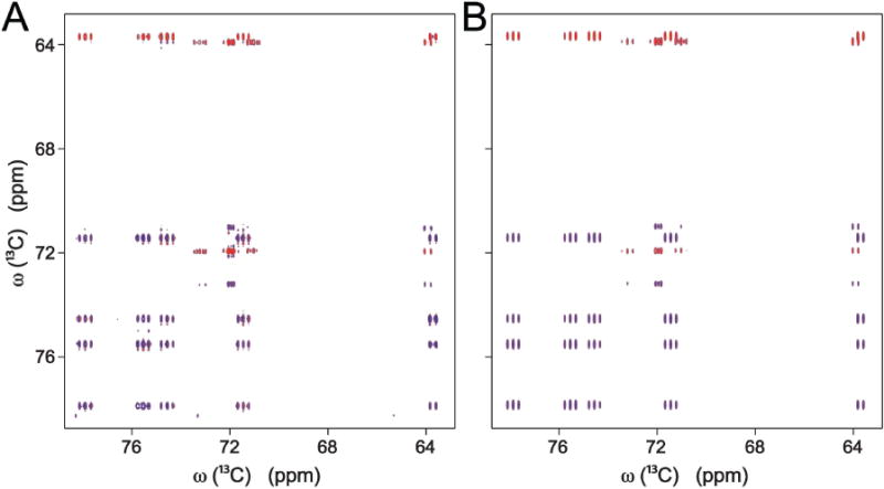
Side-by-side comparison of (A) experimental and (B) simulated 2D 13C–13C constant-time (CT) TOCSY spectrum of galactose acquired at long TOCSY mixing time. Blue colored peaks are positive and red colored peaks are negative. The simulated spectrum, which uses chemical shifts, backbone topology, and 1J(CC) couplings, is based on Eq. (1).
Quantification of carbohydrate mixture
Our compound quantification method using a long mixing time TOCSY spectrum (Method A) was first tested for a carbohydrate mixture consisting of uniformly 13C-labeled ribose, glucose, fructose and galactose. In aqueous solution, each of these carbohydrates is present in multiple isomeric forms, which are in slow exchange: 2 isomers in the case of galactose and glucose and three isomers in the case of fructose and ribose. Long mixing time CT-TOCSY simulations were performed for each sugar isomer. In the simulated spectra, the peak integrals of each sugar isomer were measured and plotted against the peak integrals of the experimental mixture spectrum. The results for 4 of the sugar isomers are plotted in Figure 2 (first row panels a,b,c,d) and the spectra of all sugar isomers are given in Figure S-2. As can be seen from the figure, the experimental and computed peak integrals align well along the diagonal with a correlation coefficient R between 0.92 and 0.98. For the plots, the experimental peak amplitudes were normalized such that the points lie along the main diagonal. The relative concentrations of the various isomers are indicated by the constant a given in each panel, which correspond to the actual slopes. Consistently good results are obtained for all peaks with the exception of peaks whose donor carbon frequency exceeds 100 ppm. This behavior is presumably caused by the larger radio-frequency offset effects and they were excluded from analysis (and are not shown in the figures). Overlapping diagonal peaks were also excluded.
Figure 2.
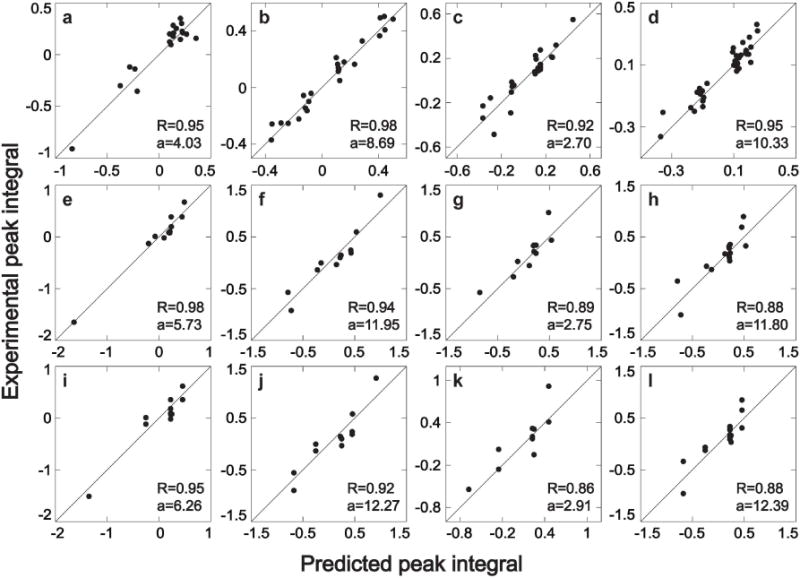
Quantitative comparison of experimental and simulated cross-peak integrals of 2D 13C–13C constant-time (CT) TOCSY of four different carbohydrates. Panels a, e, i belong to fructose β-furanose, panels b, f, j belong to glucose β-pyranose, panels c, g, k belong to ribose β-furanose, and panels d, h, l belong to galactose β-pyranose. The first row of panels (a, b, c, d) shows the comparison between experimental long mixing-time CT-TOCSY (τm = 47 ms) and numerical simulation based on Eq. (1) (Method A). The second row of panels (e, f, g, h) shows the comparison between experimental short mixing-time CT-TOCSY (τm = 4.7 ms) and numerical simulation based on Eq. (1) (Method B). The third row of panels (i, j, k, l) shows the comparison between experimental short mixing-time CT-TOCSY (τm = 4.7 ms) and numerical results using the analytical approximations (Method C). R and a, which are listed in each panel, stand for correlation coefficient and relative concentration, respectively.
A distinctive feature of long-mixing CT-TOCSY is the large number of cross-peaks as the number of peaks grows with the square of the chain length. For example, for a linear 6-carbon chain, such as α-glucose, the total number of cross-peaks and diagonal peaks is 36. Even in the case of some overlaps, the number of peaks available for quantification of the compound is therefore large. It not only helps reduce the statistical uncertainty, but it also allows identification of ‘outliers’, which includes peaks whose volumes are affected by spectral artifacts, and thereby increases the confidence and precision of the concentration estimates.
The same procedure used for the analysis of the long-mixing CT-TOCSY spectra was applied to short mixing time CT-TOCSY (Method B). The results for 4 of the carbohydrate isomers are plotted in Figure 2e,f,g,h and the results for all sugar isomers are shown in Figure S-3. The correlation coefficients between computed and experimental peak volumes vary between 0.88 and 0.98. The short-mixing CT-TOCSY has significantly fewer cross-peaks than the long-mixing TOCSY as the number of peaks grows linearly with the chain length. For example, for a linear 6-carbon chain, such as α-glucose, the total number of peaks is 16.
At long mixing times, analytical solutions do not exist for all but the simplest spin systems. On the other hand, for sufficiently short mixing time, the exact transfer amplitudes can be empirically approximated as shown in the Methods section (Method C). The accuracy of these approximations can be assessed in Figures 2i,j,k,l and S-4 where the approximate peak volumes at 4.7 ms mixing time are compared with the experimentally extracted volumes at the same mixing time. The correlation coefficients vary between 0.86 and 0.95, which is very similar to the performance of the exact treatment at short mixing times (Method B).
Carbohydrate isomer population determination
The ability to accurately determine the populations of each isomer of a given carbohydrate is a useful indicator for the accuracy of the different methods. For this purpose, the relative isomer populations determined by 5 different methods are compared in Table 1. Two of these methods are based on a 1D 13C NMR spectrum of either a sample of a pure compound or the 1D 13C NMR spectra of the mixture. The other 3 approaches use 2D CT-TOCSY information according to Methods A, B, C. In the case of galactose, Method A yields populations of its two isomers α-pyranose and β-pyranose of 35.3% and 64.7%, respectively. These percentages are close to the ones observed in 1D 13C NMR spectra of individual galactose (33.3% vs. 66.7%) as well as galactose peaks in 1D 13C NMR spectra of the carbohydrate mixture (33.2% vs. 66.8%). Methods B and C, which rely on short-mixing CT-TOCSY, yield results with larger deviations (Method B: 36.2% vs. 63.8% and Method C: 28.1% vs. 71.9%). This is primarily due to the smaller number of peaks leading to larger statistical errors and distorted peak shapes caused by the presence of zero-quantum effects. Overall, the 5 methods produce consistent results for both galactose and glucose. For the other 2 carbohydrates, which both have at least one isomer with notably low concentration (<20%), fructose isomer concentrations were determined quite accurately by Method A. Ribose isomer concentrations could be determined less accurately by all three methods, since peaks of the high-population isomer β-pyranose and the low-population isomer α-pyranose overlap throughout the spectrum. Taken together, the long-mixing TOCSY (Method A) produces somewhat more robust population estimates as judged by their better agreement with the 1D methods than the short-mixing TOCSY.
Table 1.
Quantification results for carbohydrate mixture.
| Aa | Bb | Cc | 1D Mixtured | 1D Individuale | |
|---|---|---|---|---|---|
| galactose β-pyranose | 64.7 % | 63.8 % | 71.9 % | 66.8 % | 66.7 % |
| galactose α-pyranose | 35.3 % | 36.2 % | 28.1 % | 33.2 % | 33.3 % |
| glucose β-pyranose | 58.8 % | 61.8 % | 61.3 % | 63.3 % | 62.5 % |
| glucose α-pyranose | 41.2 % | 38.2 % | 38.7 % | 36.7 % | 37.5 % |
| fructose β-furanose | 20.0 % | 22.3 % | 22.4 % | 21.6 % | 24.2 % |
| fructose β-pyranose | 72.8 % | 52.8 % | 50.7 % | 70.5 % | 69.4 % |
| fructose α-furanose | 7.2 % | 24.9 % | 26.9 % | 7.9 % | 6.4 % |
| ribose β-furanose | 18.2 % | 14.1 % | 14.5 % | 13.0 % | 12.9 % |
| ribose β-pyranose | 69.2 % | 69.9 % | 69.6 % | 80.6 % | 80.4 % |
| ribose α-furanose | 12.6% | 16.0 % | 15.9 % | 6.4 % | 6.7 % |
Results when Method A is used for quantification.
Results when Method B is used for quantification.
Results when Method C is used for quantification.
Quantification from 1D 13C NMR spectrum of carbohydrate mixture.
Quantification from 1D 13C NMR spectra of individual carbohydrates.
Quantification of amino-acid mixture
This sample consists of an aqueous mixture of isoleucine, lysine, alanine and valine with concentrations of 5, 10, 15 and 20 mM, respectively. Long-mixing CT-TOCSY simulations were performed for each amino acid (Method A). From the simulated spectra, peak integrals were extracted and plotted against the corresponding peak integrals of the experimental mixture spectrum (Figure 3a,b,c,d). Peaks whose donor carbon is a Cα gave relatively large errors and they were excluded from analysis. The correlation coefficients lie between 0.83 (valine) and 0.98 (isoleucine).
Figure 3.
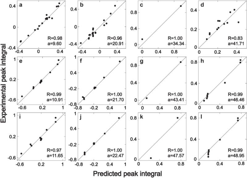
Quantitative comparison of experimental and simulated cross-peak integrals of 2D 13C–13C constant-time (CT) TOCSY of four different amino acids. Panels a, e, i belong to isoleucine, panels b, f, j belong to lysine, panels c, g, k belong to alanine, and panels d, h, l belong to valine. The first row of panels (a, b, c, d) shows the comparison between experimental long mixing-time CT-TOCSY (τm = 47 ms) and numerical simulation based on Eq. (1) (Method A). The second row of panels (e, f, g, h) shows the comparison between experimental short mixing-time CT-TOCSY (τm = 4.7 ms) and numerical simulation based on Eq. (1) (Method B). The third row of panels (i, j, k, l) shows the comparison between experimental short mixing-time CT-TOCSY (τm = 4.7 ms) and numerical results using the analytical approximations (Method C). R and a, which are listed in each panel, stand for correlation coefficient and relative concentration, respectively.
The results for the short-mixing TOCSY (Method B) is shown in Figure 3e,f,g,h with correlation coefficients between 0.99 and 1.00. The relative concentration of isoleucine, lysine and valine can be obtained with reasonably high accuracy. Only for alanine, for which only 2 peaks were used, severe peak distortions leads to a worse performance than for long-mixing CT-TOCSY. The same conclusions hold for the approximate treatment of the short-mixing TOCSY (Method C) with the results shown in Figure 3i,j,k,l.
The concentration ratios of the amino acids were extracted from Figure 3 and with the results listed in Table 2. They show that the relative concentrations of isoleucine, lysine and valine can be obtained with high accuracy by all 3 methods. For alanine with only 2 cross-peaks, and hence poorer statistics, the accuracy is clearly lower.
Table 2.
Quantification results for amino acid mixture.
| Aa | Bb | Cc | 1D Mixtured | Gravimetrice | |
|---|---|---|---|---|---|
| Isoleucine | 1.00x | 1.00x | 1.00x | 1.00x | 1.00x |
| Lysine | 2.18x | 1.99x | 1.93x | 2.07x | 2.00x |
| Alanine | 3.58x | 3.98x | 4.08x | 2.94x | 3.00x |
| Valine | 4.34x | 4.26x | 4.20x | 4.10x | 4.00x |
Results when Method A is used for quantification.
Results when Method B is used for quantification.
Results when Method C is used for quantification.
Quantification from 1D 13C NMR spectrum of amino acid mixture.
Relative amino acid concentrations when amino acid mixture was prepared.
Concluding Remarks
Identification and quantification of metabolites in complex mixtures is a key challenge of metabolomics. Quantification of components by NMR spectroscopy is traditionally based on peak integrals of 1D NMR spectra. This method can provide very accurate concentration estimates, but it is limited to spectra with relatively little peak overlap. For complex metabolite mixtures, such as the ones encountered in metabolomics, peak overlaps in the 1D spectrum are typically prevalent to the extent that they significantly hamper or prevent the use of 1D spectra for quantification. Although the overlap issue can be addressed by taking advantage of the substantial resolution enhancement offered by 2D NMR spectra, magnetization transfers during 2D experiments lead to non-uniform scaling across the spectrum, which impairs the direct proportionality relationship between peak volumes and compound concentration. The course of magnetization transfer in 2D 13C–13C CT-TOCSY experiment is however complex especially at longer mixing times. This experiment is ideally suited for the study of uniformly 13C-labeled organisms, such as bacteria, yeast, and plants, permitting the ab initio determination of the carbon-backbone topologies of sizeable numbers of known and unknown metabolites.14 We demonstrate here that this experiment cannot only be used for metabolite identification, but also for quantification purposes provided that the dependence of the cross-peak amplitudes on the mixing time is explicitly taken into account. This can be achieved either through the explicit quantum-mechanical treatment of the underlying spin physics at arbitrary TOCSY mixing times or, in case of short mixing times, by the use of the analytical expressions presented here. Our results for carbohydrates and amino acids show that at long mixing times, the fully quantum-mechanics based calculation of magnetization transfer during TOCSY well reproduces the experimental observations. At shorter mixing times, the accuracy is slightly reduced because of the smaller number of amenable cross-peaks and potentially distorted peak shapes. The achievable accuracy by the 2D CT-TOCSY-based approach is not as high as for the traditional 1D 1H NMR approach. However, the use of CT-TOCSY for compound quantification overcomes the need of well-resolved resonances in the 1D NMR spectrum. Application of this quantification method to 1H–1H TOCSY spectra is possible, but it requires accurate knowledge of all geminal and vicinal J(1H, 1H) couplings, which can strongly depend on the metabolite conformation(s). On the other hand, since 13C CT-TOCSY approach is 13C-based during both evolution and detection, it does neither require any 1H resonance assignments nor knowledge of J(1H, 1H)-couplings. It can be applied to the very same 13C–13C TOCSY spectra used for compound identification and backbone-carbon topology reconstruction. Moreover, the protocol should be applicable to fractionally 13C-labeled metabolites, such as ones used for flux analysis, provided that cross-peaks of differentially labeled variants of the same molecule do not overlap to an extent that might hinder the accurate measurement of individual cross-peak volumes. These properties make CT-TOCSY spectra a powerful tool for metabolomics studies of 13C-labeled organisms that aim at compound identification and quantification.
Supplementary Material
Acknowledgments
This work was supported by the National Institutes of Health (grant R01 GM 066041).
Footnotes
Supporting Information Available: This material is available free of charge via the Internet at http://pubs.acs.org.
References
- 1.Lenz EM, Wilson ID. J Proteome Res. 2007;6:443–458. doi: 10.1021/pr0605217. [DOI] [PubMed] [Google Scholar]
- 2.Robinette SL, Brüschweiler R, Schroeder FC, Edison AS. Acc Chem Res. 2012;45:288–297. doi: 10.1021/ar2001606. [DOI] [PMC free article] [PubMed] [Google Scholar]
- 3.Pauli GF, Jaki BU, Lankin DC. J Nat Prod. 2005;68:133–149. doi: 10.1021/np0497301. [DOI] [PubMed] [Google Scholar]
- 4.Shaykhutdinov RA, MacInnis GD, Dowlatabadi R, Weljie AM, Vogel HJ. Metabolomics. 2009;5:307–317. [Google Scholar]
- 5.Pauli GF, Godecke T, Jaki BU, Lankin DC. J Nat Prod. 2012;75:834–851. doi: 10.1021/np200993k. [DOI] [PMC free article] [PubMed] [Google Scholar]
- 6.Lewis IA, Schommer SC, Hodis B, Robb KA, Tonelli M, Westler WM, Sussman MR, Markley JL. Anal Chem. 2007;79:9385–9390. doi: 10.1021/ac071583z. [DOI] [PMC free article] [PubMed] [Google Scholar]
- 7.Gronwald W, Klein MS, Kaspar H, Fagerer SR, Nurnberger N, Dettmer K, Bertsch T, Oefner PJ. Anal Chem. 2008;80:9288–9297. doi: 10.1021/ac801627c. [DOI] [PubMed] [Google Scholar]
- 8.Gowda GAN, Tayyari F, Ye T, Suryani Y, Wei SW, Shanaiah N, Raftery D. Anal Chem. 2010;82:8983–8990. doi: 10.1021/ac101938w. [DOI] [PMC free article] [PubMed] [Google Scholar]
- 9.Martineau E, Tea I, Akoka S, Giraudeau P. NMR Biomed. 2012;25:985–992. doi: 10.1002/nbm.1816. [DOI] [PubMed] [Google Scholar]
- 10.Rai RK, Tripathi P, Sinha N. Anal Chem. 2009;81:10232–10238. doi: 10.1021/ac902405z. [DOI] [PubMed] [Google Scholar]
- 11.Koskela H, Heikkila O, Kilpelainen I, Heikkinen S. J Magn Reson. 2010;202:24–33. doi: 10.1016/j.jmr.2009.09.021. [DOI] [PubMed] [Google Scholar]
- 12.Hu K, Westler WM, Markley JL. J Am Chem Soc. 2011;133:1662–1665. doi: 10.1021/ja1095304. [DOI] [PMC free article] [PubMed] [Google Scholar]
- 13.Rai RK, Sinha N. Anal Chem. 2012;84:10005–10011. doi: 10.1021/ac302457s. [DOI] [PubMed] [Google Scholar]
- 14.Bingol K, Zhang F, Bruschweiler-Li L, Brüschweiler R. J Am Chem Soc. 2012;134:9006–9011. doi: 10.1021/ja3033058. [DOI] [PMC free article] [PubMed] [Google Scholar]
- 15.Cavanagh J, Chazin WJ, Rance M. J Magn Reson. 1990;87:110–131. [Google Scholar]
- 16.Brüschweiler R, Ernst RR. J Magn Reson. 1997;124:122–126. doi: 10.1006/jmre.1998.1368. [DOI] [PubMed] [Google Scholar]
- 17.Butler MC, Dumez J-N, Emsley L. Chem Phys Lett. 2009;477:377–381. [Google Scholar]
- 18.Eletsky A, Moreira O, Kovacs H, Pervushin K. J Biomol NMR. 2003;26:167–179. doi: 10.1023/a:1023572320699. [DOI] [PubMed] [Google Scholar]
- 19.Braunschweiler L, Ernst RR. J Magn Reson. 1983;53:521–528. [Google Scholar]
- 20.Bingol K, Brüschweiler R. Anal Chem. 2011;83:7412–7417. doi: 10.1021/ac201464y. [DOI] [PMC free article] [PubMed] [Google Scholar]
- 21.Bingol K, Zhang F, Bruschweiler-Li L, Brüschweiler R. Anal Chem. 2012;84:9395–9401. doi: 10.1021/ac302197e. [DOI] [PMC free article] [PubMed] [Google Scholar]
- 22.Azurmendi HF, Freedberg DI. J Magn Reson. 2013;228:130–135. doi: 10.1016/j.jmr.2013.01.001. [DOI] [PubMed] [Google Scholar]
- 23.Kadkhodaie M, Rivas O, Tan M, Mohebbi A, Shaka AJ. J Magn Reson. 1991;91:437–443. [Google Scholar]
- 24.Delaglio F, Grzesiek S, Vuister GW, Zhu G, Pfeifer J, Bax A. J Biomol NMR. 1995;6:277–293. doi: 10.1007/BF00197809. [DOI] [PubMed] [Google Scholar]
Associated Data
This section collects any data citations, data availability statements, or supplementary materials included in this article.