

Summary
Single-particle cryogenic electron microscopy (cryo-EM) is a powerful tool for the study of macromolecular structures at high resolution. Classification allows multiple structural states to be extracted and reconstructed from the same sample. One classification approach is via the covariance matrix, which captures the correlation between every pair of voxels. Earlier approaches employ computing-intensive resampling and estimate only the eigenvectors of the matrix, which are then used in a separate fast classification step. We propose an iterative scheme to explicitly estimate the covariance matrix in its entirety. In our approach, the flexibility in choosing the solution domain allows us to examine a part of the molecule in greater detail. 3D covariance maps obtained in this way from experimental data (cryo-EM images of the eukaryotic pre-initiation complex) prove to be in excellent agreement with conclusions derived by using traditional approaches, revealing in addition the interdependencies of ligand bindings and structural changes.
Introduction
Recent developments of single-particle cryo-electron microscopy have attracted a great deal of attention in the structural biology community (Campbell, et al., 2012; Li, et al., 2013; Bai, et al., 2013), due to the ability of this technique to achieve near-atomic resolution for biological macromolecules that are imaged in a near-native environment. In the single-particle method, two-dimensional (2D) noisy projections of macromolecules lying in random orientations are collected in the electron microscope (Frank, 2006). In many cases several conformations and binding states coexist. To deal with the resulting heterogeneity in the sample, several methods have been proposed, ranging from earlier approaches based on clustering of 2D projections (e.g., (Van Heel & Frank, 1981)) to more recently developed three-dimensional (3D) approaches. Maximum-likelihood-based techniques assume a probability distribution over the projections, given a small and known number of discrete classes (Sigworth, et al., 2010; Scheres, 2010; Lee, et al., 2011; Wang, et al., 2013). Statistical bootstrapping methods (Simonetti, et al., 2008; Spahn & Penczeck, 2009; Liao & Frank, 2010; Penczek, et al., 2011) estimate the 3D covariance matrix of the underlying molecules indirectly. Following this approach, a large number of reconstructions are created from the data by resampling, and the projections are represented in a low-dimensional space spanned by the projections of the top eigenvolumes of the bootstrap reconstructions. That is, instead of the covariance matrix itself, bootstrapping methods estimate the top-ranking eigenvolumes, which are also the top eigenvectors of the covariance matrix. Typically, only a small number of eigenvectors are estimated (e.g., less than fifteen in the work by (Penczek, et. al. 2011)). In principle, the covariance matrix can be obtained by combining all the estimated eigenvector (or approximated by a subset of the dominant eigenvectors), weighted by their respective energies. However, due to the errors in the estimation, the covariance matrix may not be reliably and efficiently obtained in this way. Classification is then achieved by clustering the projections represented in the low-dimensional space. Other classification methods that have been proposed are based on graph-theory and common lines (Herman & Kalinowski, 2008; Shatsky, et al., 2010), as well as stochastic climbing (Tang, et al., 2007; Elmlund, et al., 2013).
All existing reference-free classification algorithms are highly computing-intensive. They do a good job at separating different conformations or binding states when those differences are large. However, this is not the case when the differences are small (e.g., presence versus absence of small ligands), due to the low signal-to-noise-ratio of the projection data, which in turn precludes an accurate determination of the projection angles, exacerbating the separation task. Hence, there is interest in studying the case of small and localized differences; and we believe this is where our approach can make a significant contribution. It should be pointed out that when the sample contains a continuous range of conformations, the assumption of a discrete number of classes (a tenet of all classification algorithms currently in use) is no longer adequate, leaving room for approaches, such as (Dashti, et al., 2014), which is capable of mapping continuous conformational changes based on manifold embedding.
At this point we would like to emphasize a property of the covariance matrix that goes beyond classification, which has received little attention: the determination of interdependencies in the study of molecules with multiple binding partners (ligands). An example is provided by the recent study of the eukaryotic pre-initiation complex (Hashem, et al., 2013) whose assembly involves the processive interaction between the 40S subunit, initiator tRNA and several initiation factors. Here the presence of a factor might be favored by the absence of another. Binding of a factor might induce the movement of a subunit domain. The study of all such contingencies is facilitated by computing relevant portions of the covariance matrix from a heterogeneous sample. By definition, the entry at row i and column j of the covariance matrix records the covariance between the values in two voxels with indices i and j, respectively. The i-th row of the matrix thus contains the covariances between voxel i and all the voxels. These numbers can thus be arranged in 3D and visualized as a volume, which we refer to as the covariance map with respect to voxel i, and this voxel is referred to as the reference voxel for this map. A similar concept of the covariance map applies to images, by simply replacing the word “voxel” by “pixel” and “volume” by “image.” When the reference voxel lies inside a ligand, this map will indicate how strongly the presence of this ligand correlates with the presence of other ligands and with structural changes in the molecule the ligands are bound to. That is, all the interdependencies with a ligand are revealed in one single map. As a byproduct, the shape of the ligands and the trace of continuous conformational changes are also brought out.
When the assumption of a discrete number of classes is valid, Penczek et al. (Penczek, et al., 2011) showed that the eigenvectors of the covariance matrix reveal the structures of the conformers. For example, in the simple case of two classes in which the only difference is that a small ligand is present within one but not the other, the first eigenvolume will be proportional to the density of this ligand only; i.e., the eigenvolume has high values in a region that has the shape of the ligand. In fact, the covariance matrix itself also reflects the structure of the ligand in this case: since the elements of this matrix record the covariance between every pair of voxels, the covariance between a voxel lying in one of the ligands and another voxel is respectively, positive, negative, or zero, depending on whether the second voxel is within the same ligand, within a different ligand, or in the remaining space. In contrast, when there is a continuous range of conformations in the sample, we will show below that the trajectory of this continuous change will be reflected in the covariance map but not in the eigenvolumes.
In this paper, we are concerned with estimating the covariance matrix in an efficient way. Katsevitch et al. (Katsevich, et al., 2014) proposed an elegant way of estimation in the Fourier domain. They computed the eigenvectors of the matrix in the Fourier domain, then Fourier-inverted them to get the eigenvectors back in real space, and finally proceeded with the classification step as in (Spahn & Penczeck, 2009; Penczek, et al., 2011). Resampling is thereby avoided; however, this approach has only been demonstrated on volumes of sizes up to 173. Nevertheless, unlike earlier works, the approach used in (Katsevich, et al., 2014) provides a guarantee that the estimated covariance matrix converges to the true covariance matrix in the limit of infinite number of projection images.
We estimate the whole covariance matrix (not just its eigenvectors) explicitly in real space, and within a domain of arbitrary shape, a feature that is not possible using approaches that solve in Fourier space. Hence, our approach avoids resampling and –more importantly– enables the analysis of the covariance in localized regions. The computational savings resulting from solving the matrix in a few small regions rather than the whole volume allows solutions with higher resolution. In our experiments, the 3D covariance maps are in excellent agreement with conclusions from traditional approaches, as the maps show the interdependencies of sub-stoichiometrically bound ligands and conformational changes they spawn.
In our approach, we solve a system of linear equations in which the unknowns are the entries of the 3D covariance matrix and the right hand side is composed of the covariances derived from the projection data. Linear relationships between the former type of covariance (later referred to as “3D covariance”) and the latter type (later referred to as “2D covariance”) have already been established in (Katsevich, et al., 2014).
Results
Estimation of the covariance
We discretize the volume containing a macromolecule as having N3 voxels and model it as a N3-dimensional vector X. The 3D covariance matrix is defined as follows. If the heterogeneous set of macromolecules are brought into the same coordinate system and the volume containing them is represented by a 3D array of voxels, then the covariance between the values in two voxels x1 and x2 is defined as
| (1) |
where E(.) denotes the expected value. A positive (negative) covariance means that when the value in x1 is above E(x1), then the value in x2 tends to be above (below) E(x2). Given three voxels x1, x2 and x3, if cov(x1, x2) is greater than cov(x1, x3) in absolute value, then a change in the value of x1 implies a bigger change in the value of x2 than in the value of x3.
A projection image from the data is modeled as a noisy approximation to the line integrals across the volume in a given direction, which we write as Y = RX, where R contains the orientation-dependent coefficients in the integrals. When X is random, so is Y; and it can be shown that their respective covariance matrices (after stacking the entries of a matrix to form a column vector) are related by the matrix-vector equation:
| (2) |
where CY is the covariance of the line integrals (to be referred to as “2D covariance”), CX is the unknown covariance (“3D covariance”), and the elements of W are products of elements of R (see Supplemental Information). In practice, many projections exist, and therefore one could concatenate all these equations and solve the entire system. However, for reasons of expediency, we group or bin the projections based on their similarity of orientations and create one equation like Equation 2 for each group (hence one W is given for each group). Our aim is to estimate the 3D covariance from the set of 2D covariances calculated from the projections. Going back to the definition of the covariance matrix: the diagonal entries of this matrix constitute the variance map (Liu & Frank, 1995), and one row (or column, since the matrix is symmetric) of the covariance matrix is referred to as the covariance map with respect to the voxel having that row number. Figure 1 illustrates the estimation principle.
Figure 1.
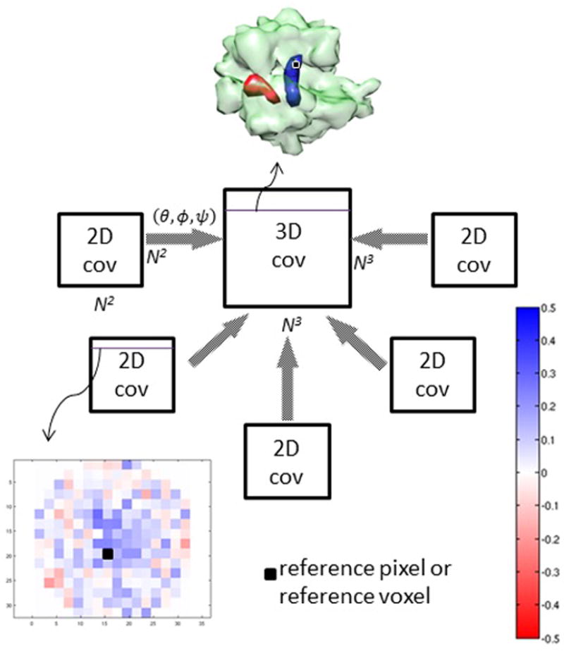
Principle of 3D covariance estimation. The 3D covariance, which is of size N3×N3 where N3 is the size of the volume, is estimated from all the 2D covariances – of size N2×N2 – at different angles (θ,ϕ,ψ). First, the 2D covariances are calculated; each row of a 2D covariance matrix can be depicted as a 2D covariance map (with respect to the pixel with that row number in the covariance matrix), which resembles the red-blue map at the bottom left. Once the 3D covariance is estimated, the row of the matrix corresponding to a voxel of interest can be extracted and represented as a volume like the red-blue map at the center top. In our example, the simulated data consist of identical ribosomes (depicted as green transparent density map) with a ligand bound in one of the two positions (red and blue).
Noise is an important consideration in the estimation. We assume that the noise is additive and statistically independent from structural heterogeneity, but we do not make any assumptions on the type of noise spectrum (Meyer & Kirkland, 1998; Shigematsu & Sigworth, 2013). To correct for the contributions by noise, we subtract the 2D covariance of a pure-noise projection from the corresponding measured 2D covariance (Supplemental Information, Figure S1). We normalize the images by setting the background to zero mean and unit variance to compensate for data imperfections, such as those created by uneven ice thickness or uneven illumination. We assume that the data are correctly aligned and already corrected for the Contrast Transfer Function (CTF) (Frank, 2006).
From the point of view of achievable resolution, the orientation bin size is determined by the Shannon angle, which is defined as the ratio between the resolution (expressed as a distance in real space) and the diameter of the object. Binning, however, creates an unwanted extra variability, which nevertheless can be considerably reduced by subtracting the reprojection of a volume reconstructed from the normalized projection data (Supplemental Information). We found in our experiments that this variability is not significant if we use four degrees or less, which is approximately the Shannon angle corresponding to a volume size of 323, if we consider a resolution of two voxels and a diameter of 32 voxels.
Because the number of unknowns increases quadratically with the number of voxels, for faster computation we perform a preliminary reconstruction using a coarse sampling grid, then another reconstruction of only the region of interest possessing high variability, using a finer grid.
To solve the system of equations, we use an iterative algorithm known as block-ART ((Herman, 1970; Censor & Zenios, 1997) and Supplemental Information). We found that usually twenty or fewer iterations are adequate to obtain a stable solution.
Proof of Principle
Simulated data of the 70S ribosome in two conformations
We first tested our approach on simulated data consisting of 10,000 noiseless 20×20 projections of an E. coli 70S ribosome density map with either a P-site or an A-site tRNA (Figure 2), each of which generating 5,000 projections with an approximately even distribution of orientations. To keep the same orientation bin size throughout the experiments in this paper, we used bins of approximately four degrees, even though the Shannon angle is in this case 2/20 radians = 5.7 degrees. As expected, we observe that (i) high variance occurs only at the places of both tRNAs, (ii) positive covariance between a voxel of high variance (black dot) and all the voxels of the tRNA containing it, and (iii) negative covariance between that same voxel and all the voxels of the other tRNA. Hence we see that the covariance map indicates the interdependency of the two tRNAs, and in particular, their shapes are revealed as well.
Figure 2.
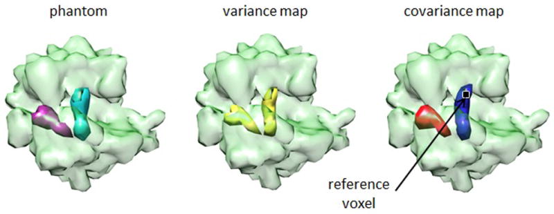
3D Covariance estimation for simulated data. Application of the estimation to a simulated dataset generated from 70S E. coli ribosomes bound with either a P-site tRNA (green) or an A-site tRNA (pink). The panel shows the phantom with the two tRNAs, the calculated variance map, and the covariance map with respect to a voxel of high variance (black dot). Blue (red) color denotes positive (negative) values.
An analysis of continuous conformational change
When it is reasonable to assume that the sample consists of a few classes, both the covariance matrix and its eigenvectors give an insight into the structure of the conformers; this is not the case for continuous conformational changes, however. We show that, while the eigenvectors do not offer an immediate interpretation, useful information can still be reflected in the covariance matrix. To make this point, consider a one-dimensional “volume” (i.e., a vector) of size 11. Assuming that we have a sample with 20 such volumes: ten of them having a “ligand” in the first “voxel” and nothing in the remaining ten voxels; and each one of the other ten volumes contains nothing except a ligand at voxel i, for 2 ≤ i ≤ 11 (see Figure 3 left). With this sample containing 11 classes, we now attempt to approximate a sample whose members have either a ligand, named A, in the first voxel or a ligand, named B, moving continuously anywhere (fractions allowed) between the second and the last voxel; and both ligands never appear simultaneously.
Figure 3.
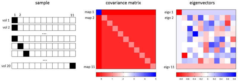
Covariance estimation in the case of approximated continuous conformational change. Left: 20 “volumes” comprising 11 classes. The first class has 10 identical structures has a “ligand” (black square) in the first (left-most) voxel, and the remaining classes (one structure per class) have another ligand at voxel i, for i=2,…,11. Middle: the covariance matrix of these 20 volumes shows a strong negative covariance between voxel 1 and the rest of the voxels. The negative correlation between any two of the remaining voxels is weaker. Each row is the covariance map with respect to the voxel with that row number. Right: each row is an eigenvector of the covariance matrix.
The interdependency of the ligands is clearly mirrored in the covariance matrix (Figure 3 middle): we see a strong negative covariance (−0.5) between the first voxel and any of the remaining ones, and a weaker covariance (−0.05) among the voxels 2 to 11. Each row of the covariance matrix is a covariance map with respect to the voxel with that row number. In order for the map to reveal the “structure,” there has to be a voxel (other than in the diagonal position) with a prominent value. In the example, all the maps corresponding to voxels 2 to 11 highlight the ligand A (at voxel 1). That is, the maps show the structure of ligand A. In contrast, the map corresponding to voxel 1 is uniform across voxels 2 to 11, which means that the map is capturing the trajectory of the ligand B but not its shape. This 11×11 covariance matrix has eigenvalues 5.5, 1, and 0. Because of the multiplicity of eigenvalues, the eigenvectors are not unique, and hence individually they are not informative of this trajectory (Figure 3 right).
Based on this simple example, we conclude that if the shape of a ligand can be identified in the covariance map with respect to a voxel not within the ligand, then there is no continuous motion of the ligand. This is because if there were a continuous motion, a “spreading” of the ligand will be produced, as illustrated in this example.
Covariance maps of a 43S ribosomal pre-initiation complex
Following the encouraging results on simulated data, we next tested our method on experimental data containing 29,000 projections of the mammalian 43S ribosomal pre-initiation complex (Hashem, et al., 2013) (see Figure S2). Pre-initiation complex formation is a key step on the path of translation regulation in eukaryotes. First, the initiator tRNA (Met-tRNAiMet), eukaryotic initiation factor (eIF) 2, and guanosine triphosphate form a ternary complex (TC). The TC, eIF3, eIF1, and eIF1A cooperatively bind to the 40S subunit, yielding the 43S complex, ready to attach to mRNA and scan to the AUG start codon. In addition, the complex was formed in the presence of DHX29, a DExH-box protein that also binds directly to the 40S subunit, required for scanning on structured mRNAs.
The data set was acquired using an FEI Tecnai F20 electron microscope (FEI, Eindhoven) operated at 120 kV with a magnification of 51,570× on a 4k × 4k Gatan Ultrascan 4000 CCD camera with a physical pixel size of 15 μm (thus making the pixel size 2.245 Å). Additional details of sample preparation, data collection and preprocessing can be found below or in ref. (Hashem, et al., 2013). The data were preprocessed using pySPIDER (Robert Langlois and Joachim Frank, unpublished data), yielding a total of ~650,000 particles. Those particles were classified with RELION (Scheres, 2012) and a class of 29,000 particles with all the factors present was isolated.
We chose this data set because we had characterized its structure and wished to see the residual (i.e., after RELION classification) variability in small, localized regions, rather than in large regions. Since the former case tends to be more challenging for most existing classification algorithms, residual variability is likely to be in small regions, and analysis of the covariance enabled by our approach is a promising complementary tool. We found that the covariance maps reveal not only the structure of factors but also their interdependencies. Some results obtained are expected and in excellent agreement with conclusions derived using traditional approaches, and some others are completely new, which opens the door to further investigation.
We first computed the 3D covariance within a sphere inscribed in a cube of 163 voxels. We determined regions of relatively high variance, whose boundaries were then smoothed and used as a new solution domain for recomputing the covariance at higher resolution (of 323 voxels; Figure S3). The Shannon angle in this case is 2/32 radians = 3.6 degrees. The data were grouped using SPIDER command VO EA (Shaikh, et al., 2008) into bins of approximately four degrees, resulting in 1,069 orientation groups, from which we selected the top-620 largest groups. (This cut-off was based on the population size in a bin, which was 12.) We obtained very similar results when we used bin size of approximately 3.3 degrees and 425 largest groups. Computing time was about 4 hours using 12 cores on a 16-core 2.4 GHz AMD Opteron.
The covariance map corresponding to a selected reference voxel in DHX29 (green square, Figure 4 c and d) is seen to capture the structure/shape of the protein itself (green mesh). Since no meaningful negative correlation was observed, the DHX29 molecule in its entirety is likely either present or absent in the class examined. The covariance map corresponding to a voxel (purple square, Figure 4 c and d) in a peripheral subunit of eIF3, unassigned to any specific subunit in our previous work (Hashem, et al., 2013), also captures the shape of the entire subunit. At the same threshold level, it shows a positive correlation with some parts of DHX29. More importantly, both covariance maps show strong positive correlation with a feature corresponding in shape, size and location to eIF3b (Fig. 4 c and d, dashed red oval), consistent with the structure of the complex.
Figure 4.

Covariance analysis of the DHX29-bound 43S Pre-initiation complex (Hashem, et al., 2013). Two covariance maps are shown superimposed with the whole complex. (a) and (b), segmented density map of the DHX29-bound 43S Preinitiation complex. (C) and (d), overlays of covariance maps corresponding to two reference voxels chosen in DHX29 and an unassigned peripheral subunit of eIF3, respectively, showing the DHX29 protein in its entirety (green mesh) and the unassigned peripheral subunit of eIF3 (gray arrow on purple mesh). The latter exhibits positive correlation with parts of DHX29, as demonstrated by the overlapping regions with the map of DHX29. See text.
Figure 5 shows the two maps separately, as well as another map (orange mesh) with respect to a reference voxel in the eIF2-ternary complex (TC, orange square), which reveals the shape of the TC. The map corresponding to DHX29 exhibits a positive correlation with the core of DHX29 (pink arrow) and with the initiator tRNA anti-codon stem-loop (blue arrow). Meanwhile, the map corresponding to TC displays a positive correlation with ribosomal protein S6e (orange arrow). The last two correlations are new findings with potentially important biological implications; thus, additional experiments are required for their elucidations.
Figure 5.

Covariance maps corresponding to voxels in DHX29, a peripheral subunit of eIF3 and eIF2-ternary complex. (a) and (b), the covariance map (purple mesh) of a voxel from the peripheral subunit of eIF3, seen from the solvent side and the front, respectively. The covariance displays clear positive correlation with DHX29 as exemplified by the overlapping of the map with the location of the core of DHX29 (green arrow). (c) and (d), covariance map (green mesh) of a voxel from DHX29, seen from the solvent side and the front, respectively. The covariance map reflects perfectly the shape of DHX29 including its intersubunit domain (pink arrow). Furthermore, the map reveals strong correlation with two regions of the 43S complex corresponding to the location of the initiator tRNA anti-codon stem-loop (panel d, blue arrow). (e) and (f), covariance map (orange mesh) of a voxel from the eIF2-ternary complex (TC), seen from the solvent side and the front, respectively. The covariance reflects the shape of the TC and shows strong positive correlation with the ribosomal protein S6e (panel e and f, orange arrow).
The nature of the positive correlation between ternary complex and eS6 is unclear. It is known that eS6 plays an important role in translation regulation by phosphorylation in response to a wide variety of stimuli on five evolutionarily conserved serine residues. Indeed, eS6 is phosphorylated in yeast and humans and is a target of the mTOR (mammalian target of rapamycin) pathway (Meyuhas, 2008). Phosphorylation in response to mTOR signaling occurs at conserved serines near the C-terminus of the protein (Meyuhas, 2008). The role of this phosphorylation is not well understood but it might be involved in fine-tuning protein translation. Interestingly, the ternary complex can also be phosphorylated on eIF2-α subunit in response to stress --see (Baird & Wek, 2012) for review on eIF2 phosphorylation. The eIF2 phosphorylation regulation pathway is cross-regulated with other regulation pathways such as mTOR. Thus, we hypothesize that the observed correlation between eS6 and the ternary complex may reflect the cross-regulation of phophorylation in response to stress.
We note that in all cases the shapes of the ligands were delineated in the 3D covariance. Hence, no continuous motion was observed.
Discussion
In single-particle cryo-EM data, heterogeneity is an important resolution-limiting factor. One way of studying heterogeneity is via the covariance matrix, which shows regions of high variability (the variance map), as well as the way the value in a given voxel correlates with the remaining ones. While it is mathematically straightforward to estimate this matrix from the covariance of the projections, the rapidly growing number of unknowns as the volume size increases constitutes a big hurdle. This is the reason why solutions have been obtained to date for only relatively small volumes, or strongly decimated versions of larger volumes. In contrast, the flexibility in choosing the size and shape of the solution domain in our approach allows us to deal with volumes in less decimated or undecimated form.
Since the data are not perfect, any type of covariance other than that due to structure variability will be reflected in the results. Therefore, to obtain correct maps, the undesired variability needs to be removed or reduced by proper spatial alignment of the data, statistical considerations, and data normalization. Everything else being equal, we think the signal-to-noise ratio of the data is key to a successful high-resolution estimation of the maps.
We were able to efficiently estimate the covariance matrix and perform a covariance analysis of a 43S pre-initiation complex with DHX29 bound. Images like the ones we used, which correspond to ribosomal complexes imaged under FEI Tecnai electron microscopes and CCD camera, were shown to have a signal-to-noise ratio of approximately 0.1 (Baxter, et al., 2009). Thus, our technique works for this signal-to-noise ratio or higher. With the improved detectors (Campbell, et al., 2012; Li, et al., 2013; Bai, et al., 2013), however, analysis of lighter-weight macromolecules should be feasible, as long as the region of analysis is not too small compared to a voxel (to be safe, the size should be at least 2×2×2 voxels).
Using a coarse sampling grid followed by a finer grid focused on smaller regions of interest has the potential danger that some regions of high variability may be too small to be detected by the initial coarse-grid solution. In this case, an alternative way of locating these small regions is needed prior to the fine-grid computation.
Here we chose to solve the estimation problem iteratively and purely in the image domain. Even though we are not taking advantage of the central slice theorem and applying the fast Fourier transform, we can impose linear or nonlinear constraints directly on the solution, and we could also employ a solution domain of arbitrary shape and size in order to reduce the number of unknowns. Without a proper adjustment of the 2D covariance, however, this strategy implicitly assumes that the variance outside the domain is negligible. If this is not the case, one could tessellate the outside region using larger voxels and include them in the solution domain. We are currently experimenting with these variants, as well as with different types of constraints on the solution, such as smoothness and sparsity.
We are currently developing a python-based software package that implements our proposed technique, which we expect to release it in a couple of months.
Experimental Procedures
Preparation of the 43S Ribosomal Pre-initiation Complex and Its Structure Determination
The complex was prepared as previously described in (Hashem, et al., 2013). In brief, the sample was frozen and applied holey carbon grids (carbon-coated Quantifoil 2/4 grid, Quantifoil Micro Tools GmbH) containing an additional continuous thin layer of carbon (Grassucci, et al., 2007). Grids were blotted and vitrified by rapidly plunging into liquid ethane at −180°C with a Vitrobot (FEI) (Dubochet, et al., 1988; Wagenknecht, et al., 1988). Data acquisition was done under low-dose conditions (12 e−/Å2) on a FEI Tecnai F20 electron microscope (FEI, Eindhoven) operating at 120 kV with a Gatan 914 side-entry cryo-holder. The data set was collected with the automated data collection system Leginon (Suloway, et al., 2005) at a calibrated magnification of 51,5703 on a 4k × 4k Gatan Ultrascan 4000 CCD camera with a physical pixel size of 15mm, thus making the pixel size 2.245 Å on the object scale.
The data were preprocessed using pySPIDER within the Arachnid software package (Robert Langlois and Joachim Frank, unpublished). PySIPDER is a Python-encapsulated version of SPIDER (Leith, et al., 2012; Shaikh, et al., 2008), replacing its batch files with Python scripts. It also contains procedures such as Autopicker (Langlois, et al., 2014), which was used for the automated particle selection, yielding a total number of particles of 650,000. Those particles were classified with RELION (Scheres, 2012) and a class of 29,000 particles with all factors present was isolated. This class was further refined to a resolution of 11.6 Å, as estimated following the “gold-standard” protocol, with a cutoff Fourier shell correlation (FSC) = 0.143 (Henderson, et al., 2012; Scheres, 2012).
3D Covariance Estimation
3D covariance was estimated from the 2D covariances using Equation 2 (see also Figure 1). To estimate the 2D covariances (see Figure S1), we first adjusted the projection images by normalizing them (i.e., setting the background to zero mean and unit variance) and subtracting the reprojection of a volume reconstructed from the normalized data. With the alignment parameters from RELION, we grouped the adjusted data based on their similarity of orientations (with bin size of approximately four degrees) and estimated the covariance for each group. A similar procedure was used to estimate the covariance of noise-only data. Noise-only projections were obtained by shifting each projection by one-half of its size in both vertical and horizontal direction. For each group, the difference between the two covariances is the estimated 2D covariance.
For the simulated data, we computed the 3D covariance within a sphere inscribed in a cube of 203 voxels (Figure 2). For the 43S ribosomal data (Figure S2), the resolution was first 163 voxels. We then determined regions of relatively high variance, whose boundaries were then smoothed and used as a new solution domain (Figure S3) for recomputing the 3D covariance at a resolution of 323 voxels (Figures 4 and 5).
The computations were implemented primarily in MATLAB and SPIDER. We pre-calculated and stored the coefficients of the system of Equation S4. SPIDER was used for the normalization, volume reconstruction, and reprojection (see Equation S1). The remaining steps were implemented in MATLAB and run on a 16-core 2.4 GHz AMD Opteron with 120 Gb memory. The most time-consuming step is to solve Equation S4, which has not been parallelized. A GPU implementation of this step should speed up the estimation process considerably.
Supplementary Material
Acknowledgments
We thank Amedee des Georges for help with the interpretation of the maps and Bob Grassucci for help with the use of UCSF Chimera. This work was supported by HHMI and NIH R01 GM29169 (to J.F.).
References
- Baird T, Wek R. Eukaryotic initiation factor 2 phosphorylation and translational control in metabolism. Adv Nutr. 2012;3(3):307–321. doi: 10.3945/an.112.002113. [DOI] [PMC free article] [PubMed] [Google Scholar]
- Bai X-C, Fernandez IS, McMullan G, Scheres SHW. Ribosome structures to near-atomic resolution from thirty thousand cryo-EM particles. eLife. 2013;2 doi: 10.7554/eLife.00461. [DOI] [PMC free article] [PubMed] [Google Scholar]
- Baxter W, Grassucci R, Gao H, Frank J. Determination of signal-to-noise ratios and spectral SNRs in cryo-EM low-dose imaging of molecules. J Struct Biol. 2009;166(2):126–132. doi: 10.1016/j.jsb.2009.02.012. [DOI] [PMC free article] [PubMed] [Google Scholar]
- Campbell MG, et al. Movies of ice-embedded particles enhance resolution in electron cryo-microscopy. Structure. 2012;20(11):1823–1828. doi: 10.1016/j.str.2012.08.026. [DOI] [PMC free article] [PubMed] [Google Scholar]
- Censor Y, Zenios SA. Parallel Optimization: Theory, Algorithms, and Applications. New York: Oxford University Press; 1997. [Google Scholar]
- Dashti A, et al. Trajectories of the ribosome as a Brownian nanomachine. PNAS. 2014;111:17492–17497. doi: 10.1073/pnas.1419276111. [DOI] [PMC free article] [PubMed] [Google Scholar]
- Dubochet J, et al. Cryo-electron microscopy of vitrified specimens. Q Rev Biophys. 1988;21:129–228. doi: 10.1017/s0033583500004297. [DOI] [PubMed] [Google Scholar]
- Elmlund H, Elmlund D, Bengio S. SIMPLE: Software for ab initio reconstruction of heterogeneous single-particles. Structure. 2013;21(8):1299–1306. doi: 10.1016/j.jsb.2012.07.010. [DOI] [PubMed] [Google Scholar]
- Frank J. Three-Dimensional Electron Microscopy of Macromolecular Assemblies: Visualization of Biological Molecules in Their Native State. New York: Oxford University Press; 2006. [Google Scholar]
- Grassucci RA, Taylor DJ, Frank J. Preparation of macromolecular complexes for cryo-electron microscopy. Nat Protoc. 2007;2:3239–3246. doi: 10.1038/nprot.2007.452. [DOI] [PMC free article] [PubMed] [Google Scholar]
- Hashem Y, et al. Structure of the mammalian ribosomal 43S preinitiation complex bound to the scanning factor DHX29. Cell. 2013;153(5):1108–1119. doi: 10.1016/j.cell.2013.04.036. [DOI] [PMC free article] [PubMed] [Google Scholar]
- Henderson R, et al. Outcome of the first electron microscopy validation task force meeting. Structure. 2012;20:205–214. doi: 10.1016/j.str.2011.12.014. [DOI] [PMC free article] [PubMed] [Google Scholar]
- Herman GT. Algebraic Reconstruction Techniques (ART) for Three-dimensional Electron Microscopy and X-ray Photography. J theor Biol. 1970;29:471–481. doi: 10.1016/0022-5193(70)90109-8. [DOI] [PubMed] [Google Scholar]
- Herman GT. Fundamentals of Computerized Tomography. 2. London: Springer; 2009. [Google Scholar]
- Herman GT, Kalinowski M. Classification of heterogeneous electron microscopic projections into homogeneous subsets. Ultramicroscopy. 2008;108(4):327–338. doi: 10.1016/j.ultramic.2007.05.005. [DOI] [PubMed] [Google Scholar]
- Heymann JB, Cardone G, Winkler DC, Steven AC. Computational resources for cryo-electron tomography in Bsoft. J Struct Biol. 2008;161:232–242. doi: 10.1016/j.jsb.2007.08.002. [DOI] [PMC free article] [PubMed] [Google Scholar]
- Katsevich G, Katsevich A, Singer A. Covariance Matrix Estimation for the Cryo-EM Heterogeneity Problem. 2014 doi: 10.1137/130935434. s.l.: arXiv.org. [DOI] [PMC free article] [PubMed] [Google Scholar]
- Langlois R, et al. Automated particle picking for low-contrast macromolecules in cryo-electron microscopy. J Struct Biol. 2014;186:1–7. doi: 10.1016/j.jsb.2014.03.001. [DOI] [PMC free article] [PubMed] [Google Scholar]
- Lee S, Doerschuk P, Johnson JE. Multiclass maximum-likelihood symmetry determination and motif reconstruction of 3-D helical objects from projection images for electron microscopy. IEEE Trans Image Process. 2011;20(7):1962–1976. doi: 10.1109/TIP.2011.2107329. [DOI] [PMC free article] [PubMed] [Google Scholar]
- Leith A, Baxter W, Frank J. Use of SPIDER and SPIRE in Image Reconstruction. In: Arnold E, Himmel D, Rossmann M, editors. International Tables for Crystallography. Crystallography of Biological Macromolecules. New York: John Wiley; 2012. pp. 620–623. [Google Scholar]
- Liao HY, Frank J. Classification by bootstrapping in single particle methods. Amsterdam: ISBI, IEEE; 2010. [DOI] [PMC free article] [PubMed] [Google Scholar]
- Liu W, Frank J. Estimation of variance distribution in three-dimensional reconstruction. I Theory. J Opt Soc Am A. 1995;12(12):2615–2627. doi: 10.1364/josaa.12.002615. [DOI] [PubMed] [Google Scholar]
- Li X, et al. Electron counting and beam-induced motion correction enable near-atomic-resolution single-particle cryo-EM. Nat Methods. 2013;10(6):584–590. doi: 10.1038/nmeth.2472. [DOI] [PMC free article] [PubMed] [Google Scholar]
- Meyer R, Kirkland A. The effects of electron and photon scattering on signal and noise transfer properties of scintillators in CCD cameras used for electron detection. Ultramicroscopy. 1998;75:23–33. [Google Scholar]
- Meyuhas O. Physiological roles of ribosomal protein S6: One of its kind. Int Rev Cell Mol Biol. 2008;268:1–37. doi: 10.1016/S1937-6448(08)00801-0. [DOI] [PubMed] [Google Scholar]
- Penczek PA, Kimmel M, Spahn CMT. Identifying Conformational States of Macromolecules by Eigen-Analysis of Resampled Cryo-EM Images. Structure. 2011;19(11):1582–90. doi: 10.1016/j.str.2011.10.003. [DOI] [PMC free article] [PubMed] [Google Scholar]
- Penczek PA, Yang C, Frank J, Spahn CMT. Estimation of variance in single-particle reconstruction using the bootstrap technique. J Struc Biol. 2006;154:168–183. doi: 10.1016/j.jsb.2006.01.003. [DOI] [PubMed] [Google Scholar]
- Scheres SHW. Classification of structural heterogeneity by maximum-likelihood methods. Meth Enzym. 2010;482:295–320. doi: 10.1016/S0076-6879(10)82012-9. [DOI] [PMC free article] [PubMed] [Google Scholar]
- Scheres SHW. A Bayesian view on cryo-EM structure determination. J Mol Biol. 2012;415:406–418. doi: 10.1016/j.jmb.2011.11.010. [DOI] [PMC free article] [PubMed] [Google Scholar]
- Shaikh TR, et al. SPIDER image processing for single-particle reconstruction of biological macromolecules from electron micrographs. Nat Protoc. 2008;3:1941–1974. doi: 10.1038/nprot.2008.156. [DOI] [PMC free article] [PubMed] [Google Scholar]
- Shatsky M, et al. Automated multi-model reconstruction from single-particle electron microscopy data. J Struct Biol. 2010;170(1):98–108. doi: 10.1016/j.jsb.2010.01.007. [DOI] [PMC free article] [PubMed] [Google Scholar]
- Shigematsu H, Sigworth F. Noise models and cryo-EM drift correction with a direct-electron camera. Ultramicroscopy. 2013;131:61–69. doi: 10.1016/j.ultramic.2013.04.001. [DOI] [PMC free article] [PubMed] [Google Scholar]
- Sigworth FJ, Doerschuk PC, Carazo JM, Scheres SHW. An introduction to maximum-likelihood methods in cryo-EM. Methods Enzymol. 2010;482:263–294. doi: 10.1016/S0076-6879(10)82011-7. [DOI] [PMC free article] [PubMed] [Google Scholar]
- Simonetti A, et al. Structure of the 30S translation initiation. Nature. 2008;455:416–420. doi: 10.1038/nature07192. [DOI] [PubMed] [Google Scholar]
- Spahn CMT, Penczeck PA. Exploring conformational modes of macromolecular assemblies by multi-particle cryo-EM. Curr Opin Struct Biol. 2009;19(5):623–631. doi: 10.1016/j.sbi.2009.08.001. [DOI] [PMC free article] [PubMed] [Google Scholar]
- Suloway C, et al. Automated molecular microscopy: the new Leginon system. J Struct Biol. 2005;151:41–60. doi: 10.1016/j.jsb.2005.03.010. [DOI] [PubMed] [Google Scholar]
- Tang G, et al. EMAN2: an extensible image processing suite for electron microscopy. J Struct Biol. 2007;157:38–46. doi: 10.1016/j.jsb.2006.05.009. [DOI] [PubMed] [Google Scholar]
- Van Heel M, Frank J. Use of multivariate statistics in analyzing the images of biological macromolecules. Ultramicroscopy. 1981;6:187–194. doi: 10.1016/0304-3991(81)90059-0. [DOI] [PubMed] [Google Scholar]
- Wagenknecht T, et al. Direct localization of the tRNA—anticodon interaction site on the Escherichia coli 30 S ribosomal subunit by electron microscopy and computerized image averaging. J Mol Biol. 1988;203:753–760. doi: 10.1016/0022-2836(88)90207-0. [DOI] [PubMed] [Google Scholar]
- Wang Q, et al. Dynamics in cryo EM reconstructions visualized with maximum-likelihood derived variance maps. J Struct Biol. 2013;181(3):195–206. doi: 10.1016/j.jsb.2012.11.005. [DOI] [PMC free article] [PubMed] [Google Scholar]
Associated Data
This section collects any data citations, data availability statements, or supplementary materials included in this article.