How input noise limits biochemical sensing in ultrasensitive systems

Abstract

Many biological processes are regulated by molecular devices that respond in an ultrasensitive fashion to upstream signals. An important question is whether such ultrasensitivity improves or limits its ability to read out the (noisy) input stimuli. Here, we develop a simple model to study the statistical properties of ultrasensitive signaling systems. We demonstrate that the output sensory noise is always bounded, in contrast to earlier theories using the small noise approximation, which tends to overestimate the impact of noise in ultrasensitive pathways. Our analysis also shows that the apparent sensitivity of the system is ultimately constrained by the input signal-to-noise ratio. Thus, ultrasensitivity can improve the precision of biochemical sensing only to a finite extent. This corresponds to a new limit for ultrasensitive signaling systems, which is strictly tighter than the Berg-Purcell limit.

I. INTRODUCTION

A wide variety of biological processes are controlled by switchlike sensors that are highly sensitive to specific stimuli. For example, Escherichia coli chemotaxis is driven by multiple flagellar motors, which spin clockwise or counterclockwise under the regulation of CheY-P. Recent experiments revealed that bacterial motors exhibit an ultrasensitive response (with a Hill coefficient of ~10) to CheY-P concentrations [1]. Another example is the mitogen-activated protein kinase (MAPK) cascade, a well-conserved signaling module controlling cell fate decisions [2,3]. For instance, the MAPK pathway in Xenopus oocytes converts the concentration of specific hormones into an all-or-none response (oocyte maturation), with a Hill coefficient of at least 35 as estimated in Ref. [3]. Obviously, this ultrasensitivity allows small changes in the input cues to induce dramatic functional effects. As biochemical signals often fluctuate over time due to inherent stochasticity, signaling noise poses a limit to the capacity of concentration sensing. Does ultrasensitivity help the system to read out the input signal? Or does it amplify the input noise to the extent that it corrupts the precision of concentration measurement? What are the general constraints for biochemical sensing? These are the key questions we attempt to address here.

There has been significant interest to understand how signaling noise limits the accuracy of biochemical sensing [4–16]. In 1977, Berg and Purcell argued that the physical limit to concentration measurements is set by the dynamics of their random arrival at target locations [4]: For a single sensor of linear size a, the precision of concentration measurements is $\delta c/c~1/\sqrt{\mathit{DacT}}$, where c is the concentration of the molecules interacting with the sensor, D is the diffusion constant of the molecules, and T is the measurement time. The Berg-Purcell limit was later generalized to an array of sensors [5,6] and the precision of biochemical sensing was again found to be limited by the molecular counting noise, independent of the number or the sensitivity of sensors. More recent studies have extended the problem of concentration sensing to more sophisticated tasks such as spatial and temporal gradient sensing [8–12] and have explored possible mechanisms that beat the Berg-Purcell limit [14,15].

The interplay between ultrasensitivity and noise is intriguing, as small variations in the input may cause large output differences. However, the nonlinearity of ultrasensitive systems makes theoretical progress difficult. Previous studies usually assume that the fluctuation is small such that one can linearize the input noise in the chemical Langevin equation [17–19] or in the fluctuation-dissipation analysis [20]. This small noise approximation allows for analytical treatment but may not correctly capture the impact of noise or the sensing capacity of ultrasensitive systems. In this paper, we present a simple model consisting of multiple ultrasensitive sensors that measure a (noisy) input signal. We explicitly derive the upper and lower bounds for the output sensory noise. In contrast to the additive noise rule derived earlier [17,18,20], our result shows that the output noise is strictly bounded. We further show that the apparent sensitivity of the system is also constrained by the input signal-to-noise ratio. As a result, we find a fundamental limit to biochemical sensing for arbitrarily ultrasensitive systems. This new limit is strictly tighter than the Berg-Purcell limit and can be applied to both Poisson and non-Poisson input signals.

II. MODEL

The input of our model refers to a biochemical signal, X(t), which is fluctuating over time around a mean level. The input fluctuations may arise from, for example, the random birth (synthesis) and death (decomposition) of molecules. Without loss of generality, this input can be described by the following Langevin equation [21]:

$$\frac{dX(t)}{dt}=-\frac{X(t)-c}{{\tau }_x}+\eta (X,t),$$ (1)

where the parameter τ_x sets the time scale over which the input signal reverts to its mean level c. To prevent X(t) from being negative [21], the stochastic term in Eq. (1) is assumed to satisfy 〈η(X,t)〉 = 0 and 〈η(X,t)η(X′,t′)〉 = σ²X(t)δ(t − t′). In steady state, the input signal is found to follow the Gamma distribution:

$$p(X=x)=\frac{{\beta }^{\alpha }{x}^{\alpha -1}{e}^{-\beta x}}{\mathrm{\Gamma }(\alpha )},$$ (2)

with the shape parameter α ≡ 2c/(τ_xσ²) and the rate parameter β ≡ 2/(τ_xσ²). By Eq. (2), the stationary variance of X(t) is given by ${\sigma }_x^2=c{\tau }_x{\sigma }^2/2$ and thus the Fano factor is simply ${\sigma }_x^2/c=1/\beta$ (the scale parameter). By tuning τ_x or σ, Eq. (1) can be used to describe both Poisson (β = 1) and non-Poisson (β ≠ 1) fluctuations. We also observe that $\alpha =\beta c=c^2/{\sigma }_x^2$. So the shape parameter α can be interpreted as the signal-to-noise ratio. For most biological systems, it is expected that α ≫ 1 and hence the zero point is inaccessible, i.e., p(X = 0) = 0, by Eq. (2). As a common example, the input signal X(t) may refer to the number of molecules diffusing in an open volume. This can be described in our model by setting β = 1 (Poisson noise) such that α = c, which denotes the average number of molecules in the volume.

The output of our model contains N identical receptors, which independently bind the chemical ligands and switch between the on and off states. As a first step, we assume that these receptors are so close to each other in space that they experience the same local concentration. In this scenario, the effect of ligand diffusion is negligible. Since all the receptors are regulated by the same noisy input signal, they can be correlated. A good example could be multiple bacterial motors under the regulation of CheY-P in the same E. coli. Given the small size of bacteria, it could be a reasonable approximation to assume that all the motors experience the same CheY-P signal. In our general model, the switching process is governed by X(t) through the input-dependent transition rates k₊(X) and k₋(X), which may be inferred from experiments. We denote the state of the ith sensor by Y_i(t), which equals 1 (or 0) for the on (or off) state at time t. In many biological sensory systems, the input-output relationship exhibits ultrasensitivity and can be described by a Hill equation. In the deterministic case, this means

$$\underset{{\sigma }_x\to 0}{lim}\langle Y_i\rangle \equiv f(X=c)=\frac{k_{+}(c)}{k_{+}(c)+k_{-}(c)}=\frac{c^h}{c^h+K_d^h},$$ (3)

where h is the Hill coefficient describing the degree of the sensitivity and K_d is the dissociation constant at which f(K_d) = 1/2. Equation (3) constrains the possible forms of k_±(X). For example, if the sensor has a constant off rate k₋ = 1/(2τ_y), then the on rate has to be k₊(X) = (2τ_y)⁻¹ (X/K_d)^h. This can be a coarse-grained model for the cooperative binding of transcriptional factors to a DNA promoter [19]. Another possible scheme is $k_{+}(X)={\tau }_y^{-1}f(X)$ and $k_{-}(X)={\tau }_y^{-1}[1-f(X)]$, which is appropriate for modeling the cooperativity of bacterial flagellar motors [22,23]. Different phenomenological forms of k_±(X) have been studied in the model but do not alter our main results or conclusions given that the receptor time scale is sufficiently short. For convenience, we only report the results for the case of k₊(X) = (2τ_y)⁻¹ (X/K_d)^h and k₋ = (2τ_y)⁻¹, which at h = 1 recovers the model we recently solved [21].

In the deterministic case (σ_x → 0), each sensor follows the simple telegraph process, which has an autocorrelation time equal to 1/[k₊(X) + k₋] = τ_y at X = K_d. Thus, τ_y sets the sensor’s time scale and is assumed to be much shorter than the input correlation time, τ_x. Only in this scenario can the (slow) input noise appreciably affect the switching statistics of (fast) sensors [17,18,21–24]. The presence of input noise will change the observed input-output relationship, making the average output 〈Y_i〉 deviate from f(〈X〉 = c), as shown in Fig. 1(a). Nonetheless, the input-output relationship can still be approximated by a new Hill equation:

$$\langle Y_i\rangle \equiv \stackrel{\sim }{f}(c)\approx \frac{c^{\stackrel{\sim }{h}}}{c^{\stackrel{\sim }{h}}+K_d^{\stackrel{\sim }{h}}},$$ (4)

where the apparent Hill coefficient h̃ is the observed sensitivity that is less than the intrinsic Hill coefficient h. Numerically, it is found that the value of h̃ decreases with the Fano factor ${\sigma }_x^2/c$ [Fig. 1(a)]. For a given Fano factor (fixed β), h̃ increase with h but tends to saturate as h → ∞. We will return to explore this issue later on.

FIG. 1.

(Color online) (a) The input-output relationship 〈Y_i〉 versus 〈X〉 = c. The output 〈Y_i〉 obtained from simulations (symbols) can be approximated by the Hill function f̃(c) with the apparent Hill coefficient h̃ depending on the Fano factor ${\sigma }_x^2/c$. (b) The distribution of Z_T in a simulation with τ_y = 1, τ_x = 10, and T = 100. The solid red line is the fitting of a Gaussian distribution (with standard deviation 0.11).

III. RESULTS

A. Bounds on the output noise

Many biological sensing functions can be translated into the task of inferring the mean input level c from the observable output signal {Y₁(t), …, Y_N(t)} over a finite time T. The statistical quantity of interest is:

$$Z_T\equiv \frac{1}{T}{\int }_0^T\left[\frac{1}{N}\sum _{i=1}^N{Y}_i(t)\right]dt,$$ (5)

which converges to a Gaussian distribution by the law of large numbers [Fig. 1(b)]. So we need to consider only the first two moments of Z_T. As sensors are identical, we expect that 〈Z_T〉 = 〈Y_i〉 = f̃(c), with the variance ${\sigma }_y^2\equiv \langle Y_i,Y_i\rangle =\stackrel{\sim }{f}(c)[1-\stackrel{\sim }{f}(c)]$. As different sensors experience the same input fluctuations, their switching events are correlated. We define the covariance ${\sigma }_f^2\equiv \langle Y_i(t),Y_j(t)\rangle$ for i ≠ j and the correlation coefficient $\rho \equiv {\sigma }_f^2/{\sigma }_y^2$. With the notation Δt = t − t′, we can evaluate the variance of Z_T as follows,

$$\begin{array}{l}{\sigma }_{z,T}^2\equiv \frac{1}{T^2{N}^2}{\int }_0^{T}dt{\int }_0^{T}d{t}^{\prime }\sum _{i=1}^N\sum _{j=1}^N\langle Y_i(t),Y_j(t^{\prime })\rangle \\ =\frac{{\sigma }_y^2}{N{T}^2}\iint [{\mathcal{A}}_y(\mathrm{\Delta }t)+(N-1){\mathcal{C}}_y(\mathrm{\Delta }t)]\mathit{dtd}{t}^{\prime }\\ \approx \frac{1}{N}{\sigma }_y^2{\xi }_y^T+\frac{N-1}{N}{\sigma }_f^2{\xi }_x^T,\end{array}$$ (6)

where ${\mathcal{A}}_y(\mathrm{\Delta }t)\equiv \langle Y_i(t),Y_i(t^{\prime })\rangle /{\sigma }_y^2$ and ${\mathcal{C}}_y(\mathrm{\Delta }t)\equiv \langle Y_i(t),Y_j(t^{\prime })\rangle /{\sigma }_y^2$ denote the normalized autocorrelation and cross-correlation functions. In the last step of Eq. (6), we have introduced the following time-averaging factors:

$${\xi }_x^T\equiv \frac{1}{T^2}{\int }_0^{T}dt{\int }_0^{T}d{t}^{\prime }{\mathcal{A}}_x(t-t^{\prime }),$$ (7)

$${\xi }_y^T\equiv \frac{1}{T^2}{\int }_0^{T}dt{\int }_0^{T}d{t}^{\prime }{\mathcal{A}}_y(t-t^{\prime }),$$ (8)

and used the approximation, (Δt) ≈ ρ · (Δt), with the insight that the output sensors should become uncorrelated as the input signal loses memory over time. This approximation has been verified by simulating the time traces of two sensors and calculating their correlation functions [Fig. 2(a)]. The correlation coefficient ρ between the output traces increases with the intrinsic sensitivity h and the relative noise level σ_x/c [Fig. 2(b)]. This can be seen by the assumption that all the receptors see the same slowly fluctuating input and by the use of small noise approximation: $\langle Y_i(t),Y_j(t)\rangle =\langle f{(X)}^2\rangle -{\langle f(X)\rangle }^2\approx {[f^{\prime }(c)]}^2{\sigma }_x^2$, which leads to

FIG. 2.

(Color online) (a) The correlation functions , , and versus the time lag Δt. Parameters used in this simulation: h = 5, c = K_d, σ_x/c = 0.2, τ_y = 1, and τ_x = 10. (b) The correlation coefficient ρ versus the Hill coefficient h for different levels of input noise σ_x/c. (c) < , regardless of h. (d) < , regardless of σ_x/_c.

$$\rho =\frac{{\sigma }_f^2}{{\sigma }_y^2}\approx \frac{{[f^{\prime }(c)]}^2{\sigma }_x^2}{{\sigma }_y^2}=h^2\frac{f{(c)}^2{[1-f(c)]}^2}{{\sigma }_y^2}{\left(\frac{{\sigma }_x}{c}\right)}^2.$$ (9)

Accordingly, Eq. (6) may be approximated as

$${\sigma }_{z,T}^2\approx \frac{{\sigma }_y^2}{N}{\xi }_y^T+\frac{N-1}{N}{h}^{2}f{(c)}^2{[1-f(c)]}^2{\left(\frac{{\sigma }_x}{c}\right)}^2{\xi }_x^T,$$ (10)

which is similar to the additive noise rule obtained in the previous literature [17,18,20]. However, it is worth noting that ρ is strictly bounded by one and cannot always scale as h² or (σ_x/c)², as shown in Fig. 2(b). Thus, Eq. (10) tends to overestimate the effect of input noise in ultrasensitive systems and even explodes when h → ∞.

The input X(t) has an exponential with correlation time τ_x. This allows us to calculate that

$${\xi }_x^T=2\frac{{\tau }_x}{T}\left[1-\frac{{\tau }_x}{T}(1-e^{-T/{\tau }_x})\right].$$ (11)

For T ≫ τ_x, we have ${\xi }_x^T\approx 2{\tau }_x/T$. Though there may be no analytical expression for ${\xi }_y^T$, we can find its bounds. As shown in Fig. 2(a), the correlation functions satisfy a general inequality: < < for any time lag Δt. It is intuitive that the autocorrelation should always be larger than the cross correlation (i.e., > ). The relation < follows from the condition τ_y ≪ τ_x and is valid regardless of the sensitivity h or the noise level σ_x/c [Figs. 2(c)–2(d)]: is dominated by the sensor’s intrinsic time τ_y over short time scales and by the input correlation time τ_x over long time scales; for Δt ≫ τ_y, (Δt) decays exponentially at the same rate as does [Fig. 2(a)]. Since ≈ ρ · , the above inequality implies that ρ · < < and therefore $\rho ·{\xi }_x^T<{\xi }_y^T<{\xi }_x^T$. As a result, the variance ${\sigma }_{z,T}^2$ in Eq. (6) must satisfy

$${\sigma }_y^2{\xi }_x^T\rho <{\sigma }_{z,T}^2<{\sigma }_y^2{\xi }_x^T\frac{1+(N-1)\rho }{N}.$$ (12)

This is one of our key results for biochemical sensing. Intuitively, as correlations between receptors arise only from the input fluctuations, the total noise of sensors should be limited by the input correlation property ( ${\xi }_x^T$). Moreover, the more correlated the receptors are (i.e., larger ρ), the less efficient they are in averaging out the output noise. In the absence of input noise (ρ = 0), Eq. (12) reduces to $0<{\sigma }_{z,T}^2<{\sigma }_y^2{\xi }_x^T/N$, indicating that ${\sigma }_{z,T}^2$ could be arbitrarily small as N → ∞. However, the presence of input noise will induce correlations between sensors and thus reduce the capability of population averaging, leading to a lower bound on the output noise. As ρ → 1, all the sensors perfectly synchronize their switchings and Eq. (12) suggests that ${\sigma }_{z,T}^2\to {\sigma }_y^2{\xi }_x^T$, independent of N. We can define the effective number of sensors,

$$N_{\text{eff}}\equiv \frac{N}{1+(N-1)\rho },$$ (13)

which increases with N but saturates (N_eff ≤ 1/ρ). Obviously, the lower bound in Eq. (12) is achieved as N → ∞. To verify the upper bound, we numerically generate thousands of sample points of Z_T for various parameter sets. The sample variance ${\sigma }_{z,T}^2$ for different N, h, or σ_x/c is indeed within the theoretical bounds and tends to saturate as the input noise increases (Fig. 3).

FIG. 3.

(Color online) (a) ${\sigma }_{z,T}^2$ versus σ_x/c for a single sensor with h = 5 and h = 10. In these simulations, we used τ_y = 1, τ_x = 10, and T = 100. By Eq. (12), the upper bound of ${\sigma }_{z,T}^2$ for N = 1 is ${\sigma }_y^2{\xi }_x^T\approx 0.05$ at c = K_d. (b) ${\sigma }_{z,T}^2$ versus σ_x/c for two sensors (N = 2) with h = 10 at c = K_d. Here, the upper and lower bounds of ${\sigma }_{z,T}^2$ are ${\sigma }_y^2{\xi }_x^T(1+\rho )/2$ and ${\sigma }_y^2{\xi }_x^T\rho$, respectively. Both bounds (dotted lines) depend on the correlation coefficient ρ which is shown in Fig. 2(b).

We can derive an intuitive understanding of Eq. (12) by considering the limit τ_y → 0, under which the sensors switch extremely fast such that the state of each sensor at any time can be regarded as a Bernoulli random variable:

$$Y_i(t)=\{\begin{array}{lll}1,\hfill & \text{with}\text{probability}\hfill & f(X(t)),\hfill \\ 0,\hfill & \text{with}\text{probability}\hfill & 1-f(X(t)),\hfill \end{array}$$ (14)

where f(X(t)) denotes the instantaneous probability to find the ith sensor being in the on state at time t. In this case, $\rho ={\sigma }_f^2/{\sigma }_y^2$ represents the instantaneous correlation coefficient between two sensors. The variance of $Z(t)\equiv \frac{1}{N}{\sum }_{i=1}^N{Y}_i(t)$ is found to be:

$${\sigma }_z^2=\frac{1}{N}{\sigma }_y^2+\frac{N-1}{N}{\sigma }_f^2={\sigma }_y^2\frac{1+(N-1)\rho }{N}.$$ (15)

As τ_z ≈ τ_x when τ_y → 0, we have ${\sigma }_{z,T}^2\approx {\sigma }_z^2\frac{2{\tau }_z}{T}\approx {\sigma }_z^2{\xi }_x^T$ which recovers the upper bound in Eq. (12).

B. Limit on the apparent sensitivity

As we mentioned before, in the presence of input noise, the apparent Hill coefficient (h̃) increases with the intrinsic Hill coefficient (h) and tends to saturate as h → ∞. Indeed, there exists a limit on h̃, denoted by h̃_∞, which can be obtained by taking the limit h → ∞ and τ_y → 0. In this scenario, every sensor behaves as an indicator function:

$$Y_i(t)=\{\begin{array}{ccc}1& \text{if}& X(t)\ge K_d,\\ 0& \text{if}& X(t)<K_d.\end{array}$$ (16)

The expectation of Y_i is simply the tail distribution of the gamma probability density Eq. (2), i.e.,

$$\langle Y_i\rangle \equiv \stackrel{\sim }{f}(c)=\frac{{\beta }^{\alpha }}{\mathrm{\Gamma }(\alpha )}{\int }_{K_d}^{\infty }{x}^{\alpha -1}{e}^{-\beta x}dx\equiv \mathrm{\Gamma }(\alpha ,\beta K_d),$$ (17)

where Γ(α,βK_d) is also known as the regularized (upper) gamma function. Given an input distribution (fixed α and β), one can change K_d to probe the input mean level, c = α/β, with a sensitivity given by

$$\left|\frac{\partial \mathrm{\Gamma }(\alpha ,\beta K_d)}{\partial K_d}\right|=\frac{e^{-\beta K_d}{(\beta K_d)}^{\alpha }}{K_d\mathrm{\Gamma }(\alpha )}=p(X=K_d).$$ (18)

This function reaches the maximum at $K_d^{\ast }=c=1/\beta$. Therefore, for α = βc ≫ 1, the sensor is most sensitive near c = K_d. Alternatively, for a given indicator sensor with fixed K_d, we can change c (with fixed β) to examine at which level of c the sensor is most sensitive to the input signal. By symmetry, the maximum sensitivity should be achieved around c^* = K_d + 1/β. As shown in Fig. 4(a), the input-output relationship f̃(c) = Γ(βc,βK_d) can be approximated by a Hill equation, $c^{{\stackrel{\sim }{h}}_{\infty }}/(c^{{\stackrel{\sim }{h}}_{\infty }}+K_d^{{\stackrel{\sim }{h}}_{\infty }})$, with the limit Hill coefficient given by

FIG. 4.

(Color online) (a) The input-output relationship, 〈Y_i〉 = Γ(βc, βK_d), can be approximated by the Hill equation, $c^{{\stackrel{\sim }{h}}_{\infty }}/(c^{{\stackrel{\sim }{h}}_{\infty }}+K_d^{{\stackrel{\sim }{h}}_{\infty }})$, with h̃_∞ given by Eq. (19). (b) The limit Hill coefficient, h̃_∞, as a function of the signal-to-noise ratio α^* = βc^* = (c^*/σ_x)² at c^* = K_d + 1/β for fixed β = 1.

$${\stackrel{\sim }{h}}_{\infty }=4{\left|\frac{\partial \mathrm{\Gamma }(\beta c,\beta K_d)}{\partial log(K_d)}\right|}_{c=c^{\ast }}=\frac{4e^{-\beta K_d}{(\beta K_d)}^{\beta K_d}}{\mathrm{\Gamma }(\beta K_d)}.$$ (19)

Clearly, h̃_∞ is determined by both the scale parameter β of the input distribution and the location parameter K_d of the sensor [Fig. 4(b)]. The factor of 4 in Eq. (19) arises from the fact that the maximum of the derivative of a Hill equation (with the Hill coefficient h) is given by h/4. The input signal-to-noise ratio at c^* is α^* = βc^* = (c^*/σ_x)². So we have that βK_d = βc^* − 1 = α^* − 1. Using the asymptotic formula $\mathrm{\Gamma }(x)\approx \sqrt{2\pi }{e}^{-x}{x}^{x-\frac{1}{2}}$ for x ≫ 1, we can rewrite Eq. (19) as

$${\stackrel{\sim }{h}}_{\infty }\approx 4\sqrt{\frac{\beta K_d}{2\pi }}=\sqrt{\frac{8({\alpha }^{\ast }-1)}{\pi }},$$ (20)

which increases with the signal-to-noise ratio α^* of the input near c = K_d [Fig. 4(b)]. The asymptotic scaling, ${\stackrel{\sim }{h}}_{\infty }~\sqrt{{\alpha }^{\ast }}=c^{\ast }/{\sigma }_x$ by Eq. (20), suggests that h̃_∞ is constrained by the relative intensity of input noise.

The above analysis suggests that, for any ultrasensitive sensors, the apparent sensitivity h̃ read from the input-output response is always bounded by the limit Hill coefficient, i.e., h̃ < h̃_∞. We have numerically tested this inequality in various parameter regimes and found that h̃ < h̃_∞ holds in general [Fig. 5(a)]. It is also worth remarking that the above argument or conclusion does not depend on how we model the input process. The general limit h̃ < h̃_∞ can be similarly obtained when assuming a different input distribution (e.g., a Poisson distribution).

FIG. 5.

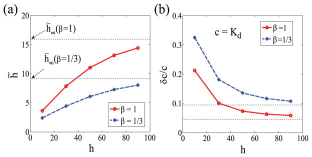
(Color online) (a) h̃ versus h for two different values of β: β = 1 (solid red line) and β = 1/3 (dashed blue line). (b) δc/c versus h at c = K_d for β = 1 (solid red line) and β = 1/3 (dashed blue line). The dotted lines correspond to the limit values of h̃ in (a) and δc/c in (b) under the limit h → ∞. We have used K_d = 100, τ_y = 1, τ_x = 10, and T = 100 in numerical simulations.

C. General limit to biochemical sensing

The mean input level c is encoded by the output sensory signal. By the law of large numbers, the statistic Z̄_T should converge to $\langle {\overline{Z}}_T\rangle =\stackrel{\sim }{f}(c)\approx c^{\stackrel{\sim }{h}}/(c^{\stackrel{\sim }{h}}+K_d^{\stackrel{\sim }{h}})$. Thus, a good estimator of c can be found by inverting Z̄_T = f̃(c). When the integration time T is sufficiently large, the output noise ${\sigma }_{z,T}^2$ can be small enough so that one can use the error propagation formula to examine the accuracy (δc/c) of this estimator. By further using Eq. (12), we have that

$$\frac{{\xi }_x^T\rho }{{\stackrel{\sim }{h}}^2{\sigma }_y^2}<{\left(\frac{\delta c}{c}\right)}^2=\frac{{\sigma }_{z,T}^2}{c^2}{\left[\frac{d\stackrel{\sim }{f}}{dx}(c)\right]}^{-2}<\frac{{\xi }_x^T}{{\stackrel{\sim }{h}}^2{\sigma }_y^2{N}_{\text{eff}}},$$ (21)

where ${\sigma }_y^2\approx {(c{K}_d)}^{\stackrel{\sim }{h}}/{(c^{\stackrel{\sim }{h}}+K_d^{\stackrel{\sim }{h}})}^2$. Equation (21) shows that ultrasensitivity (h̃) could help the system read out the input level. However, this effect is limited due to the constraint h̃ < h̃_∞. Interestingly, increasing the intrinsic Hill coefficient h increases the sensitivity (h̃), which tends to reduce the sensing error, but with fluctuations in the input it also increases the correlations between receptors (ρ) and hence decrease the effective number of sensors (N_eff), which tends to raise the sensing error. This tradeoff demonstrates the interplay between the sensitivity and the efficiency of sensors when the input is noisy. From numerical experiments, it is also found that the sensing error overall decreases with increasing h but saturates as h → ∞, as can be seen in Fig. 5(b).

Is there some fundamental limit to biochemical sensing? If the input is directly observable and we estimate the mean concentration from the sample X(t) over a time window T, then the total variance is ${\sigma }_{x,T}^2={\sigma }_x^2{\xi }_x^T$ and the sensing limit is ${(\delta c/c)}^2={\sigma }_{x,T}^2/c^2={\xi }_x^T{({\sigma }_x/c)}^2$. If X(t) is not directly observable and the mean level c has to be inferred from some output, then the actual sensing error must be larger than the sensing limit, i.e.,

$${\left(\frac{\delta c}{c}\right)}^2>{\left(\frac{{\sigma }_x}{c}\right)}^2{\xi }_x^T=\frac{{\xi }_x^T}{\beta c}.$$ (22)

This inequality sets the lower bound for the measurement error in biological sensing systems. This lower bound is solely determined by the input properties (σ_x, c, and ${\xi }_x^T$). In fact, the general inequality Eq. (22) can easily recover the Berg-Purcell limit. When X(t) refers to the number of molecules diffusing (with diffusion coefficient D) in an open volume of radius R, the input correlation time is [4]: ${\tau }_x=\frac{2}{5}{R}^2/D$, which is the typical time for molecules within the volume to be renewed by diffusion. For T ≫ τ_x, we also have ${\xi }_x^T\approx 2{\tau }_x/T$. The number of molecules in this volume is a Poisson random variable, satisfying (σ_x/c)² = 1/c where c ≡ 4π R³c̄/3 is the average number of molecules in the volume with c̄ denoting the mean concentration. Plugging all these results into Eq. (22) leads to the following inequality,

$${\left(\frac{\delta c}{c}\right)}^2>\frac{3}{4\pi R^3\overline{c}}·\frac{4R^2}{5DT}=\frac{3}{5\pi DR\overline{c}T},$$ (23)

which recovers the Berg-Purcell limit for the perfect monitor that counts the number of molecules inside itself [4]. According to Eq. (23), no matter how many or how sensitive receptors are used, the sensing error is always bounded from below by the counting noise. In fact, one can view Eq. (22) as a generalized form of the Berg-Purcell limit, as it can be applied to both Poisson and non-Poisson process.

Unlike the perfect monitor, an ultrasensitive sensor usually responds only to a narrow range of the input signal. Such sensors are able to provide accurate measurements near K_d, but become insensitive to the stimuli away from K_d. The Berg-Purcell limit does not capture such locally sensitive property, whereas our Eq. (21) does. One can obtain valuable insights by considering the extreme scenario where each sensor behaves as an indicator function Eq. (16). In this limit, we have ρ → 1, N_eff → 1, and h̃ → h̃_∞ such that Eq. (21) becomes

$${\left(\frac{\delta c}{c}\right)}^2=\frac{{\xi }_x^T}{{\stackrel{\sim }{h}}_{\infty }^2{\sigma }_{\infty }^2},$$ (24)

where ${\sigma }_{\infty }^2=\mathrm{\Gamma }(\beta c,\beta K_d)[1-\mathrm{\Gamma }(\beta c,\beta K_d)]$. For βc ≫ 1, we have ${\sigma }_{\infty }^2\approx \frac{1}{4}$ at c = K_d.

Comparing Eq. (24) with Eq. (22), one can see that if h̃_∞ were larger than $2\sqrt{\beta K_d}$, then the sensing limit given by Eq. (24) would be able to beat the fundamental limit Eq. (22) at c = K_d. However, using Eq. (19), one can verify that the inequality ${\stackrel{\sim }{h}}_{\infty }<2\sqrt{\beta K_d}$ always holds for βK_d > 1. By Eq. (20), we have that

$$\frac{2\sqrt{\beta K_d}}{{\stackrel{\sim }{h}}_{\infty }}\approx \sqrt{\frac{\pi }{2}}\approx \mathrm{1.2533.}$$ (25)

In other words, the sensing error (δc/c) by an indicator sensor near K_d is roughly 25% higher than the sensing limit of a perfect monitor. This can be understood as the information gained by an infinitely sensitive receptor (h → ∞) is still less than the information collected by the perfect monitor, which records everything.

The above arguments lead to a new sensing limit near K_d for ultrasensitive systems:

$${\left(\frac{\delta c}{c}\right)}^2>\frac{{\xi }_x^T}{{\stackrel{\sim }{h}}_{\infty }^2{\sigma }_{\infty }^2}\approx \frac{\pi {\xi }_x^T}{8\beta K_d\mathrm{\Gamma }(\beta c,\beta K_d)[1-\mathrm{\Gamma }(\beta c,\beta K_d)]}.$$ (26)

Figure 6 gives a numerical comparison of the lower bound of δc/c in Eq. (26) to that in Eq. (22). One can see that our newly derived sensing limit (dashed red line) is strictly larger than the Berg-Purcell limit (solid blue line). Interestingly, the presence of input noise helps increase the dynamic range of sensing: without the input noise, the ultrasensitive receptor would be very precise at c = K_d, but almost useless elsewhere; the presence of noise effectively increases the accuracy of signaling in the neighborhood of K_d. We also plot in Fig. 6 the upper bound (dotted green line) of δc/c given by Eq. (21) for a single sensor (N = 1) with the apparent Hill coefficient h̃. The key implication of the above theoretical arguments is that, for a sensor with known K_d and the apparent sensitivity h̃, its accuracy of biochemical measurements near K_d should be bounded as follows:

$$\frac{\sqrt{{\xi }_x^T}}{{\stackrel{\sim }{h}}_{\infty }{\sigma }_{\infty }}<\frac{\delta c}{c}<\frac{\sqrt{{\xi }_x^T}}{\stackrel{\sim }{h}{\sigma }_y}.$$ (27)

FIG. 6.

(Color online) A numerical comparison between the lower bound (solid blue line) in Eq. (22) and the lower bound (dashed red line) in Eq. (26). The dotted green line corresponds to the upper bound of δc/c in Eq. (21) for a single sensor (N = 1) with h̃ = 10. The black symbols represent the Monte Carlo simulation results of δc/c by a sensor with the apparent sensitivity h̃ ≈ 10 under the Poisson noise (i.e., β = 1) at different mean concentration levels. The sensing error δc/c was calculated using the error propagation formula in Eq. (21). These black symbols fall between the bounds as indicated by Eq. (27). Other parameters used here include K_d = 100, τ_y = 1, τ_x = 10, and T = 100.

The above simple inequality has been tested by numerical simulations (black symbols in Fig. 6).

IV. CONCLUSION

In conclusion, we have presented results, both analytical and numerical, for biochemical sensing in ultrasensitive systems. First, we demonstrate that biochemical noise does not accumulate additively but is largely limited by the noise-induced correlated property of ultrasensitive sensors. This contrasts with previous belief from the linear-noise approximation, which tends to exaggerate the impact of the input noise. Second, we show that the input noise also constrains the apparent sensitivity of the system. Thus, although ultrasensitivity is able to improve the sensing accuracy, it cannot beat the physical limit set by the molecular counting noise. Finally, our analysis leads to a sensing limit for ultrasensitive systems, which is more appropriate for ultrasensitive signaling systems. In sum, the results we present in this paper provide insights about the interplay between noise and ultrasensitivity in biochemical signal detection.

References

- 1.Cluzel P, Surette M, Leibler S. Science. 2000;287:1652. doi: 10.1126/science.287.5458.1652. [DOI] [PubMed] [Google Scholar]
- 2.Huang CY, Ferrell JE. Proc Natl Acad Sci USA. 1996;93:10078. doi: 10.1073/pnas.93.19.10078. [DOI] [PMC free article] [PubMed] [Google Scholar]
- 3.Ferrell JE, Machleder EM. Science. 1998;280:895. doi: 10.1126/science.280.5365.895. [DOI] [PubMed] [Google Scholar]
- 4.Berg HC, Purcell EM. Biophys J. 1977;20:193. doi: 10.1016/S0006-3495(77)85544-6. [DOI] [PMC free article] [PubMed] [Google Scholar]
- 5.Bialek W, Setayeshgar S. Proc Natl Acad Sci USA. 2005;102:10040. doi: 10.1073/pnas.0504321102. [DOI] [PMC free article] [PubMed] [Google Scholar]
- 6.Bialek W, Setayeshgar S. Phys Rev Lett. 2008;100:258101. doi: 10.1103/PhysRevLett.100.258101. [DOI] [PubMed] [Google Scholar]
- 7.Wang K, Rappel W-J, Kerr R, Levine H. Phys Rev E. 2007;75:061905. doi: 10.1103/PhysRevE.75.061905. [DOI] [PubMed] [Google Scholar]
- 8.Rappel W-J, Levine H. Phys Rev Lett. 2008;100:228101. doi: 10.1103/PhysRevLett.100.228101. [DOI] [PMC free article] [PubMed] [Google Scholar]
- 9.Endres RG, Wingreen NS. Proc Natl Acad Sci USA. 2008;105:15749. doi: 10.1073/pnas.0804688105. [DOI] [PMC free article] [PubMed] [Google Scholar]
- 10.Hu B, Chen W, Rappel W-J, Levine H. Phys Rev Lett. 2010;105:048104. doi: 10.1103/PhysRevLett.105.048104. [DOI] [PMC free article] [PubMed] [Google Scholar]
- 11.Hu B, Chen W, Rappel W-J, Levine H. Phys Rev E. 2011;83:021917. doi: 10.1103/PhysRevE.83.021917. [DOI] [PMC free article] [PubMed] [Google Scholar]
- 12.Mora T, Wingreen NS. Phys Rev Lett. 2010;104:248101. doi: 10.1103/PhysRevLett.104.248101. [DOI] [PubMed] [Google Scholar]
- 13.Skoge M, Meir Y, Wingreen NS. Phys Rev Lett. 2011;107:178101. doi: 10.1103/PhysRevLett.107.178101. [DOI] [PubMed] [Google Scholar]
- 14.Endres RG, Wingreen NS. Phys Rev Lett. 2009;103:158101. doi: 10.1103/PhysRevLett.103.158101. [DOI] [PubMed] [Google Scholar]
- 15.Govern CC, ten Wolde PR. Phys Rev Lett. 2012;109:218103. doi: 10.1103/PhysRevLett.109.218103. [DOI] [PubMed] [Google Scholar]
- 16.Kaizu K, de Ronde W, Paijmans J, Takahashi K, Tostevin F, ten Wolde PR. Biophys J. 2014;106:976. doi: 10.1016/j.bpj.2013.12.030. [DOI] [PMC free article] [PubMed] [Google Scholar]
- 17.Shibata T, Fujimoto K. Proc Natl Acad Sci USA. 2005;102:331. doi: 10.1073/pnas.0403350102. [DOI] [PMC free article] [PubMed] [Google Scholar]
- 18.Tanase-Nicola S, Warren PB, ten Wolde PR. Phys Rev Lett. 2006;97:068102. doi: 10.1103/PhysRevLett.97.068102. [DOI] [PubMed] [Google Scholar]
- 19.Lu T, Ferry M, Weiss R, Hasty J. Phys Biol. 2008;5:036006. doi: 10.1088/1478-3975/5/3/036006. [DOI] [PubMed] [Google Scholar]
- 20.Paulsson J. Nature (London) 2004;427:415. doi: 10.1038/nature02257. [DOI] [PubMed] [Google Scholar]
- 21.Hu B, Kessler DA, Rappel W-J, Levine H. Phys Rev E. 2012;86:061910. doi: 10.1103/PhysRevE.86.061910. [DOI] [PMC free article] [PubMed] [Google Scholar]
- 22.Park H, Oikonomou P, Guet CC, Cluzel P. Biophys J. 2011;101:2336. doi: 10.1016/j.bpj.2011.09.040. [DOI] [PMC free article] [PubMed] [Google Scholar]
- 23.Hu B, Tu Y. Phys Rev Lett. 2013;110:158703. doi: 10.1103/PhysRevLett.110.158703. [DOI] [PMC free article] [PubMed] [Google Scholar]
- 24.Hu B, Kessler DA, Rappel WJ, Levine H. Phys Rev Lett. 2011;107:148101. doi: 10.1103/PhysRevLett.107.148101. [DOI] [PMC free article] [PubMed] [Google Scholar]