Synchrotron-based small-angle X-ray scattering (SAXS) of proteins in solution

Summary

With recent advances in data analysis algorithms, X-ray detectors, and synchrotron sources, small-angle X-ray scattering (SAXS) has become much more accessible to the structural biology community than ever before. Although limited to ~10 Å resolution, SAXS can provide a wealth of structural information on biomolecules in solution and is compatible with a wide range of experimental conditions. SAXS is thus an attractive alternative when crystallography is not possible. Moreover, advanced usage of SAXS can provide unique insight into biomolecular behavior that can only be observed in solution, such as large conformational changes and transient protein-protein interactions. Unlike crystal diffraction data, however, solution scattering data are subtle in appearance, highly sensitive to sample quality and experimental errors, and easily misinterpreted. In addition, synchrotron beamlines that are dedicated to SAXS are often unfamiliar to the non-specialist. Here, we present a series of procedures that can be used for SAXS data collection and basic cross-checks designed to detect and avoid aggregation, concentration effects, radiation damage, buffer mismatch, and other common problems. The protein, human serum albumin (HSA), serves as a convenient and easily replicated example of just how subtle these problems can sometimes be, but also of how proper technique can yield pristine data even in problematic cases. Because typical data collection times at a synchrotron are only one to several days, we recommend that the sample purity, homogeneity, and solubility be extensively optimized prior to the experiment.

INTRODUCTION

The recent popularity of solution small-angle X-ray scattering (SAXS) in structural investigations of proteins and other biomolecules has been motivated by algorithmic advances, availability of synchrotron radiation and commercial lab instruments, and the changing needs of structural biologists¹. While crystallography has for many years been, and still is, the primary choice in structural biology, the challenges of crystallizing increasingly complex biomolecules have necessitated new experimental approaches. At the same time, many structural studies require insight into conformational changes under physiologically relevant conditions that are difficult to access by other methods. Given these challenges, a solution-based structural technique that provides even low-resolution information is compelling. SAXS provides an excellent avenue in these cases. Although limited by resolution (~10–50 Å d-spacing), SAXS is not limited to biomolecules of a certain size, unlike electron microscopy or nuclear magnetic resonance (NMR)². SAXS can thus offer unique insight into functionally important conformational changes of various biomolecules², including complex formation³, interconversions of multiple allosteric states⁴, movements of flexible domains⁵, and macromolecular folding-unfolding^6,7. Furthermore, such changes can be studied as a function of solution condition (e.g. ligand concentration, temperature, pressure) or even time. The versatility of SAXS makes it a powerful complementary technique even when high-resolution information is available from other methods⁸.

Despite its promise, SAXS remains a technique with a steep learning curve. The goal of this protocol is to guide non-specialists with a general approach to avoid common problems in SAXS data collection and analysis. To help familiarize the reader with SAXS data, we provide example data (Supplementary Data 1) that are discussed in detail in the Anticipated Results section. In addition, to familiarize the reader with data processing prior to a SAXS experiment, we provide notes on how to perform key steps in the user-friendly open-source program RAW⁹, for which detailed video tutorials are available online (http://sourceforge.net/projects/bioxtasraw/). We note that the exact data collection procedure (e.g. exposure times, number of exposures, averaging vs. summing of exposures, degree of automation) will depend on the sample and beamline. We describe the procedure for performing SAXS manually, which we believe represents the basic form of the technique and illustrates fundamental concepts that are common to all SAXS experiments. The general workflow and the troubleshooting guide presented here can be easily adapted to beamlines outfitted with automation or other instrumentation. Likewise, although the protocol introduced here is focused on synchrotron-based SAXS of proteins, it can be modified for use with commercial lab instruments or other soluble biomolecules, such as nucleic acids¹⁰. The reader is referred to the many excellent reviews for extended discussions of SAXS theory, data collection and analysis, and applications of the technique^2,8,11–14.

Interpretation of SAXS Data

As in X-ray crystallography, SAXS derives structural information from the interaction of X-rays with the three-dimensional distribution of electrons in a sample¹⁴. In a typical SAXS setup, a collimated, monochromatic X-ray beam is incident on the sample and scatters onto a 2D detector, giving rise to a diffuse pattern (Fig. 1). Data collection requires two measurements: one of the protein solution and one of the background solution (usually, a buffer). Because proteins in solution are randomly oriented, the scattering pattern represents an average of the scattering from all possible orientations. Hence, the scattering intensity recorded on the 2D detector will not depend on the direction of the scattering vector, but only on its magnitude, q = (4π sinθ)/λ, where 2θ is defined as the scattering angle, and λ is the wavelength of the incoming X-ray beam. The 2D images can thus be integrated about the beam center to produce 1D curves of scattering intensity I vs. q, called scattering profiles, where q is typically given in units of inverse angstroms or inverse nanometer. The scattering contribution of the protein on its own is then produced by subtracting the buffer scattering profile from the protein-solution scattering profile. This background-subtracted profile is the starting point for the analysis of solution SAXS data. A wealth of structural information can be gained from such profiles, including radius of gyration (R_g), molecular mass, foldedness and flexibility, overall 3D shape, polydispersity, and maximum intraparticle distance (D_max)^2,8,14.

Figure 1. A basic SAXS setup.

A collimated, monochromatic X-ray beam incident on the sample generates scattered X-rays, which are imaged by a detector. The transmitted beam is usually blocked by a beamstop, resulting in a shadow in the image. The scattering vector, q, describes the change in direction of the elastically scattered X-rays, and is roughly parallel to the detector face in the small-angle approximation. The images are integrated to yield scattering intensity as a 1D function of q. The scattering intensity can also be expressed as a function of s = q/2π, which is equivalent to “resolution” or d-spacing in crystallography. Because q and s are often used interchangeably in the literature, the exact usage should be explicitly defined in any publication with SAXS data.

Compared with crystal diffraction data, however, SAXS data are relatively featureless and highly sensitive to experimental technique and sample quality. Common problems such as non-specific protein aggregation, polydispersity, and poor background subtractions can severely limit the interpretability of data. To minimize the chances of buffer mismatch between the protein solution and the background solution, rigorous buffer exchange should be performed. The sample purity, stability, and conformational heterogeneity should also be characterized by other techniques (e.g. SDS-PAGE, chromatography, dynamic light scattering, multiangle light scattering, and analytical ultracentrifugation) prior to performing SAXS. Caution must also be exercised in the interpretation of data. In particular, it is important to recognize that structural parameters (such as R_g, mass, and D_max) and 3D envelopes obtained by ab initio shape reconstruction methods do not correspond to specific structural states unless the sample is monodisperse to begin with. It is also noted that the value of D_max is inferred by solving the inverse Fourier transform of the scattering profile with D_max as an adjustable parameter^14,15 and is hence, sensitive to sample quality⁸ and difficult to estimate with accuracy.

Despite the challenges in data interpretation, a major strength of SAXS is that there are multiple, independent ways to arrive at the same conclusion. For example, both R_g and mass information can be derived by Guinier or pair-distance distribution analysis (as later discussed in the Procedures). In addition, several software packages exist for the analysis of the integrated scattering profiles^9,16–18, including the widely used ATSAS package, which contains tools for 3D shape reconstructions, protein flexibility analysis, analysis of mixtures of oligomeric species, and the calculation of SAXS profiles from crystal structures. Thus, confidence in data interpretation can be gained by demonstrating consistency in multiple lines of analysis.

Experimental Variables

Sample cells for SAXS typically have path lengths of 1–3 mm requiring sample volumes on the order of 10–40 μL. Depending on the beamline, samples may be loaded manually using pipettes or automatically through robotics or microfluidics^19–24. The protein concentration (in mg/mL) needed for a given signal-to-noise ratio is inversely proportional to molecular mass. Thus, while a 14-kDa protein might require 2.5 mg/ml to give a useful signal, a 66-kDa protein would require only about 0.5 mg/mL. However, SAXS is a technique that is sensitive to solution non-ideality. Interference of X-rays scattered from particles interacting in solution can distort the scattering profile, particularly at low q. Because inter-particle interactions are concentration-dependent, measurements must be made at multiple protein concentrations for every protein of interest. Concentration effects can be subtle and failure to examine these effects can lead to incorrect estimation of the structural parameters. Other techniques that are sensitive to solution non-ideality, such as analytical ultracentrifugation, can aid in optimizing solution conditions prior to a SAXS experiment.

The optimal exposure time ranges from less than a second to a couple of minutes, depending on the available X-ray intensity and the sample’s susceptibility to the X-rays²⁵. The determination of the optimal exposure time generally entails collecting multiple, short exposures per sample and then identifying the accumulated exposure at which radiation damage begins to appear in the scattering profiles (as later discussed in the Procedures). Increasing exposure times can increase the signal-to-noise ratio but will also increase the risk of radiation damage. Some beamlines offer a flow cell with constant movement of the sample to reduce damage during exposure. Due to the physics of pressure-driven flow inside the flow cell, however, the flow velocity at the cell walls will be theoretically zero. Thus, even with constant flow, build up of damaged protein is inevitable, and the cell should be cleaned thoroughly between samples. Radiation damage will most often present itself as aggregation, which can severely limit the interpretability of data.

Preparing for Data Collection

Connecting with a Beamline

Readers can locate a convenient facility by visiting the lightsources.org website (http://www.lightsources.org/). Most synchrotron sources worldwide provide beamtime for biological SAXS via a rapid-access proposal mechanism. Potential users should consult beamline personnel to discuss the feasibility of their project, training options, and beamline-specific procedures. Many synchrotrons offer annual workshops on biological SAXS. In addition, major laboratory X-ray hardware companies offer home-source biological SAXS instrumentation that is becoming increasingly common at academic institutions.

Beamline Settings

Generally, beamline personnel will perform the setup and calibration of the beamline and provide beamline settings needed for processing raw detector files. Although it is recommended that users process data on-site at the time of collection, it is occasionally necessary to re-process data at home. Calibration steps are thus described in the Procedures (steps 12–17) to guide the user in generating beamline settings from calibration files. Users should obtain copies of these files and other necessary information needed to perform these steps from beamline personnel.

Transport of Samples

It is always advisable to prepare samples as immediately before data collection as possible. Samples that can remain monodisperse at 4 °C for periods of days to weeks should be shipped unfrozen on ice packs. Freezing can effectively arrest degradation and even time-dependent aggregation, but samples vary in their tolerance toward freezing, so care should be taken. Even when shipping frozen samples (on dry ice or in liquid nitrogen), it is advisable to reserve some unfrozen sample for comparison. Cryoprotectants are only acceptable in low concentrations (see Buffer Requirements) though on-site buffer exchange and even size exclusion chromatography are options at many beamlines.

Experimental Design

As described above, it is important to examine concentration effects for every protein of interest. An overview of preparing a concentration series is described in the Supplementary Figure 1. Another useful type of experiment is a titration, where the protein concentration is fixed and another ingredient is present at various concentrations. Such an experiment is useful for optimizing the solution condition. For example, if inter-particle repulsion is observed at a protein concentration of interest (as discussed in the Procedures and Troubleshooting), concentrated salt solutions may be used to determine an optimal ionic strength. Titration experiments are also useful for characterizing conformational changes caused by a small-molecule ligand⁴ or another protein³. Note that if a small-molecule ingredient is added to the protein solution, it must also added to the buffer solution. As discussed in the Procedures, the background buffer is best matched by performing a buffer exchange of the protein solution. However, if buffer exchange is not possible, accurate pipetting is essential.

MATERIALS

REAGENTS

• Purified protein solution

• Buffer ingredients

• Protein standards (optional)

• Small-molecule additives (optional)

• Cleaning solutions (optional)

• Liquid nitrogen (optional)

EQUIPMENT

• SAXS beamline at a synchrotron X-ray facility

• Tabletop centrifuge (one that can operate at 4 °C is desirable)

• Filters for large volumes (e.g. Nalgene, Rapid-Flow Bottle Top Filters)

• Centrifugal filters for small volumes (e.g. Corning, Costar Spin-X)

• Dialysis membranes with appropriate molecular weight cutoff

• Equipment for size-exclusion chromatography

• Disposable desalting column (e.g. GE Healthcare, PD-10)

• Centrifugal concentrator with appropriate molecular weight cutoff

• Standard microcentrifuge tubes, 1.5 ml

• UV-Vis spectrophotometer (e.g. Thermo Scientific, NanoDrop)

• A spreadsheet or graphing program

• 2D data reduction software (e.g. the open-source software RAW, available at http://sourceforge.net/projects/bioxtasraw/)

• Data analysis software (ATSAS, available at http://www.embl-hamburg.de/biosaxs/software.html)

REAGENT SETUP

Buffer Requirements

SAXS is compatible with many common biological buffers and solution conditions. Note, however, that highly electron-dense buffers (e.g. having >15% glycerol or excess metallocofactors) can lead to poor scattering contrast between the protein and background. In general, the buffer should be as dilute as possible, while having sufficient buffering strength and containing all ingredients at levels necessary for protein stability, homogeneity, and activity. Note that if the protein is highly charged at the buffer pH, the addition of salt is likely needed to reduce inter-particle effects on the scattering. Addition of glycerol, ethylene glycol, or sucrose at low concentrations (~1% w/w) to the buffer has been shown to reduce radiation damage²⁶. Common reducing agents such as DTT and TCEP are thought to provide similar protection.

Protein Requirements

SAXS is extremely sensitive to sample quality. Prior to visiting a synchrotron, the protein homogeneity should be characterized under conditions that will be used for SAXS experiments by other techniques (e.g. SDS-PAGE, size exclusion chromatography, analytical ultracentrifugation, dynamic light scattering, multiangle light scattering). By our estimates, the purity should be at least 95% by SDS-PAGE (as in crystallography). Note that because scattering signal is a function of molecular mass, even a small population of aggregates, high-order oligomers, or large impurities can significantly alter SAXS data. To reduce the chances of aggregation, it is generally recommended that samples be prepared as close to the time of use as practically possible. Samples that have been stored for significant periods of time should be subjected to size exclusion chromatography prior to use.

Protein Standards

Proteins that have been previously characterized by SAXS are useful for molecular weight determination and for evaluating the beamline setup. Beamline personnel may provide protein standards, or users can prepare their own^27,28. It is strongly advisable that protein standards be prepared fresh before use. Examples include 4.0 mg/mL hen egg white lysozyme (EMD Millipore, 5950-OP; 14.3 kDa, R_g = 14.3 ± 0.4 Å) in 40 mM sodium acetate pH 4.0, 50 mM NaCl, 1% v/v glycerol and 0.3 mg/mL glucose isomerase (Hampton Research, HR7-100; 173 kDa, R_g = 32.5 ± 0.7 Å) in 10 mM HEPES pH 7.0, 1 mM MgCl₂^28,29. Note that some proteins, such as bovine serum albumin (BSA) and human serum albumin (HSA), are prone to oligomerization and hence are not recommended as SAXS standards.

Cleaning solutions

In order to properly subtract the contributions of the sample cell to the background scattering, protein and buffer exposures should be collected using the same cell. In between different samples, the cell must be cleaned and dried. Suitable cleaning solutions include deionized water, detergent (e.g. 2% Hellmanex), bleach, and ethanol. If cleaning solutions are not provided by the beamline, consult with beamline personnel about solutions that are compatible with the sample cell.

EQUIPMENT SETUP

Beamline Setup

The typical user does not need to be directly involved in the setup of a SAXS beamline. However, prior to a synchrotron visit, the user should discuss specific needs (e.g. resolution limit, light sensitivity, oxygen sensitivity, temperature settings, detectors) with beamline personnel. Check with beamline personnel about the availability of wet lab tools, such as pipettes, disposables, tube racks, centrifuges, refrigerators, freezers, chromatography equipment, spectrophotometers, and deionized water.

Software Requirements and Setup

Software is needed for reading, displaying, integrating, and correcting detector-specific scattering images. The integrated data must also be normalized by the X-ray dose (typically measured by a PiN-diode beamstop). Unlike laboratory X-ray sources, which can be quite stable, synchrotron intensity can fluctuate and even decay over time, necessitating careful matching of actual doses. In addition to these minimum requirements, software is needed to subtract and average multiple 1D curves and perform linear fits. Suitable software may be available at the beamline. Alternatively, readers may use RAW⁹, following detailed installation and configuration instructions at http://sourceforge.net/projects/bioxtasraw/.

PROCEDURE

Preparing samples for a synchrotron trip. (Timing 1–2 d)

• 1Prepare a concentrated stock buffer solution (e.g. “10X buffer”, a stock solution at 10-fold the working concentration of the buffer) and filter sterilize with a 0.2–0.45 μm pore size membrane. Do not add ingredients that can degrade over time (e.g. reductants that may oxidize or nucleotides that can hydrolyze).
• 2Using the concentrated stock buffer solution from step 1, prepare a large volume of buffer at the working concentration, adding additional ingredients that are necessary for protein stability (but were not included in step 1), and filter. Store the remaining concentrated stock buffer solution appropriately.
• 3Using freshly diluted buffer from step 2, perform a buffer exchange of the protein solution. If the buffer components and protein are stable overnight, dialysis is an appropriate method. Alternative methods include desalting and size exclusion chromatography. CRITICAL STEP: The interpretability of SAXS data is critically dependent on the quality of the background subtraction, which requires an exact buffer background match.
• 4Save at least 50 mL (or the minimum volume recommended by beamline personnel) of the final dialysate or elution buffer from step 3. This buffer will be used for background measurements, dilutions, and sample cell cleaning at the synchrotron. In cases of size exclusion, the original reservoir buffer or the buffer from a well-equilibrated column is recommended.
• 5Concentrate the protein solution. As discussed above, typical concentrations for SAXS are in the 1–10 mg/mL range, although the minimum concentration required for sufficient scattering signal is inversely proportional to the molecular mass. Consult with beamline personnel as needed.
• 6Check the final protein concentration as accurately as possible. Errors in concentration can be a major source of error in molecular weight estimation. While no method is universally applicable, UV absorption at 280 nm (A₂₈₀ method) is widely used (when applicable) to quantify protein concentration and is accurate to approximately 10%. Potential lack of aromatic residues, the presence of interfering additives or ligands, and inaccuracies in computed extinction coefficients are complicating factors. While protein concentration is often reported in mg/mL in the SAXS literature, it is also useful to report molar concentrations if comparisons with the biochemistry literature are important.
• 7If the proteins must be frozen for storage, aliquot the protein solution from step 5 into small volumes such that they can be thawed as needed. Avoid the introduction of air bubbles and centrifuge the solutions prior to flash-freezing in liquid nitrogen.

  <PAUSE POINT> Store the frozen aliquots in liquid nitrogen or a −80°C freezer until shipping.

• 8Use the buffer from step 4 to prepare concentrated solutions of any small-molecule additives that will be later added to protein samples (e.g. ligands, salts, reductants). Concentrated salt solutions are useful for titrations if the protein has not been previously characterized by SAXS, and the optimal ionic strength is not known. If the additive is not soluble in buffer at high concentrations, dissolve in deionized water.
• 9Aliquot the additive solutions from step 8 and buffer from step 4. Store appropriately. Freeze if there are components that can degrade (e.g. oxidize, hydrolyze).

  <PAUSE POINT> Store the frozen aliquots in liquid nitrogen or a −80 °C freezer until shipping.

• 10Transport or ship samples to the synchrotron with appropriate packaging (e.g. with ice, dry ice, or liquid nitrogen). Items to include are: protein stock solutions (from step 5 or step 7, if frozen), matched buffer solutions (from step 9), additive solutions (from step 9), and 5–10 mL of concentrated stock buffer solution buffer (from step 1).
• 11Upon arrival at the synchrotron, store samples at an appropriate temperature (e.g. in a cold room, freezer, or dewar containing liquid nitrogen). Note that for samples transported on dry ice, accumulated CO₂ gas must be allowed to diffuse out from sample containers³⁰.

Preparing for data collection. (Timing 1 h)

<CRITICAL> Steps 12–17 are generally performed by beamline personnel or with the help of personnel.

• 12Configure the data reduction program to read and display the images generated by the detector.
• 13Take X-ray exposures with an empty sample cell at several exposure times. Open the images in a data reduction program and visually check that they are absent of unusual background scattering or diffuse shadows. Make note of all sharp shadows (including that of the beamstop) and pixels with unusually high (saturated) or low (dead) intensity readings.
• 14Create an integration mask in the data reduction program by outlining regions in the images that should not be included in integration (e.g. shadows and dead pixels from step 13). In RAW, masks are built by selecting mask shapes and dragging them onto the image. Right-clicking a mask and selecting “inverted mask” will mask out everything but the selected mask.
• 15Take exposures with a periodic calibrant (e.g. silver behenate powder) in the sample cell. These calibrants should be provided by beamline personnel.
• 16Determine the coordinates of the beam center and the sample-to-detector distance in the program using the lattice constant of the calibrant and the positions of the diffraction rings. Some beamlines may directly image the position of the beam center by attenuation or a semitransparent beamstop. Check that the calculated distance agrees with a physical measurement of this distance (e.g. using a tape measure). In RAW, automated calibration is initiated by opening the Centering/Calibration panel, clicking the “Start” button under Automatic Centering, and clicking on 3 or more points just outside of the innermost diffraction ring.
• 17Configure the data reduction program to convert images into 1D transmission-normalized scattering profiles (I vs q). In RAW, image integration is automatically performed as the images are generated.
• 18Document the X-ray energy, sample-to-detector distance, beam size, flux at the sample, a description of the beamline (e.g. the sample cell and detector), and other information relevant for publication¹². With the help of beamline personnel, determine how filenames of detector images and other files necessary for data processing are produced. Prepare to create a detailed log of samples and corresponding filenames when collecting data. Several hundred exposures can be produced in a single visit, and good record keeping is critical. If possible, choose a descriptive naming scheme that provides additional documentation.
• 19Plan experiments and sample recipes (Supplemental Figure 1). Start with a protein standard at a known concentration before performing experiments with the protein of interest. Consult with beamline personnel to determine sample volumes and exposure times.

  PAUSE POINT: Begin experiments when ready.

General steps for collection of a single data set. (Timing 15–30 min)

• 20Thaw any frozen stock solutions needed for the experiment. CRITICAL STEP: Do not vortex or shake vigorously as aggregates may form. Avoid repeated freeze/thaw cycles as aggregates may form.
• 21Using proper pipetting techniques, prepare a protein sample at a particular concentration and a matching buffer solution, which contains all ingredients except the protein. Keep samples at a suitable temperature (e.g. on ice). CRITICAL STEP: It is essential that any ingredients added to the protein solution be also added to the buffer solution. If any additive stock solutions were made in water (in step 8), use the concentrated stock buffer solution to compensate for the dilution of the buffer. At all times, buffer composition must match what is found in the sample solution as closely as possible (to better than 1% accuracy). Generally, it is not advisable to depend upon pipetting accuracy to make up matching buffer, but rather to exchange buffer as described in step 3.
• 22Load the buffer solution prepared in step 21 into a clean, dry sample cell without introducing air bubbles. Loading and emptying a sample cell may be performed by manual pipetting or by an automated system, depending on the beamline. CRITICAL STEP: To avoid introducing air bubbles when pipetting, dispense the liquid slowly and avoid depressing the plunger beyond the first stop.
• 23Take multiple short exposures and look for any unusual scattering in the detector images as they are generated. Note that the low readout noise of photon-counting detectors allows for large numbers of exposures to be collected and merged by averaging or summing. Integrating detectors (such as conventional CCD cameras), however, place limits on the number of frames that can be merged due to accumulation of readout noise. Consult with beamline personnel to determine how many exposures are recommended.
• 24Plot the buffer scattering profiles in the data reduction program and check that most, if not all, of the buffer profiles are superimposable to within the experimental noise level. In some automated systems, a χ-square statistic is used as a criterion for rejection.

  ? TROUBLESHOOTING

• 25Average the buffer profiles that are superimposable in the data reduction program. Check that the average curve is centered among the individual profiles. To average multiple curves in RAW, select the profiles in the Manipulation list using the shift or control key and then click on the “Average” button.
• 26Remove the buffer, rinse the sample cell with cleaning solutions (e.g. ethanol, water, detergent), and dry the cell. The goal of cleaning at this step is to prevent buffer residues from forming in the sample cell during the drying step. Cleaning solutions compatible with the sample cell should be provided by the beamlines.
• 27Remove air bubbles, aggregates, and other particulates from the protein solution (prepared in step 21) by filtration or centrifugation. To use a centrifugal filter, rinse the membrane as instructed by the manufacturer, then rinse with buffer and remove completely before filtering protein solution. Alternatively, centrifuge the solution (e.g. 16,000 x g at 4 °C for 10 min) and remove the supernatant.
• 28Repeat steps 22–24 with the protein solution. Check for any time-dependent changes in the shape of the curves. Overlay the individual protein-solution scattering profiles with the averaged buffer profile from step 25 and check that they do not cross over (beyond statistical fluctuations) at high q.

  ? TROUBLESHOOTING

• 29Average the protein-solution profiles that are superimposable following the same procedure used in step 25. Exclude profiles exhibiting time-dependent changes in scattering, particularly at low q. Note that while averaging improves the signal-to-noise ratio, it is not required for further data processing, and there are certain cases where not averaging may be preferred (see step 32).

  ? TROUBLESHOOTING

• 30Remove the protein sample and repeat the cleaning procedure in step 26.
• 31Repeat steps 22–26 with the buffer. Check that the buffer profiles before and after the protein exposures are superimposable.

  ? TROUBLESHOOTING

Background subtraction and initial inspection. (Timing 5 min)

• 32Subtract the averaged buffer profile (from step 25) from the averaged protein-solution profile (from step 29). To do this in RAW, mark the buffer profile by clicking on the adjacent star icon, select the protein-solution profile in the Manipulation list, and click the “Subtract” button. This averaged, subtracted scattering profile will be used for subsequent analyses. Note that emerging SAXS methods, such as in-line size exclusion chromatography²¹, may require that buffer subtraction be performed on individual exposures (generated in step 28) rather than the average (from step 29). Additionally, users may wish to monitor structural parameters for each exposure. In such cases, it is recommended that subtractions be performed with a buffer profile of a comparable or lower experimental noise level than the protein-solution profiles (e.g. the averaged buffer profile from step 25). CRITICAL STEP: Save subtracted data curves and/or obtain the necessary software settings from beamline personnel needed to repeat any data reduction at home.

  ? TROUBLESHOOTING

• 33Plot the buffer-subtracted profile as log(I) vs. q and inspect the shape. The semi-log plot of a typical, well-behaving protein will have a characteristic bell-like shape in the low-q region. Alternatively, plot the subtracted profile as log(I) vs. log(q), which should intersect the vertical axis roughly perpendicularly.

  ? TROUBLESHOOTING

Guinier analysis. (Timing 5–15 min)

• 34Plot the subtracted profile from step 32 as a Guinier curve (ln(I) vs. q²) and zoom into the low-q region (the maximum q² should be < 0.01 Å⁻² for most proteins). Check that the Guinier curve appears linear at low q with no obvious upturn or downturn. For a monodisperse solution of a protein with a well-defined size, this region should be linear¹². To examine Guinier curves in RAW, right-click on the profile in the Manipulation list, select “Guinier fit” in the popup menu, and adjust the axis ranges in the Guinier fit window that appears.

  ? TROUBLESHOOTING

• 35Perform a linear fit to the low-q region of Guinier curve. The maximum q that is generally acceptable to include in the fit is 1.3/R_g, where R_g is the radius of gyration of the protein¹². A small number of noisy data points in the beginning may be omitted from the fit, but any significant non-linear trends should be reported in publications. The slope of the line is equal to –R_g²/3, and the vertical intercept is equal to the natural log of the zero-angle scattering intensity, I(0). In RAW, adjust the maximum q in the Guinier fit window until the displayed qR_g value is 1.3 or less and the residuals of the fit (displayed in the bottom panel) are randomly distributed around zero.

  ? TROUBLESHOOTING

• 36
  Once steps 20–35 have been performed for a protein standard and the protein of interest, calculate the mass of the protein of interest with the equation²⁸:

  $${(I(0)/c\times \mathrm{mass})}_{\text{protein-of-interest}}={(I(0)/c\times \mathrm{mass})}_{\text{protein-standard}}.$$

  Use I(0) values from step 34 and c (protein concentration in mg/mL) from step 21. Alternatively, the use of a protein standard for mass determination can be avoided if I(0) is converted to an absolute scale using a water sample³¹.
• 37Document the R_g, I(0), and estimated mass.
• 38Before proceeding to the next solution condition, repeat steps 20–35 at least twice at different concentrations of the protein of interest. If performing these measurements sequentially, do a buffer measurement only once in between protein measurements. CRITICAL STEP: SAXS data are sensitive to solution non-ideality and are hence concentration-dependent, even in the absence of structural changes to the protein. Concentration effects can be identified by collecting data at multiple protein concentrations.

  PAUSE POINT: Perform the next set of experiments (repeating steps 20–38) when ready. The following data analysis steps (39–45) can be performed either sequentially or in parallel with data collection, depending on the number of users. If time is limited, these additional steps can be performed at home.

Pair-distance distribution analysis and evaluation of concentration effects. (Timing 15 min)

• 39Prepare a text file in ASCII format containing q and I values (and optionally, the standard deviation of I), delimited by a space or comma. In RAW, the scattering curve can be saved as an ASCII file by selecting subtracted curve in the Manipulation list and clicking the “Save” button.
• 40Open the ASCII file in the cross-platform version of PRIMUS¹⁷ (PRIMUS Qt) from the ATSAS package and select “Distance Distribution” from the Tools menu. The resultant window will call the program GNOM¹⁵, which generates the Fourier transform of I(q): the pair-distance distribution function, P(r), which represents a continuous r²-weighted histogram of all electron-pair distances, r, in the protein. In this process, the program will automatically optimize the q-range included in the analysis and estimate the maximum dimension of the protein, D_max. If P(r) is severely negative or highly extended at high r, the data may not be suitable for further analysis. CRITICAL STEP: This step is designed to provide an initial guess for D_max for the non-expert user, and it is generally not recommended to automate D_max estimation.

  ? TROUBLESHOOTING

• 41In the same GNOM window, release the default condition that fixes P(r) to zero at high r. If P(r) no longer converges to zero at high r, manually adjust D_max and the q-range included in the analysis (q_min to q_max) until P(r) naturally approaches zero. The q_min value can be adjusted to exclude data that exhibits inter-particle effects or noise, but it should not exceed the value set by the so-called Shannon Limit³² (q = π/D_max). The q_max value can be adjusted to avoid over-fitting low signal-to-noise data in the high q region. P(r) of high-quality data with negligible inter-particle effects will not only converge to zero at high r at a certain D_max, but will also remain converged even when D_max is further increased. The reader is referred to the literature⁸ for an excellent review of D_max estimation.

  ? TROUBLESHOOTING

• 42Save the output file from step 41. CRTICAP STEP: Note that steps 40 and 41 can also be performed using the standalone versions of DATGNOM³³ and GNOM¹⁵, respectively. In all cases, an output file will be generated with the results from the set of parameters that were tested last. The output file will also include a rating of “suspicious”,”reasonable”,”good”, or “excellent” based on the quality score known as the Total Estimate. While acceptable solutions should be rated “reasonable” or better, it is important to visually inspect the shape of P(r) and the corresponding fit to I(q).
• 43Compare the R_g and I(0) determined from P(r) (step 40 or 41) with the corresponding values determined by Guinier analysis (step 37). The values should agree within error.
• 44In a spreadsheet or graphing program, plot R_g and I(0) values determined by each method (P(r) and Guinier) at three or more protein concentrations. For each plot, the trends should appear roughly linear over a concentration range. If the trends increase significantly or nonlinearly with increased concentration, it is likely that the protein is a mixture of oligomers or is aggregated.

  ? TROUBLESHOOTING

• 45Fit a line to the plot of R_g versus concentration (for each method, P(r) and Guinier). The vertical intercept of this line is the R_g extrapolated to infinite dilution.

  PAUSE POINT: Further analyses can be performed at home. Once a reasonable P(r) has been obtained, the output file from step 42 can be used in ab initio shape reconstruction programs. It is important to note that shape reconstructions are not meaningful unless the homogeneity of the sample has been demonstrated by other methods. Note also that to perform shape reconstructions in DAMMIF or DAMMIN^34,35, the recommended limit for the maximum q in P(r) analysis is 8/R_g. Finally, estimate molecular mass with another method, if possible. Mass can be estimated without a protein standard by putting I(0) on an absolute scale³¹. Mass can also be estimated without concentration information using one of several methods based on integral invariants^14,36–38. Mass estimates should agree to within an expected error of approximately 10%.

TIMING

• Steps 1–11, Preparing samples for a synchrotron trip: 1–2 d

• Steps 12–19, Preparing for data collection, 1 h

• Steps 20–31, General steps for collection of a single data set, 15–30 min

• Steps 32–33, Background subtraction and initial inspection, 5 min

• Steps 34–38, Guinier analysis, 5–15 min

• Steps 39–45, Pair-distance distribution analysis and evaluation of concentration effects, 15 min

TROUBLESHOOTING

For troubleshooting advice refer to Table 1.

Table 1.

Troubleshooting

Step	Problem	Possible Reason	Possible Solution
24	Sequential buffer profiles do not superimpose in a time-independent manner.	Air bubbles in the beam path, sample is moving out of beam (if using flow cell), or problem with intensity normalization.	Repeat steps 22–24 with a clean and dry cell, taking care to avoid air in the beam path. If problem recurs, consult beamline personnel to check intensity normalization.
28	Buffer and protein-solution profiles do not appear to converge at high q.	Buffer mismatch.	Repeat steps 27–28 with freshly made sample. If problem recurs, make up the buffer first, and then exchange into the buffer with a desalting column.
29	Sequential protein-solution profiles do not superimpose in a time-independent manner.	Air bubbles in the beam path, sample is moving out of beam (if using flow cell), or problem with intensity normalization.	Repeat step 27–29 with a clean and dry cell using fresh sample, taking care to avoid air in the beam path. If problem recurs, consult beamline personnel to check intensity normalization.
29	Scattering signal of protein-solution profiles appears to be increasing as a function of time.	Radiation damage.	Repeat step 27–29 with a clean and dry cell using fresh sample. Use faster flow rates (when using a flow cell), shorter exposure times, or 5–10 sec pauses in between exposures to allow radiation-induced aggregates to diffuse away from the beam path. If problem recurs, consider adding or increasing the concentration of additives with protective effects against radiation damage (refer to Buffer Requirements).
31	Buffer profiles before and after protein exposures are not superimposable.	Buildup of protein residue on the walls of the sample cell, contaminants were introduced, or change in the beamline setup (e.g. vacuum leak, beam drift).	Repeat steps 20–31 with more a rigorous cleaning procedure (possibly using harsher cleaning solutions, e.g. detergent). Ask beamline personnel to check the beamline and install a fresh sample cell, if possible.
32	Buffer subtraction yields negative signal or an under-subtracted signal at high q.	Buffer mismatch, poor intensity normalization, poor cleaning of the sample cell, or a change in the beamline setup (e.g. vacuum leak, beam drift).	Perform a buffer exchange with a disposable desalting column. Repeat steps 20–31 with more a rigorous cleaning procedure (possibly using harsher cleaning solutions). Ask beamline personnel to check the beamline setup.
33	The log(I) vs log(q) plot of the background-subtracted profile shows a steep increase at low q.	Aggregation or radiation damage.	Proceed to step 34 for better diagnosis.
34	Guinier curve has an upturn at low q.	Aggregation or radiation damage.	Perform a buffer subtraction of just the first protein exposure and plot as Guinier curve. If there is no upturn, systematically determine the number of exposures that are free of radiation damage and produce a new average (step 28). If upturn is observed in the first exposure, filter or extensively centrifuge fresh sample, and repeat steps 28–29. If the pH of the buffer is close to the isoelectric point (pI) of the protein, reduce the salt concentration or change the pH away from the pI.
34	Guinier curve has a downturn at low q.	Inter-particle repulsion.	Repeat steps 27–29 at a lower protein concentration or higher salt concentration.
35	Not enough data points in the Guinier curve satisfying qRg<1.3 criterion.	Protein is too large for the current beamline setup.	Consult with beamline personnel about changing detector or beamstop position.
40	Negative P(r) at high r.	Inter-particle repulsion.	If severe, repeat steps 27–29 at a lower protein concentration or higher salt concentration.
40	Highly extended P(r) at high r.	Aggregation or oligomerization, though extended P(r) may represent true structural features.	If severe, filter or extensively centrifuge fresh sample and repeat steps 28–29. Alternatively, reduce the protein concentration or change the solution condition. If the pH of the buffer is close to the isoelectric point (pI) of the protein, reduce the salt concentration or change the pH away from the pI.
41	Slightly negative or positive P(r) at high r.	Subtle inter-particle effects or slight aggregation.	Adjust the q-range (particularly qmin).
43	Trends increase significantly or nonlinearly with increasing concentration.	Protein is a mixture of oligomers under this solution condition.	Repeat steps 27–29 at below or above transition if data on monodisperse samples are desired. Alternatively, change the solution conditions.

ANTICIPATED RESULTS

The protocols introduced here are demonstrated by data collected on human serum albumin (HSA). 1 L of buffer (50 mM HEPES pH 7.5, 100 mM NaCl) was prepared, filtered (Nalgene Rapid-Flow, 0.2 μm PES), and de-gassed. Lyophilized HSA (Sigma, A8763) was dissolved in the buffer at ~10 mg/mL and filtered (Corning Spin-X, 0.22 μm cellulose acetate). Buffer exchange was performed in two ways. In the first method, HSA was separated from small molecules (e.g. stabilizers introduced in the lyophillization process) by using a disposable desalting column (GE Healthcare, PD-10). In the second, monomeric HSA was separated from both small molecules and oligomeric forms of HSA by size exclusion chromatography (GE Healthcare, Superdex-200) (Fig. 2). The eluted proteins were concentrated using centrifugal concentrators (GE Healthcare, Vivaspin 6, 30 kDa MWCO), and the final concentration was determined from the absorption at 280 nm³⁹.

Figure 2. Size exclusion chromatogram of HSA.

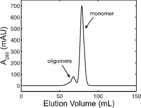
Multiple peaks are observed, indicating that the HSA solution is a monomer-oligomer mixture prior to this purification step.

Samples were loaded in an in vacuo oscillating flow cell²². Scattering images were collected on a fiber-optic-coupled CCD detector⁴⁰ and were corrected⁴¹, integrated, and normalized by the transmission intensity to generate 1D scattering profiles, I vs. q (Supplementary Data 1). Typical scattering profiles prior to buffer subtraction are shown in Fig. 3. The effect of buffer mismatch is shown in Fig. 4. Following inspection of the profiles, averaging and buffer subtraction was performed as described in the procedures.

Figure 3. Typical scattering from protein solution (red) and the corresponding buffer (gray).

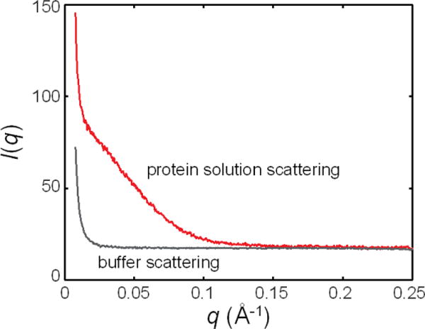
The scattering profiles are offset by a constant positive value. Note that apart from the sharp upturn at low q, the background scattering is largely featureless.

Figure 4. Examples of good and bad buffer subtractions.

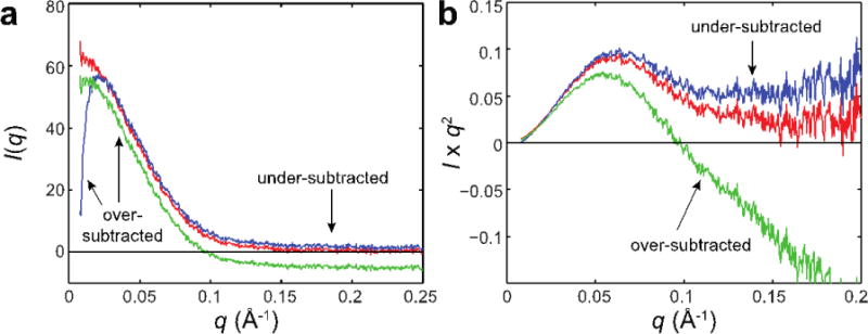
(a) Here, the scattering from HSA solution is subtracted with that of a matched buffer (red), a different buffer at another pH (blue), and a similar buffer with glycerol added (green). Note that proper subtractions should lead to positive intensity values that, for a well-folded protein, approach near zero at high q. In these examples, buffer mismatch leads to extreme over-subtraction at low q and unphysical, negative intensities or artificially high, positive intensities at high q. It is important to note, however, that distortions of the scattering profile at low q can be a real consequence of inter-particle interactions. Similarly, less compact forms of proteins will not exhibit a sharp intensity fall-off at high q. Thus, confidence in buffer subtractions is absolutely essential for proper interpretation of data. (b) The scattering behavior at high q is enhanced when plotted as Kratky curves (same colors as in (a)).

The importance of sample homogeneity is demonstrated by data collected on HSA. Although the lyophilized HSA used here is ≥99% pure in terms of protein content, HSA is known to form oligomers through inter-molecular disulfides, which must be separated by size exclusion⁴² (Fig. 2). Notably, the buffer-subtracted profiles and the corresponding Guinier curves of unpurified HSA show no obvious problems (Fig. 5a–b, red). However, subtle differences are apparent when compared with the scattering profiles of purified HSA (Fig. 5a–b, black). For a given concentration (in mg/mL), both the vertical intercept and slope of the Guinier curves are slightly greater when size exclusion is not performed (Fig. 5b), consistent with the presence of oligomers in these samples.

Figure 5. Comparison of HSA with and without the final purification step.

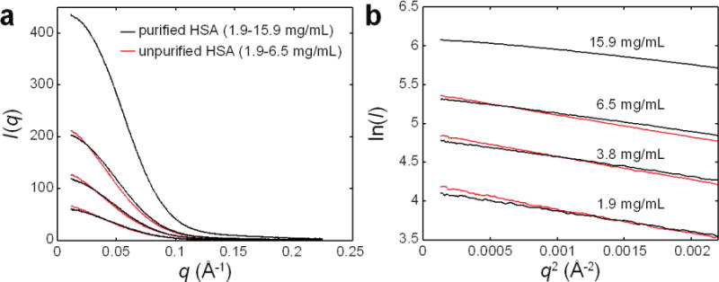
(a) The scattering profiles of unpurified HSA (red curves, from bottom to top: 1.9, 3.8, 6.5 mg/mL) and purified HSA (black curves, from bottom to top: 1.9, 3.8, 6.5, 15.4 mg/mL) show no signs of aggregation, which would appear as upturns in the lowest q portion of a profile. (b) When plotted as Guinier curves, the absence of upturns at low q is clear. In addition, the effect of the final purification step is evident: for a given concentration, the slope and vertical intercept of unpurified HSA are greater, consistent with the presence of species larger than a monomer. Finally, concentration effects can be seen, particular in the case of purified HSA. With increasing concentration, a greater downward curvature is observed at low q, consistent with inter-particle repulsion.

The importance of examining multiple protein concentrations is also demonstrated by these data. Inter-particle interactions occur over large length scales and hence distort scattering profiles in a concentration-dependent manner at low q, where Guinier analysis is performed (Fig. 6). In the case of HSA, the R_g values determined by Guinier analysis decrease roughly linearly with increasing concentration (Fig. 7a), a trend that is consistent with inter-particle repulsion arising from excluded volume effects^10,43. Linear fits to these trends yield R_g values extrapolated to infinite dilution (i.e. where inter-particle effects are minimized) of 28.7 ± 1.1 Å and 32.7 ± 4.4 Å for purified and unpurified HSA, respectively. Here, the error estimates represent the 95% confidence intervals from the fits. In the case of I(0), a linear trend is observed for samples over the 1.9–6.5 mg/mL range (Fig. 7b). The I(0) value for purified HSA at 15.9 mg/mL, however, falls short of this linear trend. Inspection of the Guinier curve for this sample shows that I(0) is underestimated because of a subtle downward curvature in the low q region due to inter-particle repulsion (Fig. 5b).

Figure 6. Example of Guinier analysis.

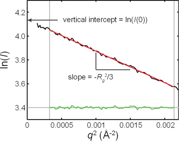
A line (red) is fitted to the low q region of a Guinier curve (black), such that maximum q to be included in the fit is 1.3/R_g or less. The linearity of the fitted region is determined by the flatness of the residuals (green). R_g is derived from the slope, and I(0) is derived from the vertical intercept.

Figure 7. Concentration effects on R_g and I(0).

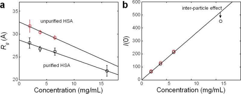
(a) For both purified (black) and unpurified (red) HSA, the R_g values from Guinier analysis show a decreasing linear trend with increasing protein concentration. The error bars represent standard deviations from linear fits to the Guinier curves in Fig. 6. This trend is caused by distortions in the scattering profiles at low q that arise from inter-particle repulsion. (b) Over the 1.9 – 6.5 mg/mL range, I(0) shows a linear relationship with protein concentration for both purified (black) and unpurified (red) HSA. Deviations from a linear trend can be indicative of inter-particle effects or changes in oligomerization state.

The effects of inter-particle interactions and polydispersity are very evident in the pair distance distribution, P(r)⁸. Because of the reciprocal relationship of r and q, inter-particle effects at low q affect the high-r portion of P(r). Aggregates or oligomers, such as those found in unpurified HSA solutions, can lead to an artificially high D_max (Fig. 8, dotted), and in the worst cases, P(r) will not converge to zero at high r. Conversely, inter-particle repulsion, such as that observed for purified HSA at 15.9 mg/mL, will lead to negative P(r) at high r (Fig. 8, blue). Dilution of HSA leads to P(r) curves that are nearly superimposable, except at high r where the curves become less negative (Fig. 8, blue to red). This trend is consistent with the reduction of inter-particle effects. At 1.9 mg/mL, these effects are negligible, resulting in a P(r) curve that tends smoothly towards zero with a well-defined D_max (Fig. 8, red). The sensitivity of P(r) to inter-particle interactions and polydispersity makes this analysis is a useful step in inspecting data quality.

Figure 8. The pair distance distribution function, P(r), is sensitive to concentration effects and sample polydispersity.

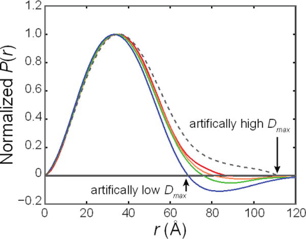
Here, PRIMUS¹⁷ was used to automatically generate the P(r) of purified HSA (solid curves, from red to blue: 1.9–15.9 mg/mL) and unpurified HSA at 1.9 mg/mL (dotted curve). Inter-particle repulsion leads to negative regions at high r, which leads to an artificially low D_max. The presence of aggregates or higher order oligomers extends P(r) at high r, leading to an artificially high D_max.

Following these analyses, ab initio shape reconstructions can be performed for data collected on homogeneous samples with negligible inter-particle effects. In the case of HSA, homogeneity is achieved with size-exclusion chromatography (Fig. 2), and inter-particle effects are minimized through serial dilutions (Figs. 7a, 8). However, dilute samples that exhibit nearly ideal solution behavior may not have sufficient signal-to-noise levels at high q needed for shape reconstructions and other types of analyses (e.g. Kratky and Porod exponent analyses). In such cases, it is possible to apply extrapolation methods that combine data collected at multiple concentrations if it can be shown that the sample does not appreciably change its conformation^17,31. This assumption is not necessarily valid in all situations. Merging or extrapolation operations should thus be performed with caution and always be reported¹².

In the case of purified HSA, the P(r) curves are largely identical at all concentrations except at high r (Fig. 8, solid), indicating that there are no appreciable conformational changes. Equivalently, the I(q) curves are also superimposable except at low q. Low q data from 1.9 mg/mL purified HSA (q range of .008 – .045 Å⁻¹) was thus merged with higher q data from 3.8 mg/mL purified HSA (q range of .035 – .22 Å⁻¹) in PRIMUS¹⁷ (Fig. 9a, gray). A smooth curve was fitted (Fig. 9a, black) to the data in GNOM¹⁵, producing a P(r) curve that converges smoothly to zero at high r. Because shape reconstructions do not yield unique solutions, ten bead models were thus reconstructed in DAMMIF³⁵ (Supplementary Video 1), aligned and averaged in DAMAVER⁴⁴ to produce a most probably model, and refined in DAMMIN³⁴ to produce the final SAXS envelope (Fig. 9b, surface). It is important to note that the solution conformation of a protein does not have to agree with the conformation observed in crystal structures. In the case of HSA, however, the final SAXS envelope of monomeric HSA (as determined by size exclusion) shows good agreement with the crystal structure of the HSA monomer⁴⁵ (Fig. 9b). Similarly, the theoretical scattering profile of this crystal structure⁴⁵ generated in CRYSOL⁴⁶ also shows good agreement to the experimental profile (Fig. 9a, magenta).

Figure 9. Comparisons to a crystal structure.

(a) Low q data from 1.9 mg/mL purified HSA was merged with higher q data from 3.8 mg/mL purified HSA (shown in gray with standard errors⁴⁷). A smooth curve was fitted (black) to the data in GNOM¹⁵ that yielded a well-behaved P(r) curve. Ten bead models were reconstructed in DAMMIF³⁵, which were aligned and averaged in DAMAVER⁴⁴ with no rejections and a normalized spatial discrepancy of 0.874 ± 0.032. The fit of a typical DAMMIF model (cyan) shows good agreement to the data as does the theoretical scattering profile of a crystal structure⁴⁵ (magenta). (b) Following averaging in DAMAVER, the “damstart” model was used for a round of refinement in DAMMIN³⁴, yielding the final SAXS envelope (gray), shown superimposed with the crystal structure⁴⁵ (magenta).

Supplementary Material

Figure S1

Supplemental Figure 1: Planning a concentration series experiment. To perform a concentration series experiment, proteins solutions must be prepared at three or more protein concentrations in the same buffer (here, represented as protein solutions #1–3). For each sample, the total volume should be equal to or greater than the minimum volume required by the sample cell. Recipes should be designed such that mixing volumes can be pipetted accurately. Multiple X-ray exposures are collected on each protein solution and matching buffer as described in the Procedures. Data are then reduced (i.e. by averaging and subtraction) in order to produce a single background-subtracted scattering profile, from which structural information can be gained. Multiple background-subtracted scattering profiles at different protein concentrations are then required to examine concentration effects and estimate structural parameters, such as R_g at infinite dilution. As many exposures are generated in a single experiment, careful and detailed documentation is indispensable.

Supplementary Data 1: Example data on HSA. The compressed archive file contains all buffer-subtracted profiles introduced in the Anticipated Results section as well as examples of unsubtracted, unaveraged profiles. Data files are in ASCII format with columns corresponding to q, I, and the standard deviation of I.

Supplementary Video 1: Representative shape reconstruction. The simulated annealing of a typical HSA bead model in DAMMIF³⁵ is shown. Note that although crystal structure is superimposed for comparison, individual reconstructions prior to averaging should not be over-interpreted.

References

- 1.Nagar B, Kuriyan J. SAXS and the working protein. Structure. 2005;13:169–170. doi: 10.1016/j.str.2005.01.001. [DOI] [PubMed] [Google Scholar]
- 2.Putnam CD, Hammel M, Hura GL, Tainer JA. X-ray solution scattering (SAXS) combined with crystallography and computation: defining accurate macromolecular structures, conformations and assemblies in solution. Q Rev Biophys. 2007;40:191–285. doi: 10.1017/S0033583507004635. [DOI] [PubMed] [Google Scholar]
- 3.Ando N, et al. Transient B(12)-Dependent Methyltransferase Complexes Revealed by Small-Angle X-ray Scattering. Journal of the American Chemical Society. 2012;134:17945–17954. doi: 10.1021/ja3055782. [DOI] [PMC free article] [PubMed] [Google Scholar]
- 4.Ando N, et al. Structural interconversions modulate activity of Escherichia coli ribonucleotide reductase. PNAS. 2011;108:21046–21051. doi: 10.1073/pnas.1112715108. [DOI] [PMC free article] [PubMed] [Google Scholar]
- 5.Rambo RP, Tainer JA. Characterizing flexible and intrinsically unstructured biological macromolecules by SAS using the Porod-Debye law. Biopolymers. 2011;95:559–571. doi: 10.1002/bip.21638. [DOI] [PMC free article] [PubMed] [Google Scholar]
- 6.Pollack L, et al. Compactness of the denatured state of a fast-folding protein measured by submillisecond small-angle x-ray scattering. Proceedings of the National Academy of Sciences of the United States of America. 1999;96:10115–10117. doi: 10.1073/pnas.96.18.10115. [DOI] [PMC free article] [PubMed] [Google Scholar]
- 7.Pollack L, et al. Time resolved collapse of a folding protein observed with small angle x-ray scattering. Physical Review Letters. 2001;86:4962–4965. doi: 10.1103/PhysRevLett.86.4962. [DOI] [PubMed] [Google Scholar]
- 8.Jacques DA, Trewhella J. Small-angle scattering for structural biology-Expanding the frontier while avoiding the pitfalls. Protein Science. 2010;19:642–657. doi: 10.1002/pro.351. [DOI] [PMC free article] [PubMed] [Google Scholar]
- 9.Nielsen SS, et al. BioXTAS RAW, a software program for high-throughput automated small-angle X-ray scattering data reduction and preliminary analysis. Journal of Applied Crystallography. 2009;42:959–964. [Google Scholar]
- 10.Pollack L. SAXS Studies of ion-nucleic acid interactions. Annu Rev Biophys. 2011;40:225–242. doi: 10.1146/annurev-biophys-042910-155349. [DOI] [PubMed] [Google Scholar]
- 11.Graewert MA, Svergun DI. Impact and progress in small and wide angle X-ray scattering (SAXS and WAXS) Current Opinion in Structural Biology. 2013:1–7. doi: 10.1016/j.sbi.2013.06.007. [DOI] [PubMed] [Google Scholar]
- 12.Jacques DA, Guss JM, Svergun DI, Trewhella J. Publication guidelines for structural modelling of small-angle scattering data from biomolecules in solution. Acta Crystallographica Section D. 2012;68:620–626. doi: 10.1107/S0907444912012073. [DOI] [PubMed] [Google Scholar]
- 13.Pérez J, Nishino Y. Advances in X-ray scattering: from solution SAXS to achievements with coherent beams. Current Opinion in Structural Biology. 2012 doi: 10.1016/j.sbi.2012.07.014. [DOI] [PubMed] [Google Scholar]
- 14.Glatter O, Kratky O. Small Angle X-ray Scattering. Academic Press; 1982. [DOI] [PubMed] [Google Scholar]
- 15.Svergun DI. Determination of the regularization parameter in indirect-transform methods using perceptual criteria. Journal of Applied Crystallography. 1992;25:495–503. [Google Scholar]
- 16.Konarev PV, Petoukhov MV, Volkov VV, Svergun DI. ATSAS 2.1, a program package for small-angle scattering data analysis. Journal of Applied Crystallography. 2006;39:277–286. doi: 10.1107/S0021889812007662. [DOI] [PMC free article] [PubMed] [Google Scholar]
- 17.Konarev PV, Volkov VV, Sokolova A, Koch MHJ, Svergun DI. PRIMUS: a Windows PC-based system for small-angle scattering data analysis. Journal of Applied Crystallography. 2003;36:1277–1282. [Google Scholar]
- 18.Schneidman-Duhovny D, Hammel M, Sali A. FoXS: A web server for rapid computation and fitting of SAXS profiles. Nucleic Acids Research. 2010;38:W540–544. doi: 10.1093/nar/gkq461. [DOI] [PMC free article] [PubMed] [Google Scholar]
- 19.Hura GL, M A, Hammel M, Rambo RP, Poole FL, II, Tsutakawa SE, Jenney FE, Jr, Classen S, Frankel KA, Hopkins RC, Yang S, Scott JW, Dillard BD, Adams MWW, Tainer JA. Robust, high-throughput solution structural analyses by small angle X-ray scattering (SAXS) Nature Methods. 2009;6:606–612. doi: 10.1038/nmeth.1353. [DOI] [PMC free article] [PubMed] [Google Scholar]
- 20.Lafleur JP, et al. Automated microfluidic sample-preparation platform for high-throughput structural investigation of proteins by small-angle X-ray scattering. Journal of Applied Crystallography. 2011;44:1090–1099. [Google Scholar]
- 21.Mathew E, Mirza A, Menhart N. Liquid-chromatography-coupled SAXS for accurate sizing of aggregating proteins. Journal of synchrotron radiation. 2004;11:314–318. doi: 10.1107/S0909049504014086. [DOI] [PubMed] [Google Scholar]
- 22.Nielsen SS, Møller M, Gillilan RE. High-throughput biological small-angle X-ray scattering with a robotically loaded capillary cell. Journal of Applied Crystallography. 2012;45:213–223. doi: 10.1107/S0021889812000957. [DOI] [PMC free article] [PubMed] [Google Scholar]
- 23.Pernot P, et al. New beamline dedicated to solution scattering from biological macromolecules at the ESRF. Journal of Physics: Conference Series. 2010;247:012009. [Google Scholar]
- 24.Round AR, et al. Automated sample-changing robot for solution scattering experiments at the EMBL Hamburg SAXS station X33. Journal of Applied Crystallography. 2008;41:913–917. doi: 10.1107/S0021889808021018. [DOI] [PMC free article] [PubMed] [Google Scholar]
- 25.Fischetti RF, et al. High-resolution wide-angle X-ray scattering of protein solutions: effect of beam dose on protein integrity. Journal of Synchrotron Radiation. 2003;10:398–404. doi: 10.1107/s0909049503016583. [DOI] [PubMed] [Google Scholar]
- 26.Kuwamoto S, Akiyama S, Fujisawa T. Radiation damage to a protein solution, detected by synchrotron X-ray small-angle scattering: dose-related considerations and suppression by cryoprotectants. Journal of synchrotron radiation. 2004;11:462–468. doi: 10.1107/S0909049504019272. [DOI] [PubMed] [Google Scholar]
- 27.Akiyama S. Quality control of protein standards for molecular mass determinations by small-angle X-ray scattering. Journal of Applied Crystallography. 2010;43:237–243. [Google Scholar]
- 28.Mylonas E, Svergun DI. Accuracy of molecular mass determination of proteins in solution by small-angle X-ray scattering. Journal of Applied Crystallography. 2007;40:s245–s249. [Google Scholar]
- 29.Kozak M. Glucose isomerase from Streptomyces rubiginosus-potential molecular weight standard for small-angle X-ray scattering. J Appl Cryst. 2005;38:555–558. [Google Scholar]
- 30.Murphy BM, et al. Protein instability following transport or storage on dry ice. Nature Methods. 2013;10:278–279. doi: 10.1038/nmeth.2409. [DOI] [PubMed] [Google Scholar]
- 31.Orthaber D, Bergmann A, Glatter O. SAXS experiments on absolute scale with Kratky systems using water as a secondary standard. Journal of Applied Crystallography. 2000;33:218–225. [Google Scholar]
- 32.Moore PB. Small-Angle Scattering. Information Content and Error Analysis. Journal of Applied Crystallography. 1980;13:168–175. [Google Scholar]
- 33.Gherardi E, et al. Structural basis of hepatocyte growth factor/scatter factor and MET signalling. Proceedings of the National Academy of Sciences of the United States of America. 2006;103:4046–4051. doi: 10.1073/pnas.0509040103. [DOI] [PMC free article] [PubMed] [Google Scholar]
- 34.Svergun DI. Restoring low resolution structure of biological macromolecules from solution scattering using simulated annealing. Biophysical Journal. 1999;76:2879–2886. doi: 10.1016/S0006-3495(99)77443-6. [DOI] [PMC free article] [PubMed] [Google Scholar]
- 35.Franke D, Svergun DI. DAMMIF, a program for rapid ab-initio shape determination in small-angle scattering. Journal of Applied Crystallography. 2009;42:342–346. doi: 10.1107/S0021889809000338. [DOI] [PMC free article] [PubMed] [Google Scholar]
- 36.Fischer H, Oliveira Neto Md, Napolitano HB, Polikarpov I, Craievich AF. Determination of the molecular weight of proteins in solution from a single small-angle X-ray scattering measurement on a relative scale. Journal of Applied Crystallography. 2009;43:101–109. [Google Scholar]
- 37.Rambo RP, Tainer JA. Accurate assessment of mass, models and resolution by small-angle scattering. Nature. 2013;496:477–481. doi: 10.1038/nature12070. [DOI] [PMC free article] [PubMed] [Google Scholar]
- 38.Petoukhov MV, et al. New developments in the ATSAS program package for small-angle scattering data analysis. Journal of Applied Crystallography. 2012;45:342–350. doi: 10.1107/S0021889812007662. [DOI] [PMC free article] [PubMed] [Google Scholar]
- 39.Pace CN, Vajdos F, Fee L, Grimsley G, Gray T. How to measure and predict the molar absorption coefficient of a protein. Protein science : a publication of the Protein Society. 1995;4:2411–2423. doi: 10.1002/pro.5560041120. [DOI] [PMC free article] [PubMed] [Google Scholar]
- 40.Tate MW, et al. A large-format high-resolution area X-ray detector based on a fiber-optically bonded charge-coupled device (CCD) Journal of Applied Crystallography. 1995;28:196–205. [Google Scholar]
- 41.Ando N, Chenevier P, Novak M, Tate MW, Gruner SM. High hydrostatic pressure small-angle X-ray scattering cell for protein solution studies featuring diamond windows and disposable sample cells. Journal of Applied Crystallography. 2008;41:167–175. [Google Scholar]
- 42.Curry S. Lessons from the crystallographic analysis of small molecule binding to human serum albumin. Drug Metabolism and Pharmacokinetics. 2009;24:342–357. doi: 10.2133/dmpk.24.342. [DOI] [PubMed] [Google Scholar]
- 43.Koch MHJ, Vachette P, Svergun DI. Small-angle scattering: a view on the properties, structures and structural changes of biological macromolecules in solution. Q Rev Biophys. 2003;36:147–227. doi: 10.1017/s0033583503003871. [DOI] [PubMed] [Google Scholar]
- 44.Volkov VV, Svergun DI. Uniqueness of ab initio shape determination in small-angle scattering. Journal of Applied Crystallography. 2003;36:860–864. doi: 10.1107/S0021889809000338. [DOI] [PMC free article] [PubMed] [Google Scholar]
- 45.Bhattacharya AA, Grüne T, Curry S. Crystallographic analysis reveals common modes of binding of medium and long-chain fatty acids to human serum albumin. Journal of Molecular Biology. 2000;303:721–732. doi: 10.1006/jmbi.2000.4158. [DOI] [PubMed] [Google Scholar]
- 46.Svergun DI, Barberato C, Koch MHJ. CRYSOL – a Program to Evaluate X-ray Solution Scattering of Biological Macromolecules from Atomic Coordinates. Journal of Applied Crystallography. 1995;28:768–773. [Google Scholar]
- 47.Chen H, et al. Ionic strength-dependent persistence lengths of single-stranded RNA and DNA. PNAS. 2012;109:799–804. doi: 10.1073/pnas.1119057109. [DOI] [PMC free article] [PubMed] [Google Scholar]
Associated Data
This section collects any data citations, data availability statements, or supplementary materials included in this article.
Supplementary Materials