Consistency-based rectification of nonrigid registrations

Abstract.

We present a technique to rectify nonrigid registrations by improving their group-wise consistency, which is a widely used unsupervised measure to assess pair-wise registration quality. While pair-wise registration methods cannot guarantee any group-wise consistency, group-wise approaches typically enforce perfect consistency by registering all images to a common reference. However, errors in individual registrations to the reference then propagate, distorting the mean and accumulating in the pair-wise registrations inferred via the reference. Furthermore, the assumption that perfect correspondences exist is not always true, e.g., for interpatient registration. The proposed consistency-based registration rectification (CBRR) method addresses these issues by minimizing the group-wise inconsistency of all pair-wise registrations using a regularized least-squares algorithm. The regularization controls the adherence to the original registration, which is additionally weighted by the local postregistration similarity. This allows CBRR to adaptively improve consistency while locally preserving accurate pair-wise registrations. We show that the resulting registrations are not only more consistent, but also have lower average transformation error when compared to known transformations in simulated data. On clinical data, we show improvements of up to 50% target registration error in breathing motion estimation from four-dimensional MRI and improvements in atlas-based segmentation quality of up to 65% in terms of mean surface distance in three-dimensional (3-D) CT. Such improvement was observed consistently using different registration algorithms, dimensionality (two-dimensional/3-D), and modalities (MRI/CT).

1. Introduction

Image registration is an essential tool in medical image analysis. It enables applications such as atlas-based segmentation,¹ statistical model building, and automatic landmark detection. In many of these tasks, high registration accuracy is critical, but difficult to achieve since the registration problem is known to be ill-posed² with anatomical correspondences estimated merely using visual similarity. Regularization terms based on global smoothness assumptions are commonly utilized to facilitate anatomically reasonable transformations. However, the resulting elastic matching problem is very difficult, and its approximations lead to registration algorithms that are only locally optimal. Techniques such as multiresolution registration are widely employed to reduce the likelihood of poor local optima.³

There have been several studies that aimed at detecting registration inaccuracies or errors posterior to registration. Some of these were based on intensity measures, e.g., using the multiple Gaussian state-space,⁴ voxel-statistics based on active appearance models from registered images,⁵ or supervised learning.^6,7 However, it was shown that such voxel similarity metrics are not suitable indicators of registration quality due to homogeneous tissue regions, partial volume effects, and anatomies of similar appearance.^8,9 While independent labeling of landmarks or anatomic regions can be used to measure registration fidelity, this requires invaluable time and effort of trained medical personnel, which an automatic registration is supposed to avoid in the first place. To estimate the uncertainty in single pair-wise registrations, different methods, such as the Cramér-Rao bound,¹⁰ bootstrap resampling,¹¹ or Markov chain Monte-Carlo,¹² have been proposed, often increasing the complexity of a registration algorithm by orders of magnitude. Recently, such uncertainty estimations have been utilized to improve registrations by adaptively estimating an optimal regularization weight¹³ or by re-registering uncertain regions in a boosting framework.¹⁴

Moving from pairs of images to groups, it is possible to investigate the consistency of multiple registrations as a measure of registration fidelity.^9,15–19 The most common application of this has been the evaluation and comparison of registration algorithms by computing the residual norm of inconsistencies in pair-wise registrations.^9,16 Recently, a method was proposed to exploit redundancy in multiple registration circles for estimating the spatial location and magnitude of errors in pair-wise registrations.^19,20 Using a simplified model for the accumulation of registration errors, this method can estimate a dimensionless measure for local registration error, which was shown therein to correlate with true errors. A similar method was also used to predict the segmentation quality for multi-atlas segmentations.²¹ This was also shown in Ref. 22 to be able to leverage additional information from unlabeled images.

In contrast to registration error detection, registration consistency can also directly be incorporated into a registration algorithm. Several algorithms optimize a symmetric energy term, which adheres to the inverse consistency described in Ref. 18. Noteable examples are symmetric log-domain demons²³ and symmetric normalization.²⁴ Group-wise registration can naturally incorporate consistency criteria as well. Here, images are commonly registered to a reference image²⁵ and pair-wise registrations can then be computed if the individual registrations are invertible.²⁶ To avoid bias to a specific image, an averaged intensity image is used as the group mean on which all other images are then registered. Using the registered images, a new (improved) mean is then computed, and the process is repeated iteratively. In order to ensure that the group mean is in a natural coordinate system, the sum of the registrations can additionally be constrained to be zero.²⁷ A transitive registration method for triplets of manifolds was presented in Ref. 28. The described algorithm was extended to larger groups of images by a hierarchical clustering approach, where first the images within a cluster were registered transitively and the cluster means were registered to each other.²⁹

In this paper, we introduce a novel method that rectifies a given set of pair-wise transformations within a group of images. Importantly, our algorithm allows for rectifying nonrigid registrations, in contrast to a previous method for rigid registrations.³⁰ Our method extends an approach^19,20 presented earlier, which computes dimensionless estimates of nonrigid registration errors by optimizing a surrogate model of inconsistency in mutually registered sets of images. In contrast, our work directly minimizes actual registration inconsistencies within registrations. This then estimates error vectors which can be used to rectify the given registrations, which is not possible with the method in Ref. 19. In comparison to group-wise registration, one major advantage of our approach is that it can be used as a postprocessing technique to any given pair-wise registration method, necessitating neither a reference image nor any guarantees on the invertibility of given transformations. Accordingly, it can easily be integrated in any existing work-flow that is tailored to a specific clinical problem. Additionally, our approach treats consistency as a criterion that is encouraged rather than enforced, as implicitly stated by group-wise registration (c.f. Fig. 1). This enables its application in scenarios where perfect correspondences are not guaranteed and may not exist, e.g., in interpatient registration.

Fig. 1.

(a) Group-wise registration to the mean image (center), implicitly implying complete consistency via the inferred interimage registrations (dashed). (b) Consistency-based registration rectification (CBRR) utilizes the information from the complete set of pair-wise registrations. (c) In this set, it aims at reducing the registration inconsistency by modifying pair-wise transformations such that the differences $\overrightarrow{r}$ between direct and indirect transformations are minimized. (d) This is done simultaneously for all pair-wise transformations using all possible registration triplets. This allows us to exploit the redundant information from multiple loops for each transformation.

We compute our consistency based registration rectification (CBRR) by solving a series of linear least-squares problems for which efficient large-scale algorithms exist. In combination with a coarse grid, this allows CBRR to run on large datasets. Preliminary results of this work have been presented in Ref. 31. A main contribution of the current paper is an improved formulation of the CBRR problem, which (1) requires only half of the free variables compared to Ref. 31, (2) requires fewer weighting parameters, and (3) allows for an iterative rectification process yielding better accuracy for employed approximations and thereby improving the resulting registrations. We present a thorough evaluation of CBRR on fully synthetic and clinical data. Consistency is shown to improve on datasets of two-dimensional (2-D) and three-dimensional (3-D) images, while average transformation error, target registration error, and segmentation overlap improve substantially, regardless of initial registration algorithm and image modality. Such measures are also shown to outperform a common group-wise registration algorithm.

This paper is structured as follows. First, we introduce the notation used in this paper, along with a presentation of common concepts regarding consistency. Subsequently, we describe our CBRR algorithm before presenting experimental results and a discussion thereof.

2. Notation and Background

An image $X$ is a function that maps points in the $D$-dimensional spatial domain $\mathrm{\Omega }$ to a space $\mathcal{I}$ of image intensities, e.g., CT Hounsfield units. A nonrigid transformation $\mathcal{T}$ is a mapping from $\mathrm{\Omega }$ to $\mathrm{\Omega }$. $\mathcal{T}$ is based on a displacement field $\mathcal{D}$ such that $\mathcal{T}(p)=p+\mathcal{D}(p)$ for all points $p$ in $\mathrm{\Omega }$. Note that both $X$ and $\mathcal{D}$ are commonly defined on discrete (Cartesian) regular grids, where nonrigid values can be obtained by interpolation. In this notation, deforming an image is a function composition $X\circ \mathcal{T}=X(\mathcal{T})$. Composing two transformations is also a function composition: $({\mathcal{T}}_2\circ {\mathcal{T}}_1)(p)=p+{\mathcal{D}}_1(p)+{\mathcal{D}}_2[{\mathcal{T}}_1(p)]$. $\circ$ denotes the composition operator, read from right to left. Therefore, ${\mathcal{T}}_2\circ {\mathcal{T}}_1$ means transformation ${\mathcal{T}}_2$ applied after ${\mathcal{T}}_1$.

Several studies^9,16–18 have presented methods for estimating registration accuracy using the consistency of a pair-wise transformation set (PTS),

$$\mathcal{R}=\{{\mathcal{T}}_{ij}|i\ne j;i,j\in \{1,\cdots ,N\}\},$$

between images of a set $\mathcal{X}=\{X_1,\cdots ,X_N\}$. ${\mathcal{T}}_{ij}$ then denotes the transformation of image $X_i$ to $X_j$. As originally introduced in Ref. 16, a perfect registration should lead to consistent correspondences over the entire set of images. Inverse consistency as given in Refs. ⁹ and ¹⁸ stipulates that registering $X_i$ to $X_j$ should result in the same transformation as the inversion of the transformation from registering $X_j$ to $X_i$. Formally, it requires ${\mathcal{T}}_{ij}\circ {\mathcal{T}}_{ji}=\mathcal{I}$, where $\mathcal{I}$ is the identity transform. Another form of consistency is based on registration circuits,¹⁷ where any composition of transformations in a circle should result in the identity transform; for instance, for a circle of three transformations,

$${\mathcal{T}}_{ij}\circ {\mathcal{T}}_{jk}\circ {\mathcal{T}}_{ki}=\mathcal{I}.$$ (1)

Transitivity has also been used for consistency evaluation.³² Intuitively, transitivity entails that composing two transformations from registering $X_i$ to $X_j$ and $X_j$ to $X_k$ should result in the same transformation as registering $X_i$ to $X_k$:

$${\mathcal{T}}_{ik}={\mathcal{T}}_{ij}\circ {\mathcal{T}}_{jk}.$$ (2)

Note that transitivity and circuit consistency follow from each other when the transformations are symmetric. A general definition of consistency is the following: Let ${\mathrm{\Phi }}_{ij}^n$ be the set of all direct paths of length $n$ such that each path $p\in {\mathrm{\Phi }}_{ij}^n$ is a composition of $n$ transformations $\{{\mathcal{T}}_1,{\mathcal{T}}_2,\cdots ,{\mathcal{T}}_n\}$ that registers $X_i$ to $X_j$. A path $p\in {\mathrm{\Phi }}_{ij}^n$ is direct if any closed loop in $p$, i.e., a subsection with the same start and end point, has a length of $n$. This allows only the start/end point to be visited twice, where we we define ${\mathrm{\Phi }}_{ii}^0=\mathcal{I}$ for all $i$. Note that some sets may be empty, e.g., ${\mathrm{\Phi }}_{ij}^0$ for $i\ne j$, and ${\mathrm{\Phi }}_{ii}^1$. Then, the PTS $\mathcal{R}$ is $(m,n)$-consistent if $p=q$ for all transformations $p\in {\mathrm{\Phi }}_{ij}^m$ and $q\in {\mathrm{\Phi }}_{ij}^n$. In this notation, inverse consistency can be denoted as (2,0)-consistency, circuit consistency as (3,0)-consistency for circuits of length 3, and transitivity as (2,1)-consistency. Since each pair $p$ and $q$ share the same start and end points, we will henceforth refer to each such pair as a loop. Then, the inconsistency can be quantified using the residual vector fields $r_{pq}=p-q$ for $p\in {\mathrm{\Phi }}_{ij}^m$ and $q\in {\mathrm{\Phi }}_{ij}^n$. In this notation, the metric for algorithmic efficacy of a transformation can be computed as the mean over the norms of all $r_{pq}$.³³

3. Method

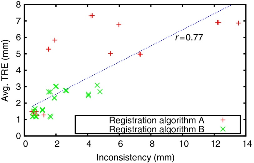
In this section, we introduce our algorithm for CBRR. The goal of the method is to improve pair-wise registrations by minimizing an inconsistency criterion $\mathcal{C}$ defined as the average norm of the inconsistency residuals $r$. Note that consistency is only a necessary condition for correct registrations. This can intuitively be observed when considering the set of identity transforms, which are perfectly consistent but are unlikely to register images properly. This effect can also partly be seen in Fig. 2, where several loops with low inconsistency but substantial registration errors can be observed. We, therefore, additionally constrain the solution of CBRR by penalizing large deviations from the input PTS $\mathcal{R}$ using a function $\mathcal{F}$. This makes use of the fact that a prior PTS $\mathcal{R}$ contains useful information.

Fig. 2.

Inconsistency and target registration error (TRE) for registration loops in four-dimensional (4-D) liver MRI sequences. Each point indicates the inconsistency of one loop of three registrations and the average TRE of those three registrations, and the blue line is a least-square fit with $r=0.77$ denoting the Pearson correlation. For more details on the data and registration algorithms, please see Sec. 4.4.

We define our CBRR algorithm as the minimization of the inconsistency criterion $\mathcal{C}$ for a given input PTS $\mathcal{R}$ obtained using an arbitrary registration method as follows:

$${\mathcal{R}}^{\prime }=\underset{\widehat{\mathcal{R}}}{\mathrm{argmin}}\mathcal{C}(\widehat{\mathcal{R}})+\lambda \mathcal{F}(\mathcal{R},\widehat{\mathcal{R}}),$$ (3)

where ${\mathcal{R}}^{\prime }$ is the rectified PTS and $\lambda$ is the weight controlling its adherence to the prior transformations.

3.1. CBRR Algorithm: Consistency

CBRR minimizes the aggregate inconsistency that is induced by all loops in the set of pair-wise transformations:

$$\mathcal{C}(\widehat{\mathcal{R}})=\sum _{i=1}^N\underset{j\ne i}{\sum _{j=1}^N}\sum _{p\in {\mathrm{\Phi }}_{ij}^m}\sum _{q\in {\mathrm{\Phi }}_{ij}^n}\Vert p-q{\Vert }^2.$$ (4)

A desirable property of such inconsistency criterion is redundancy, which means that each pair-wise registration occurs in the residual of multiple loops. This is an important cue for determining the cause of inconsistencies in a registration. For example, consider a PTS $\mathcal{R}$ where only one transformation ${\mathcal{T}}_{ij}$ has errors which cause inconsistencies. Any consistency loop containing ${\mathcal{T}}_{ij}$ will, therefore, have a non-negative residual $r$, the cause of which cannot easily be located using only information from said loops alone. However, since every transformation other than ${\mathcal{T}}_{ij}$ will also contribute to multiple loops that all have zero residuals, it is, thus, inferable that the cause of inconsistency originates from ${\mathcal{T}}_{ij}$. It is observable that such redundancy is created for any $m$ and $n$ when $m+n>2$. However, the number of summands in Eq. (4) increases exponentially with $m$ and $n$. Furthermore, each transformation composition, especially in longer paths, will require interpolation and, therefore, loses accuracy. This motivates our choice of consistency criterion as (2,1)-consistency (transitivity), where each individual transformation ${\mathcal{T}}_{ij}$ occurs in $3(N-2)$ different loops and the number of transformation compositions is minimal. Then, $\mathcal{C}$ becomes

$$\mathcal{C}(\widehat{\mathcal{R}})=1/Z_{\mathcal{C}}\sum _{i=1}^N\underset{j\ne i}{\sum _{j=1}^N}\underset{k\ne i,j}{\sum _{k=1}^N}\sum _{p\in \mathrm{\Omega }}{\Vert {\widehat{\mathcal{T}}}_{ij}\circ {\widehat{\mathcal{T}}}_{jk}(p)-{\widehat{\mathcal{T}}}_{ik}(p)\Vert }^2,$$ (5)

where $Z_{\mathcal{C}}=MN(N-1)(N-2)$ is a normalization constant (the number of all summands, where $M$ is the total number of all points $p$). This definition also minimizes the number of nonlinear terms in the form of transformation compositions, the importance of which will be explained in Sec. 3.3.

3.2. CBRR Algorithm: Prior

We assume that the initial PTS $\mathcal{R}$ was computed properly and, therefore, carries usable information. This motivates us to penalize large deviations of CBRR solution ${\mathcal{R}}^{\prime }$ from the input PTS. This approach also enables us to avoid degenerate solutions, such as the set of identity transforms. To include similarity-based information in the process, we allow larger deviations from the initial transformation in cases of locally low postregistration similarity. Intuitively, this allows CBRR to limit any negative impact on local registration accuracy while improving consistency. We then define such penalty function $\mathcal{F}$ as follows:

$$\mathcal{F}(\widehat{\mathcal{R}},\mathcal{R})=1/Z_{\mathcal{F}}\sum _{i=1}^N\underset{j\ne i}{\sum _{j=1}^N}\sum _{p\in \mathrm{\Omega }}{\mathrm{\Psi }}_{ij}(p)\Vert {\widehat{\mathcal{T}}}_{ij}(p)-{\mathcal{T}}_{ij}(p){\Vert }^2,$$ (6)

where $p\in \mathrm{\Omega }$ is a (discrete) point, $Z_{\mathcal{F}}=MN(N-1)$ is a normalization constant, and ${\mathrm{\Psi }}_{ij}$ is the local similarity between the transformed image $X_i({\mathcal{T}}_{ij})$ and $X_j$.

We use local normalized cross-correlation (LNCC)³⁴ as the local similarity metric, which was successfully utilized to locally rank segmentation hypotheses in Ref. 35. LNCC can be computed efficiently as follows:

$$\mathrm{LNCC}(X_i,X_j,p)=\frac{\langle X_i,X_j\rangle (p)}{{\sigma }_{X_i}(p){\sigma }_{X_j}(p)},$$ (7)

$$\langle X_i,X_j\rangle (p)=\overline{X_i·X_j}(p)-\overline{X_i}(p)·\overline{X_j}(p),$$ (8)

$$\overline{X}={\mathcal{G}}_{{\sigma }_{\mathcal{G}}}*X,$$ (9)

$${\sigma }_{X_i}^2(p)=\overline{X_i^2}(p)-{\overline{X_i}}^2(p),$$ (10)

where * is the convolution operator and ${\mathcal{G}}_{{\sigma }_{\mathcal{G}}}$ is a Gaussian kernel with standard deviation ${\sigma }_{\mathcal{G}}$. From the LNCC metric, we compute the weights

$${\mathrm{\Psi }}_{ij}={\{1.0-\frac{\mathrm{LNCC}[X_i({\mathcal{T}}_{ij}),X_j]}{2}\}}^{\gamma },$$ (11)

which normalizes LNCC to the range [0,1] and subsequently applies a contrast scaling using $\gamma$. The resulting local weights are shown on an example in Fig. 3.

Fig. 3.

Local normalized cross-correlation (LNCC) weight used for the CBRR regularizer. Shown are target image, deformed source, and LNCC weight computed with $\sigma =4$ mm and $\gamma =10$ for sample pairs from the MRI (left) and CT (right) datasets.

3.3. Casting into a System of Linear Equations

We find a solution for Eq. (3) by casting it as a linear least-squares optimization problem, for which efficient large-scale algorithms exist. The only nonlinear term is the transformation composition in Eq. (5), which we approximate as follows:

$${\widehat{\mathcal{T}}}_{ij}\circ {\widehat{\mathcal{T}}}_{jk}-{\widehat{\mathcal{T}}}_{ik}={\widehat{\mathcal{D}}}_{ij}({\widehat{\mathcal{T}}}_{jk})+{\widehat{\mathcal{D}}}_{jk}-{\widehat{\mathcal{D}}}_{ik},$$ (12)

$$\approx {\widehat{\mathcal{D}}}_{ij}({\mathcal{T}}_{jk})+{\widehat{\mathcal{D}}}_{jk}-{\widehat{\mathcal{D}}}_{ik},$$ (13)

by substituting the unknown true transformation ${\widehat{\mathcal{T}}}_{jk}$ in Eq. (12) with the observed transformation ${\mathcal{T}}_{jk}$ when it is used to deform the displacement field ${\widehat{\mathcal{D}}}_{ij}$.

This allows us to rewrite the minimization problem in the form of ${\mathbf{x}}^{\prime }=\underset{\mathbf{x}}{\min }{|\mathbf{A}\mathbf{x}-\mathbf{b}|}^2$, where $\mathbf{x}$ is the column vector of all grid-point displacement variables for all transformations in $\widehat{\mathcal{R}}$. Then, $\mathbf{x}$ has $MN(N-1)$ entries and has the form

$$\mathbf{x}={[{\widehat{\mathcal{D}}}_{\mathrm{1,2}}(p_1),\cdots ,{\widehat{\mathcal{D}}}_{ij}(p_m),\cdots ,{\widehat{\mathcal{D}}}_{N-1,N}(p_M)]}^T.$$ (14)

The matrix $A$ and the vector $b$ can be decomposed into two parts $A_{\mathcal{C}}$ and $b_{\mathcal{C}}$ for the consistency criterion and $A_{\mathcal{F}}$ and $b_{\mathcal{F}}$ for the regularization term:

$${\mathbf{x}}^{\prime }=\underset{x}{\min }{\left|\right[\begin{array}{c}{A}_{\mathcal{C}}\\ A_{\mathcal{F}}\end{array}]\mathbf{x}-[\begin{array}{c}{b}_C\\ b_{\mathcal{F}}\end{array}\left]\right|}^2.$$ (15)

Each row of $A_{\mathcal{C}}$ consists of 0’s and $\pm 1$’s such that multiplication with $\mathbf{x}$ yields one of the summands of the consistency criterion. The locations of the nonzero entries correspond to the locations of the respective displacements in the vector $\mathbf{x}$ and can be calculated with the help of an indexing function idx() that returns the index of displacement $p$ in transformation ${\mathcal{T}}_{ij}$ as follows:

$$\mathrm{idx}:{\mathbb{N}}^3\to \mathbb{N}:\mathrm{idx}(i,j,p)\to \{1,\dots ,MN(N-1)\}.$$ (16)

Then, each row $r$ of $A_c$ corresponding to a consistency term ${\widehat{\mathcal{D}}}_{ij}[{\mathcal{T}}_{jk}(p)]+{\widehat{\mathcal{D}}}_{jk}(p)-{\widehat{\mathcal{D}}}_{ik}(p)$ has the following entries in column $c$:

$$A_{\mathcal{C}}(r,c)=\{\begin{array}{cc}1,& \text{if}c=\mathrm{idx}[i,j,{\mathcal{T}}_{jk}(p)]\mathrm{or}c=\mathrm{idx}[j,k,p]\\ -1,& \mathrm{if}c=\mathrm{idx}(i,k,p)\\ 0,& \text{otherwise}.\end{array}$$ (17)

All corresponding entries in $b_{\mathcal{C}}$ are then zero, since we want the inconsistency to vanish. When ${\mathcal{T}}_{jk}(p)$ is not on a grid point, we use linear interpolation:

$${\widehat{\mathcal{D}}}_{ij}[{\mathcal{T}}_{jk}(p)]+{\widehat{\mathcal{D}}}_{jk}(p)-{\widehat{\mathcal{D}}}_{ik}(p)\approx [\sum _{p^{\prime }\in \mathcal{N}[{\mathcal{T}}_{jk}(p)]}\nu (p^{\prime })·{\widehat{\mathcal{D}}}_{ij}(p^{\prime })]+{\widehat{\mathcal{D}}}_{jk}(p)-{\widehat{\mathcal{D}}}_{ik}(p),$$ (18)

where $\mathcal{N}$ returns the grid neighborhood of a nongrid point, and $\nu$ computes the interpolation weights. Thus, such consistency-expressing rows in $A_{\mathcal{C}}$ can contain up to 10 nonzero elements in 3-D, where the first nongrid point is interpolated from eight neighboring grid points.

$A_{\mathcal{F}}$ is a square, diagonal matrix such that the multiplication of one row of $A_{\mathcal{F}}$ with $\mathbf{x}$ and subtraction of the corresponding entry of $b_{\mathcal{F}}$ yields one of the prior terms $\lambda {\mathrm{\Psi }}_{ij}(p){\widehat{\mathcal{D}}}_{ij}(p)-\lambda {\mathrm{\Psi }}_{ij}(p){\mathcal{D}}_{ij}(p)$ being minimized. In the same notation as above, this can be expressed as

$$A_{\mathcal{F}}(r,c)=\{\begin{array}{ll}\lambda {\mathrm{\Psi }}_{ij}(p),& \mathrm{if}r=c\\ 0,& \text{otherwise}\end{array};b_{\mathcal{F}}(c)=\lambda {\mathrm{\Psi }}_{ij}(p){\mathcal{D}}_{ij}(p);\text{with}c=\mathrm{idx}(i,j,p).$$ (19)

3.4. Iterative Refinement

In order to improve the approximation in Eq. (13), we employ a fixed point iterative update scheme. In each iteration $t$, a new PTS ${\mathcal{R}}^t$ is computed, where ${\mathcal{R}}^0$ is the CBRR initialization from a prior registration. The estimate of the last iteration is then used for the approximation in Eq. (13) as follows:

$${\mathcal{T}}_{ij}^t\circ {\mathcal{T}}_{jk}^t-{\mathcal{T}}_{ik}^t\approx {\mathcal{D}}_{ij}^t({\mathcal{T}}_{jk}^{t-1})+{\mathcal{D}}_{jk}^t-{\mathcal{D}}_{ik}^t.$$ (20)

This allows the approximation to become more accurate as the difference between ${\mathcal{T}}^{t-1}$ and ${\mathcal{T}}^t$ becomes smaller. The iterative process can also be used to update the prior term. Since we assume that the input registration contains errors, adhering too strongly to it might deteriorate the results of the algorithm. A straightforward way to check for improvements during the iterations is to compare the local postregistration similarities. We, therefore, recompute the local similarity weights ${\mathrm{\Psi }}^t$ after every iteration and keep track of the locally best encountered value along with the corresponding displacement.

$${({\mathrm{\Psi }}^{\text{best}},{\mathcal{D}}^{\text{best}})}_{ijp}=\{\begin{array}{cc}{({\mathrm{\Psi }}^t,{\mathcal{D}}^t)}_{ijp},& \text{if}{\mathrm{\Psi }}_{ij}^t(p)>{\mathrm{\Psi }}_{ij}^{\text{best}}(p)\\ {({\mathrm{\Psi }}^{\text{best}},{\mathcal{D}}^{\text{best}})}_{ijp},& \text{otherwise},\end{array}$$ (21)

where we moved the subindices outside of the tuples for readability. Then we change the prior terms in Eq. (6) to penalize differences from these current best estimates.

$$\mathcal{F}(\widehat{\mathcal{R}},{\mathcal{R}}^{\text{best}})=1/Z_{\mathcal{F}}\sum _{i=1}^N\underset{j\ne i}{\sum _{j=1}^N}\sum _{p\in \mathrm{\Omega }}{\mathrm{\Psi }}_{ij}^{\text{best}}(p)\Vert {\widehat{\mathcal{D}}}_{ij}(p)-{\mathcal{D}}_{ij}^{\text{best}}(p){\Vert }^2.$$ (22)

3.5. Implementation

The number of equations grows with the cube of the number of images, $N$, and linearly with the number of pixels, $M$. However, efficient algorithms for solving large-scale linear least-squares problems exist. We chose the MATLAB® minFunc³⁶ package for its computation and memory efficiency, particularly when dealing with large sparse matrices. In particular, we use the provided limited-memory Broyden–Fletcher–Goldfarb–Shanno solver with a fixed number of 100 iterations. Furthermore, it can be observed that the rows of linear equations corresponding to each principal displacement axis are independent from other axes. Consequently, such equations are separable and each displacement direction can be solved individually, reducing the problem size to half in 2-D and a third in 3-D. Note that these separately solved individual axes still interact with each other in the iterative scheme when the transformation from the previous iteration is used to index current displacements.

Despite the above-mentioned implementation optimizations to reduce memory complexity, solving Eq. (3) at the pixel level is prohibitive mostly due to memory demand. We, therefore, solve our CBRR problem on a coarse grid for efficiency and then interpolate the results. To this end, $\mathcal{R}$ and $\mathrm{\Psi }$ need to be downsampled, leading to information loss which we aim to minimize by using the following full-resolution registration estimates. Let ${\mathcal{R}}_{\text{low}}$ be the downsampled original PTS. The rectified PTS ${\mathcal{R}}_{\text{low}}^{\prime }$ will then be at the same resolution and can be used to estimate the update field ${\mathrm{\Delta }}_{\text{low}}={\mathcal{R}}_{\text{low}}-{\mathcal{R}}_{\text{low}}^{\prime }$. We then upsample ${\mathrm{\Delta }}_{\text{low}}$ to the original resolution and subsequently obtain ${\mathcal{R}}^{\prime }=\mathcal{R}-\mathrm{\Delta }$. This yields registration estimates with the local details preserved, while the local similarities $\mathrm{\Psi }$ are being computed from the full-resolution registrations.

The overall algorithm then works as shown in Algorithm 1. Convergence is achieved when the relative change of residual inconsistency is $<1\%$. The remaining free parameters consist of the regularizer weight $\lambda$, the width of LNCC window $\sigma$, and the exponent $\gamma$.

Algorithm 1.

Outline of the proposed consistency-based registration rectification algorithm.

Data:$\mathcal{R}$, $\mathcal{X}$, $\lambda$, $\gamma$, $\sigma$

Result:${\mathcal{R}}^{\prime }$

$t\leftarrow 0$

${\mathcal{R}}^0\leftarrow \mathcal{R}$

whilenot-convergedand$t<t_{\max }$do

Compute ${\mathrm{\Psi }}^t$ using Eqs. (7)–(11)

Update ${\mathrm{\Psi }}^{\text{best}}$ and ${\mathcal{D}}^{\text{best}}$ according to Eq. (21)

Downsample ${\mathcal{R}}^t$ and ${\mathrm{\Psi }}^t$

forall theaxes$d$do

Form matrix $A_d$ and vector $b_d$ using Eqs. (17)–(22)

${\mathcal{R}}_d^t=\min {|A_{d}x-b_d|}^2$

end

${\mathcal{R}}^t\leftarrow {\cup }_d{\mathcal{R}}_d^t$

Upsample ${\mathcal{R}}^t$

$t\leftarrow t+1$

end

${\mathcal{R}}^{\prime }\leftarrow {\mathcal{R}}^t$

4. Experimental Results

We evaluated our method in three experiments. We first present a controlled environment using synthetic data where known ground truths exist in order to better demonstrate our method. Subsequently, we present our results on two clinical datasets.

4.1. Synthetic Images

We first evaluated our method using a fully synthetic setup where images, registrations, and registration errors were controlled. Nine $199\times 199{\mathrm{px}}^2$ images were created by randomly deforming a reference image and adding 50% SNR noise. We used three different sets of random deformations with varying complexity. To generate smooth, large-scale deformations, we randomly sampled b-spline control grid parameters of an 8×8 grid. To ensure diffeomorphisms, the parameters were uniformly sampled from $[-0.4s,\dots ,0.4s]$, where $s$ is the control grid spacing.³⁷ More complex transformations were generated by using the same process on $20\times 20$ and $50\times 50$ b-spline control grids. We then created three sets of ground-truth transformations, the first using the transformations from the $8\times 8$ grid, the second by composing the transformations from the $20\times 20$ grids onto the first, and the last by composing the transformations from the $50\times 50$ grid onto the second. Pair-wise registrations were then analytically computed by inversion and composition as follows: Let ${\mathcal{T}}_{ri}$ denote the transformation from reference $r$ to an image $i$. The pair-wise transformation ${\mathcal{T}}_{ij}$ can then be computed as

$${\mathcal{T}}_{ij}={\mathcal{T}}_{ri}\circ {\mathcal{T}}_{rj}^{-1},$$ (23)

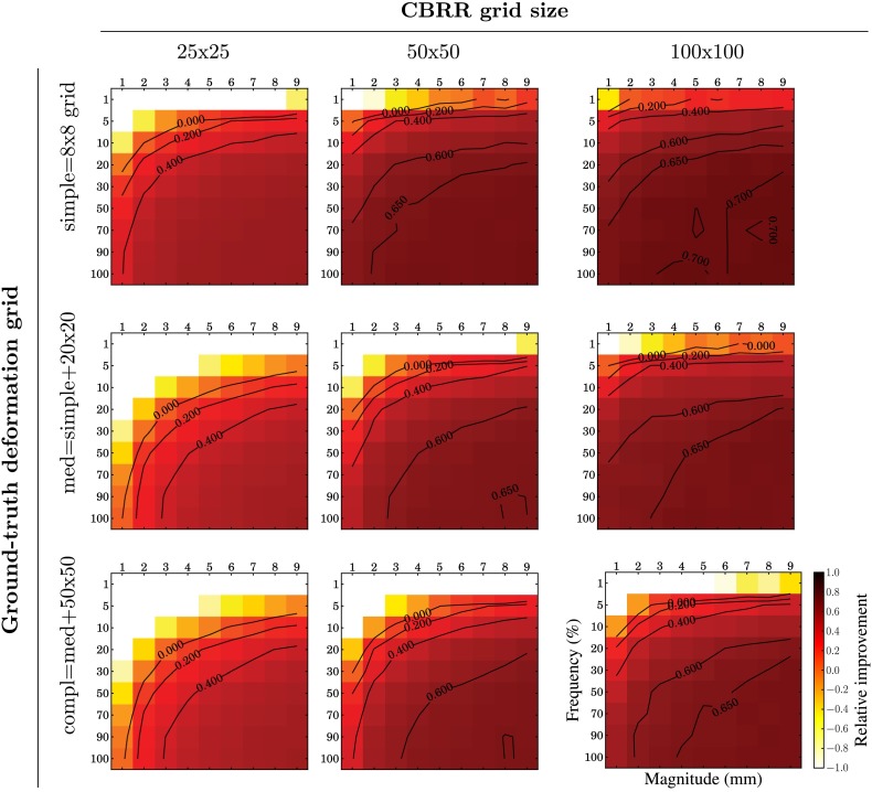
as described in Ref. 26. We then randomly generated errors for each pair-wise transformation as follows: Of a $20\times 20$ b-spline grid, each control point has a varying likelihood $f$ between 1 and 10% to have an error that was uniformly sampled from a variable range $r\in \{1,\dots ,9\}$ and then added to the ground-truth transformations. Each set of parameters $f$ and $r$ then creates a separate PTS, on which we ran CBRR with different grid resolutions. We then compute the relative improvement of the average transformation error (ATE), which is the mean of the Euclidean distance between ground-truth displacements and error displacements as $1.0-{\mathrm{ATE}}_{\mathrm{CBRR}}/{\mathrm{ATE}}_{\mathrm{err}}$, where ${\mathrm{ATE}}_{\mathrm{err}}$ is the ATE of the input PTS. The resulting improvements can be seen in Fig. 4. It can be observed that CBRR can correct a substantial fraction of errors, especially for frequent and large magnitude errors. However, infrequent and small errors cannot be corrected well, which is likely due to CBRR’s relatively coarser grid resolution and additionally due to the quadratic penalty that does not penalize very small changes to the input transformations. This results in small, new errors, which, on average, can be larger than the errors of the original input registration, even though they are very small in absolute terms. CBRR, especially when using a coarse grid, is also challenged by complex underlying true transformations. In those cases, however, a substantial fraction of large deformation errors can still be corrected, and the performance can be improved using higher-resolution grids.

Fig. 4.

Relative improvement using CBRR on synthetic data using random ground-truth deformations of varying complexity, additive random errors with variable magnitude and frequency, and varying CBRR grid resolution.

4.2. 2-D MR Images

For the second experiment, we simulated medical images with known correspondences. We used 19 mid-saggital slices of brain MRI with $481\times 374{\mathrm{px}}^2$ resolution and isotropic spacing of 0.3 mm. In order to obtain a dataset with existing and known dense correspondences, we generated such data using Markov random field (MRF) based registration³⁸ as shown in Fig. 5. We then used the well-known diffeomorphic demons algorithm³⁹ and an MRF-based algorithm³⁸ to mutually re-register all 19 images, resulting in 342 registrations for each method. We solved CBRR separately for both of these sets using a coarse grid with 2.4 mm spacing (downsampling the input PTS by a factor of 8).

Fig. 5.

Data generation for the two-dimensional (2-D) MR experiment. (a) First, image $X_1$ is registered to the remaining images $X_i$, resulting in transformations ${\mathcal{T}}_{1,i}$. (b) Then, $X_1$ is deformed using the estimated transformation and 50% SNR Gaussian noise ($\zeta$) is added, generating new images $X_i^{\prime }$. Pairwise transformations $T_{i,j}$ between all $X_i^{\prime }$ are known analytically through the registrations from $X_1$. (c) The image set $\{X_1,X_2^{\prime },\dots ,X_N^{\prime }\}$ is then used as the experimental dataset and the known dense correspondences ${\mathcal{T}}_{i,j}$ as the ground truth in evaluation.

We first evaluate different choices of $\lambda$ and $\gamma$, the results of which are presented in Fig. 6(a). $\sigma$ was fixed to 4 mm. While a small improvement can even be seen without using the local weights ($\gamma =0$), the performance of CBRR improves substantially for appropriate choices for those parameters ($\gamma =10$, $\lambda =0.5$), which we use throughout all remaining experiments. Note that in the limit cases, CBRR either finds the identity transforms (without any regularization) or the input transforms. We further evaluate how the number of images affects CBRR performance, where results can be seen in Fig. 6(b). A convergence pattern can be observed from about eight images onward.

Fig. 6.

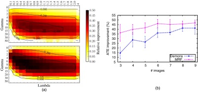
(a) CBRR performance with changing regularization for (b) relative ATE improvement with increasing demons (top) and MRF (bottom) registration. (b) Relative ATE improvement using CBRR with an increasing number of 2D MR images. Each experiment is repeated 10 times with randomly selected images. The standard deviation of the results is shown by the error bars.

Quantitative results by comparing with the analytically computed ground truth are given in Table 1. It is observed that ATE improves by $>45\%$ while the inconsistency $\mathcal{C}$ is reduced considerably. We show one example case for each registration method in Fig. 7 (left), where CBRR is seen to improve the original registration in both cases.

Table 1.

Average transformation error (ATE), inconsistency $\mathcal{C}$, and Pearson correlation $\rho$ of estimated and true registration error magnitude for the two-dimensional MRI experiments using simulated transformations before and after using consistency-based registration rectification (CBRR). We also compare CBRR to locally averaged weighting (LWA), an earlier version of this work [correcting local errors using registration consistency (CLERC)] presented in Ref. 31, and assessing quality using image registration circuits (AQUIRC),¹⁹ which computes a dimensionless estimate of registration error, which can be correlated with the true error.

	Demons			Markov random field (MRF)
	ATE	$\rho$	$\mathcal{C}$	ATE	$\rho$	$\mathcal{C}$
Registration	3.50	—	2.53	1.92	—	1.85
+ LWA	2.34	0.60	1.78	1.83	0.69	1.87
+ CLERC (Ref. 31)	2.66	0.74	0.86	1.28	0.85	0.65
+ CBRR	1.64	0.84	0.35	0.88	0.91	0.22
+ AQUIRC (Ref. 19)	—	0.47	—	—	0.64	—

Note: Bold numbers indicate best results in each category.

Fig. 7.

CBRR of Markov random field (MRF) (top) and demons (bottom) registration on the 2-D MRI data. Shown are, from left to right, target image, deformed source, true registration error, error of rectified registration, and the source image deformed by the rectified registration. The hue of the color in the error visualizations indicates its orientation, while the saturation corresponds to the error magnitude.

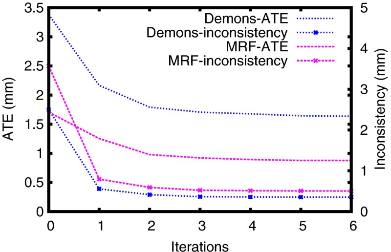
We compare CBRR to straightforward locally weighted averaging (LWA), which fuses all indirect transformations ${\mathcal{T}}_{ik}\circ {\mathcal{T}}_{kj}$ and the direct transformation ${\mathcal{T}}_{ij}$. The local weights are computed using the same LNCC technique as in CBRR, but parameters have been tuned separately ($\sigma =8$, $\gamma =30$) to not put the LWA method at a disadvantage. We also compared CBRR to Correcting Local Errors using Registration Consistency (CLERC),³¹ which is a preliminary version of the technique presented in this paper. The main difference is that CLERC uses no iterative updates and a different numerical solver. This difference can partly be observed in Fig. 8, where the CLERC results shown in Table 1 are similar to CBRR after the first iteration, with remaining differences caused by a different numerical solver. CBRR then typically converges after about five to six iterations. As shown in Table 1, CBRR outperforms CLERC and LWA in all metrics for all experiments. We elaborate on the differences between CLERC and CBRR later in Sec. 4.5. We also compare our method to our own implementation of assessing quality using image registration circuits (AQUIRC),^19,20 which computes a dimensionless measure of local registration error magnitude which can be correlated with the true local error magnitudes. It is observed that the magnitude of the updates computed by CBRR correlate substantially stronger with the true error magnitudes in comparison to AQUIRC.

Fig. 8.

Improvements through CBRR over multiple iterations.

4.3. 3-D CT Segmentation

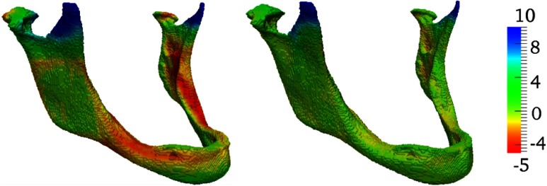
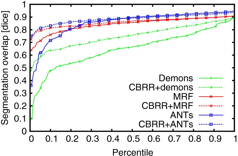
The next experiment was performed using a clinical dataset of 15 3-D CT head scans from different individuals, with $160\times 160\times 129{\text{pixel}}^2$ resolution and 1 mm spacing. All images were mutually registered using demons-, MRF- and advanced normalization tools (ANTs)⁴⁰-based registrations, yielding a total of 210 transformations for each registration algorithm. Postregistration target registration error (TRE) was computed using 12 manually placed landmarks, which were placed at anatomically identifiable locations on the jawbone and the skull for all images. In addition to TRE, we also evaluated anatomical overlap of manually segmented mandibles using Dice’s coefficient, mean surface distance, and Hausdorff distance. Note that, in contrast to the above experiments, in this current experiment with actual interpatient registrations, neither consistency nor dense correspondences can be guaranteed. Indeed, in these 3-D CTs, the presence and number of teeth vary substantially among the scanned individuals. We solved CBRR using a coarse grid with 8 mm spacing using the same parameters as the 2-D MRI experiment above ($\lambda =0.5$, $\sigma =4\mathrm{mm}$, $\gamma =10$). Results are given in Table 2, in which a significant ($\rho <5\%$) improvement in both TRE and segmentation metrics using CBRR can be observed. A larger improvement is observed for the demons registrations, which has a poorer initial performance. We show an example of corresponding postregistration and post-CBRR segmentations in Fig. 9, and the distributions of segmentation overlap before and after CBRR can be seen in Fig. 10. Here, it is clearly observable that CBRR substantially improves the worst-case segmentation quality induced by the input PTS, while best-case Dice overlap can be slightly reduced. In the case of the demons registration algorithm, segmentation quality is substantially improved for all registrations.

Table 2.

Quantitative evaluation of CBRR and comparison to group-wise registration on the three-dimensional (3-D) CT dataset. Mean TRE, mean surface distance (MSD), Hausdorff distance (HD), and inconsistency $\mathcal{C}$ are given in mm.

	3-D CT
	TRE	Dice	MSD	HD	$\mathcal{C}$	Total run time (h)
Reg-demons	$9.25\pm 4.22$	$0.65\pm 0.15$	$1.27\pm 1.19$	$17.86\pm 8.83$	8.14	140
+ CBRR	$7.16\pm 2.19$	$0.75\pm 0.09$	$0.58\pm 0.36$	$14\pm 5.65$	1.07	$+2.5$
Reg-MRF	$5.25\pm 1.95$	$0.84\pm 0.06$	$0.34\pm 0.29$	$11.43\pm 4.86$	5.67	39
+ CBRR	$\mathbf{4.66}\pm 1.20$	$0.86\pm 0.03$	$0.22\pm 0.10$	$9.72\pm 3.65$	1.12	$+2.5$
Reg-ANTs	$6.02\pm 3.35$	$0.85\pm 0.11$	$0.49\pm 0.68$	$12.27\pm 5.99$	6.43	105
+ CBRR	$4.70\pm 1.60$	$\mathbf{0.89}\pm 0.04$	$\mathbf{0.17}\pm 0.12$	$\mathbf{8.79}\pm 3.48$	1.13	$+2.5$
Group-wise reg.	$8.1\pm 2.86$	$0.75\pm 0.10$	$0.97\pm 0.61$	$22.64\pm 4.30$	0.0	26

Note: ANTs, advanced normalization tools; Bold numbers indicate best results in each category.

Fig. 9.

Surface distance of ground-truth jawbone segmentation to (a) MRF registered source and (b) subsequent CBRR. Best viewed in color.

Fig. 10.

Segmentation overlap percentiles on the three-dimensional (3-D) CT dataset. Each data point shows the maximum Dice coefficient for a given percentage of the 210 total pair-wise registrations.

We also compared CBRR to a traditional group-wise registration method. We used the medical image registration toolkit which is publicly available.⁴¹ It implements a well-known group-wise registration method in which the images are iteratively registered to an evolving group mean. We used the default parametrization, which utilizes residual complexity⁴² as the similarity measure. The results for this comparison are given in Table 2. While the group-wise registration outperforms the plain pair-wise demons algorithm, using CBRR is seen to yield the best result in all cases and for all evaluation metrics.

4.4. Four-Dimensional Liver MRI Motion Estimation

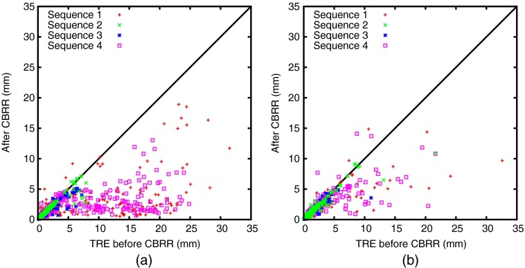
We also evaluated our method on motion estimation from four-dimensional (4-D) MRI. Images of a 4-D sequence are typically registered to one reference frame, e.g., exhale, and pair-wise transformations and subsequently an estimate of the motion can be inferred from those.²⁶ Other studies have shown that it is beneficial to initialize such registrations with the transformation of the previous image in the sequence.⁴³ Using CBRR, we compute all pair-wise registrations for all images in a sequence, which then includes both the direct registrations between the reference frame and the remaining frames, as well as the sequential registrations. CBRR can then update the resulting PTS where consistent correspondences are guaranteed to exist. We use four sequences of the abdomen for our evaluation, which were recorded using the technique described in Ref. 44. Each sequence contains 11 breathing phases (images) with a spatial resolution of $1.37\times 1.37\times 4{\mathrm{mm}}^3$, $\sim 370\mathrm{ms}$ temporal resolution, and a mean image size of $164\times 189\times 23\text{voxels}$. Fifty-two landmarks were placed manually at anatomically identifiable positions, such as ribs, vertebrae and vessel bifurcations in the liver, kidneys, and lungs, for one exhale and two inhale images in each sequence. Registration quality can then be assessed in terms of mean TRE between the ground-truth and transformed landmarks for all image pairs where landmarks are available. We used two registration methods for each sequence: ANTs⁴⁰ as it delivers state-of-the-art results on many public datasets, and a parametric total variation (PTV) registration method, which was specifically developed considering the sliding motion that occurs during breathing in abdominal imaging.⁴⁵ Figure 11 shows one CBRR loop of exhale-inhale-inhale using PTV, and the resulting dense inconsistency and extrapolated TRE before and after CBRR, which was run on deformations that were downsampled by a factor of 4. The grid spacing was kept as isotropic as possible, resulting in a spacing of $5.48{\mathrm{mm}}^3$. CBRR parameters were the same as for the other experiments with $\gamma =10$, $\sigma =4$, and $\lambda =0.5$. Table 3 shows quantitative results, where a substantial and significant ($\rho <5\%$) improvement in TRE can be observed. Interestingly, the CBRR TRE results of both registration methods are very similar to each other, despite the substantial difference in input TRE. Figure 12 visualizes the change in registration error per landmark for both registration methods before and after using CBRR. It can be observed that the worst-case performance is especially improved, reducing the maximum TRE by up to 60%.

Fig. 11.

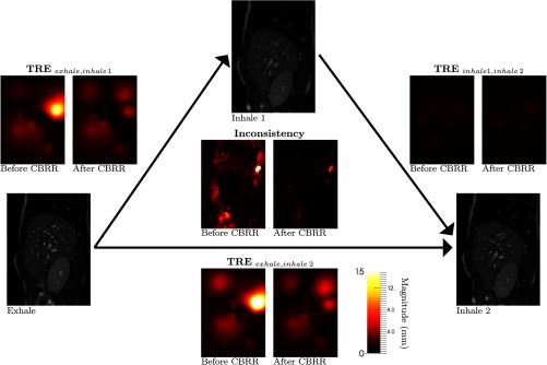
Inconsistency and TRE of one loop of sequence 1 before and after using CBRR for the parametric total variation registration method. Mid-sagittal slices are shown for MRIs, inconsistency, and TRE extrapolated using thin-plate splines. CBRR was computed on a longer sequence using 11 images and 110 registrations in total.

Table 3.

Quantitative evaluation of CBRR on the four-dimensional liver MRI sequences. The average run time is the average time required to process one of the sequences with 11 breathing phases of 3-D MR.

	Average TRE per sequence (mm)				Total mean	Avg. run time (h)
	1	2	3	4
Without reg	$10.99\pm 6.58$	$3.91\pm 1.92$	$5.64\pm 3.29$	$11.12\pm 6.26$	$7.95\pm 7.73$	—
Reg-ANTs	$5.95\pm 7.20$	$1.49\pm 1.36$	$1.26\pm 1.24$	$6.30\pm 6.70$	$3.75\pm 5.50$	10
+ CBRR	$2.31\pm 2.83$	$1.42\pm 1.17$	$1.13\pm 0.92$	$2.27\pm 1.85$	$1.81\pm 1.91$	$+3$
Reg-PTV	$2.50\pm 3.51$	$1.58\pm 1.85$	$1.18\pm 1.02$	$2.89\pm 3.28$	$2.04\pm 2.70$	2
+ CBRR	$1.94\pm 1.83$	$1.47\pm 1.41$	$1.10\pm 0.77$	$2.20\pm 1.89$	$1.68\pm 1.60$	$+3$

Note: PTV, parametric total variation.

Fig. 12.

TRE before and after CBRR on the 4D Liver MRI sequences for (a) ANTs and (b) PTV deformable registration. Each point shows the error for a single landmark before ($x$ axis) and after ($y$ axis) CBRR. Note that points below the $y=x$ line indicate a reduction in error using CBRR.

4.5. Discussion

We experimentally demonstrated that CBRR improves (2,1)-consistency on a variety of different input data and using different pair-wise registration methods. In addition to the consistency improvement, CBRR was shown to yield improved transformations in terms of average transformation error, TRE, and segmentation overlap. As can be seen in Fig. 10, such improvements mostly affect poorer pair-wise registrations (lower percentile) in the case of a relatively well-performing initial registration, e.g., using MRFs. In contrast, if the initial registration is poorer as in demons registration algorithm, the Dice overlap increases among all but the top percentiles. This is attributed to the higher initial inconsistency of poorer registrations, which yields more space for improvements via registration rectification.

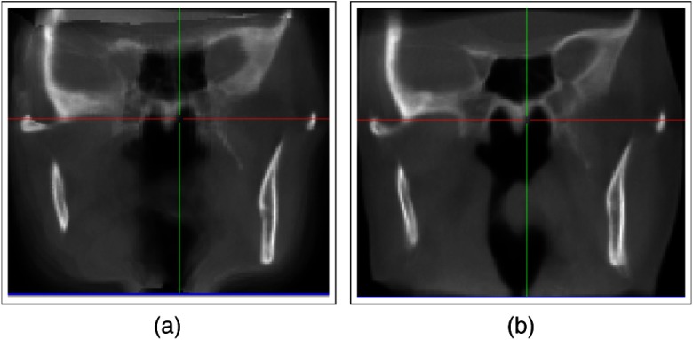
Besides an improvement in pair-wise alignment, the results of CBRR are particularly interesting for group-wise methods, such as atlas generation. As shown in Table 2, CBRR can outperform group-wise registration quantitatively. A typical qualitative result of group-wise registration is the resulting mean image, which represents the center of the distribution. Here, a sharp mean image is an indicator for the successful alignment of all images to such a mean. We present mean images using registrations from CBRR and group-wise registrations in Fig. 13. Since CBRR does not directly return the center of the distribution, the images are in the reference space of one randomly chosen image for better comparison. It can be seen that the CBRR mean is much sharper than the group-wise mean, indicating that group-wise registration could not align the images satisfactorily in this task.

Fig. 13.

Mid-coronal slices of the mean images of the 3-D CT dataset for (a) group-wise and (b) CBRR registration. For CBRR, one image was chosen as reference to which all images were aligned for averaging. We deformed the group-wise mean to the same image to allow a better comparison.

Note that CBRR yields satisfactory results in all tests with a uniform parametrization. Note that further experiment-specific improvement is possible, in particular by adjusting $\lambda$ to incorporate prior knowledge on the expected error. Different choices of the local similarity metric can also be beneficial, especially for multimodal data.

CBRR can also be interpreted as a detection method for inconsistency-based registration errors. Based on the difference between the estimated and the original registrations, one can estimate local error magnitudes. These estimations can be evaluated through ground-truth local-error magnitudes for experiments for which those are known. This allows for a comparison with AQUIRC,^19,20 which computes a dimensionless measure of local error magnitude based on (3,0)-consistency. We used our own implementation of their technique, the results of which were presented in Table 1. Note that CBRR could also be adapted to utilize (3,0)-consistency, but would require an additional approximation (c.f. Sec. 3.3) for the additional transformation composition, which would make the implementation more complicated and the solution less robust. The error magnitudes estimated by CBRR correlate more strongly with the true error magnitudes in comparison to AQUIRC, in addition to surpassing our earlier algorithm CLERC.³¹ Additionally, both CLERC and CBRR estimate actual error vectors in contrast to the dimensionless measure being reported by AQUIRC. The difference in performance between CBRR and CLERC can mainly be explained through the additional iterative refinement in CBRR, which improves the approximation in Eq. (12). An additional benefit of CBRR is that it requires that only registration variables be estimated, in contrast to registration and error variables in CLERC. This makes it computationally more efficient and easier to parametrize since one less parameter is required.

Still, the bottleneck of the proposed CBRR algorithm is its large memory requirement since all the displacement variables are estimated simultaneously. This contrasts with the AQUIRC approach,¹⁹ which can independently solve for the error at every spatial location. In our experiments, the memory utilization reached up to 15 GB for the 3-D CT segmentation experiment. The main factor for this is the number of nonzero entries in $A$, which is proportional to $N^{3}M$, where $M$ denotes the number of coarse grid points. Note that we keep only the downsampled pair-wise registrations in memory while reloading the full-resolution registrations only on demand. We implemented our CBRR prototype in C++/ITK. Constructed systems of equations are solved using the minFunc solver called via the MATLAB® engine interface for C++. The equation system itself is not particularly large in memory, requiring $\sim 6\mathrm{GB}$ including all auxiliary variables for the 15 3-D CT image problem. However, a significant memory overhead is needed in MATLAB® for passing and solving the problem. Therefore, using a dedicated C++ solver might be one approach to reducing memory demands. Additionally, our experiments showed that satisfactory results can be already achieved with a limited number of images (c.f. Fig. 6). For instance, reducing the number of images from 15 to 7 in the 3-D case would reduce the memory requirements by a factor of 8. One advantage of CBRR is the speed with which all pair-wise registrations are updated. One full iteration, which updates 210 3-D registrations, takes about 30 min, including the computation of pair-wise local similarities. This is $\sim 80$ times faster than computing all the pair-wise registrations using MRFs. Since the proposed approach is likely to be used in an offline fashion, it would be reasonable to trade off run time for decreased memory usage, thereby also allowing for more images and/or higher-resolution transformations.

A strong point of CBRR is that it is independent of the used registration algorithm and imposes no restrictions on the spatial smoothness of the transformations. This also enables its application in challenging scenarios as in registration with sliding motion, as can be seen from the results on the 4-D MRI experiment, where substantial improvements are seen both for a smooth (ANTs) and for a sliding-motion enabled registration method.

5. Conclusions

We presented a population-based method for refining pair-wise registrations by reducing their inconsistency (CBRR, software will be made available⁴⁶). By formulating the task as a linear least-squares problem, we obtain an efficient algorithm that is able to resolve such inconsistencies in groups of up to 15 3-D images simultaneously, which is, to the best of our knowledge, not possible with any other technique. In contrast to group-wise registration, our method is arguably better suited for interpatient registration, as correspondences need not be perfect across all images. Instead, a trade-off is achieved, balancing group-wise consistency and pair-wise visual similarity. Experimentally, our approach was shown to be able to not only increase consistency, but also improve segmentation overlap in atlas-based segmentation, and target registration error in both inter- and intrapatient registration, where the latter is an important problem, e.g., for breathing motion estimation.

Biographies

Tobias Gass received his diploma in computer science from RWTH Aachen University, Germany, in 2009 and his PhD in medical image analysis from ETH Zurich, Switzerland, in 2014. From 2009 to 2010, he was a research assistant at the RWTH Aachen University, where he worked on face and optical character recognition. Since 2010, he has been with the Computer Vision Laboratory, ETH Zurich. His research interests include medical image segmentation and registration, and machine learning.

Gábor Székely received his graduate degrees in chemical engineering and applied mathematics and a PhD degree in analytical chemistry in Budapest, Hungary. He is currently full professor of medical image analysis and visualization at the Computer Vision Laboratory, ETH Zurich, Switzerland, where he is involved in the development of image analysis, visualization and simulation methods for computer support of medical diagnosis, therapy, training, and education.

Orcun Goksel received BSc degrees in electrical engineering (2001) and in computer science (2002) from Middle East Technical University, Ankara, Turkey. He received his MASc (2004) and PhD (2009) degrees in electrical and computer engineering at the University of British Columbia, Vancouver, Canada. He is currently an assistant professor at ETH Zurich, Switzerland. His research interests include medical image analysis, image-guided therapy, patient-specific modelling, virtual-reality simulation, ultrasound imaging, and elastography.

References

- 1.Rohlfing T., et al. , “Quo vadis, atlas-based segmentation?,” in Handbook of Biomedical Image Analysis, Suri J. S., Wilson D. L., Laxminarayan S., Eds., pp. 435–486, Springer, US: (2005). [Google Scholar]
- 2.Fischer B., Modersitzki J., “Ill-posed medicine—an introduction to image registration,” Inverse Probl. 24, 1–19 (2008). 10.1088/0266-5611/24/3/034008 [DOI] [Google Scholar]
- 3.Lee S., Wolberg G., Shin S., “Scattered data interpolation with multilevel B-splines,” IEEE Trans. Vis. Comput. Graph. 3(3), 228–244 (1997). 10.1109/2945.620490 [DOI] [Google Scholar]
- 4.Crum W., Griffin L., Hawkes D., “Automatic estimation of error in voxel-based registration,” in Proc. of Medical Image Computing and Computer-Assisted Intervention, pp. 821–828, Springer, Berlin, Heidelberg: (2004). [Google Scholar]
- 5.Schestowitz R. S., et al. , “Non-rigid registration assessment without ground truth,” in Proc. of IEEE Int. Symp. Biomedical Imaging: From Nano to Macro, pp. 836–839, IEEE, Arlington, VA: (2006). [Google Scholar]
- 6.Muenzing S. E. A., et al. , “Supervised quality assessment of medical image registration: application to intra-patient CT lung registration,” Med. Image Anal. 16, 1521–1531 (2012). 10.1016/j.media.2012.06.010 [DOI] [PubMed] [Google Scholar]
- 7.Lotfi T., et al. , “Improving probabilistic image registration via reinforcement learning and uncertainty evaluation,” Lec. Notes Comput. Sci. 8184, 187–194 (2013). 10.1007/978-3-319-02267-3 [DOI] [Google Scholar]
- 8.Crum W., et al. , “Zen and the art of medical image registration: correspondence, homology, and quality,” NeuroImage 20, 1425–1437 (2003). 10.1016/j.neuroimage.2003.07.014 [DOI] [PubMed] [Google Scholar]
- 9.Rohlfing T., “Image similarity and tissue overlaps as surrogates for image registration accuracy: widely used but unreliable,” IEEE Trans. Med. Imaging 31, 153–163 (2012). 10.1109/TMI.2011.2163944 [DOI] [PMC free article] [PubMed] [Google Scholar]
- 10.Robinson D., Milanfar P., “Fundamental performance limits in image registration,” IEEE Trans. Image Process. 13(9), 1185–1199 (2004). 10.1109/TIP.2004.832923 [DOI] [PubMed] [Google Scholar]
- 11.Kybic J., “Bootstrap resampling for image registration uncertainty estimation without ground truth,” IEEE Trans. Image Process. 19, 64–73 (2010). 10.1109/TIP.2009.2030955 [DOI] [PubMed] [Google Scholar]
- 12.Risholm P., et al. , “Bayesian characterization of uncertainty in intra-subject non-rigid registration,” Med. Image Anal. 17, 538–555 (2013). 10.1016/j.media.2013.03.002 [DOI] [PMC free article] [PubMed] [Google Scholar]
- 13.Simpson I. J. A., et al. , “A Bayesian approach for spatially adaptive regularisation in non-rigid registration,” in Proceedings of MICCAI 2013, pp. 10–18, Springer, Berlin, Heidelberg: (2013). 10.1007/978-3-642-40763-5 [DOI] [PubMed] [Google Scholar]
- 14.Muenzing S., et al. , “DIRBoost: an algorithm for boosting deformable image registration,” in Int. Symp. on Biomedical Imaging, pp. 1339–1342, IEEE, Arlington, VA: (2012). [Google Scholar]
- 15.Pennec X., Thirion J.-P., “A framework for uncertainty and validation of 3-D registration methods based on points and frames,” Int. J. Comput. Vis. 25, 203–229 (1997). 10.1023/A:1007976002485 [DOI] [Google Scholar]
- 16.Woods R. P., et al. , “Automated image registration: I. General methods and intrasubject, intramodality validation,” J. Comput. Assist. Tomogr. 22(1), 139–152 (1998). 10.1097/00004728-199801000-00027 [DOI] [PubMed] [Google Scholar]
- 17.Holden M., et al. , “Voxel similarity measures for 3-D serial MR brain image registration,” IEEE Trans. Med. Imaging 19, 94–102 (2000). 10.1109/42.836369 [DOI] [PubMed] [Google Scholar]
- 18.Christensen G. E., Johnson H. J., “Consistent image registration,” IEEE Trans. Med. Imaging 20, 568–582 (2001). 10.1109/42.932742 [DOI] [PubMed] [Google Scholar]
- 19.Datteri R., Dawant B., “Automatic detection of the magnitude and spatial location of error in non-rigid registration,” in Biomedical Image Registration, pp. 21–30, Springer, Berlin, Heidelberg: (2012). [Google Scholar]
- 20.Datteri R. D., et al. , “Validation of a non-rigid registration error detection algorithm using clinical MRI brain data,” IEEE Trans. Med. Imaging 34(1), 86–96 (2015). 10.1109/TMI.2014.2344911 [DOI] [PMC free article] [PubMed] [Google Scholar]
- 21.Datteri R. D., et al. , “Estimation of registration accuracy applied to multi-atlas segmentation,” in MICCAI Workshop on Multi-Atlas Labeling and Statistical Fusion, pp. 78–87 (2011). [Google Scholar]
- 22.Goksel O., et al. , “Estimation of atlas-based segmentation outcome: leveraging information from unsegmented images,” in Proc of IEEE Int. Symp. on Biomedical Imaging, pp. 1203–1206, IEEE; (2013). [Google Scholar]
- 23.Vercauteren T., et al. , “Symmetric log-domain diffeomorphic registration: a demons-based approach,” in Proc. of Medical Image Computing and Computer-Assisted Intervention, pp. 754–761, Springer, Berlin Heidelberg: (2008). [DOI] [PubMed] [Google Scholar]
- 24.Avants B. B., et al. , “Symmetric diffeomorphic image registration with cross-correlation: evaluating automated labeling of elderly and neurodegenerative brain,” Med. Image Anal. 12, 26–41 (2008). 10.1016/j.media.2007.06.004 [DOI] [PMC free article] [PubMed] [Google Scholar]
- 25.Joshi S., et al. , “Unbiased diffeomorphic atlas construction for computational anatomy,” NeuroImage 23(Suppl 1), S151–160 (2004). 10.1016/j.neuroimage.2004.07.068 [DOI] [PubMed] [Google Scholar]
- 26.Skrinjar O., Bistoquet A., Tagare H., “Symmetric and transitive registration of image sequences,” Int. J. Biomed. Imaging 2008, 686875 (2008). 10.1155/2008/686875 [DOI] [PMC free article] [PubMed] [Google Scholar]
- 27.Bhatia K. K., Hajnal J., “Consistent groupwise non-rigid registration for atlas construction,” in Proc. of IEEE Int. Symp. on Biomedical Imaging, pp. 908–911, IEEE; (2004). [Google Scholar]
- 28.Geng X., Kumar D., Christensen G. E., “Transitive inverse-consistent manifold registration,” in Proc. of Information Processing in Medical Imaging, pp. 468–479, Springer, Berlin Heidelberg: (2005). [DOI] [PubMed] [Google Scholar]
- 29.Geng X., “Transitive inverse-consistent image registration and evaluation,” PhD Thesis, University of Iowa (2007). [Google Scholar]
- 30.Glatard T., Pennec X., Montagnat J., “Performance evaluation of grid-enabled registration algorithms using bronze-standards,” Med. Image Comput. Comput. Assist. Interv. 4191, 152–160 (2006). 10.1007/11866763_19 [DOI] [PubMed] [Google Scholar]
- 31.Gass T., Szekely G., Goksel O., “Detection and correction of inconsistency-based errors in non-rigid registration,” Proc. SPIE 9034, 90341B (2014). 10.1117/12.2042757 [DOI] [Google Scholar]
- 32.Christensen G. E., Johnson H. J., “Invertibility and transitivity analysis for nonrigid image registration,” J. Electron. Imaging 12(1), 106–117 (2003). 10.1117/1.1526494 [DOI] [Google Scholar]
- 33.Song J. H., et al. , “Evaluating image registration using NIREP,” Lec. Notes Comput. Sci. 6204, 140–150 (2010). 10.1007/978-3-642-14366-3 [DOI] [Google Scholar]
- 34.Cachier P., et al. , “Iconic feature based nonrigid registration: the PASHA algorithm,” Comput. Vis. Image Underst. 89, 272–298 (2003). 10.1016/S1077-3142(03)00002-X [DOI] [Google Scholar]
- 35.Cardoso M. J., et al. , “Multi-STEPS: multi-label similarity and truth estimation for propagated segmentations,” in IEEE Workshop on Mathematical Methods in Biomedical Image Analysis, pp. 153–158, IEEE; (2012). [Google Scholar]
- 36.Mark S., “Minfunc Unconstrained Differentiable Multivariate Optimization In Matlab,” http://www.cs.ubc.ca/~schmidtm/Software/minFunc.html (2012).
- 37.Rueckert D., et al. , “Diffeomorphic registration using B-splines,” Lec. Notes Comput. Sci. 4191, 702–709 (2006). 10.1007/11866763 [DOI] [PubMed] [Google Scholar]
- 38.Glocker B., et al. , “Dense image registration through MRFs and efficient linear programming,” Med. Image Anal. 12, 731–741 (2008). 10.1016/j.media.2008.03.006 [DOI] [PubMed] [Google Scholar]
- 39.Vercauteren T., et al. , “Diffeomorphic demons: efficient non-parametric image registration,” NeuroImage 45, 61–72 (2009). 10.1016/j.neuroimage.2008.10.040 [DOI] [PubMed] [Google Scholar]
- 40.Avants B., Tustison N., Song G., “Advanced normalization tools (ANTS),” Insight J. 45(1), 1–35 (2009). [Google Scholar]
- 41.Myronenko A., “Groupwise image registration,” 2013, https://sites.google.com/site/myronenko/software (2013).
- 42.Myronenko A., Song X., “Intensity-based image registration by minimizing residual complexity,” IEEE Trans. Med. Imaging 29, 1882–1891 (2010). 10.1109/TMI.2010.2053043 [DOI] [PubMed] [Google Scholar]
- 43.Tanner C., Samei G., Székely G., “Investigating anisotropic diffusion for the registration of abdominal MR images,” in Proc. of IEEE Int. Symp. on Biomedical Imaging, pp. 484–487, IEEE; (2013). [Google Scholar]
- 44.von Siebenthal M., et al. , “4D MR imaging of respiratory organ motion and its variability,” Phys. Med. Biol. 52, 1547–1564 (2007). 10.1088/0031-9155/52/6/001 [DOI] [PubMed] [Google Scholar]
- 45.Vishnevskiy V., et al. , “Total variation regularization of displacements in parametric image registration,” Lec. Notes Comput. Sci. 8676 (2014). 10.1007/978-3-319-13692-9 [DOI] [PubMed] [Google Scholar]
- 46.Computer Vision Lab ETH Zurich, “Software,” http://www.vision.ee.ethz.ch/software/index.en.html (2015).