SimSeq: a nonparametric approach to simulation of RNA-sequence datasets

Abstract

Motivation: RNA sequencing analysis methods are often derived by relying on hypothetical parametric models for read counts that are not likely to be precisely satisfied in practice. Methods are often tested by analyzing data that have been simulated according to the assumed model. This testing strategy can result in an overly optimistic view of the performance of an RNA-seq analysis method.

Results: We develop a data-based simulation algorithm for RNA-seq data. The vector of read counts simulated for a given experimental unit has a joint distribution that closely matches the distribution of a source RNA-seq dataset provided by the user. We conduct simulation experiments based on the negative binomial distribution and our proposed nonparametric simulation algorithm. We compare performance between the two simulation experiments over a small subset of statistical methods for RNA-seq analysis available in the literature. We use as a benchmark the ability of a method to control the false discovery rate. Not surprisingly, methods based on parametric modeling assumptions seem to perform better with respect to false discovery rate control when data are simulated from parametric models rather than using our more realistic nonparametric simulation strategy.

Availability and implementation: The nonparametric simulation algorithm developed in this article is implemented in the R package SimSeq, which is freely available under the GNU General Public License (version 2 or later) from the Comprehensive R Archive Network (http://cran.rproject.org/).

Contact: sgbenidt@gmail.com

Supplementary information: Supplementary data are available at Bioinformatics online.

1 Introduction

Over the past decade, new high-throughput next-generation sequencing technology has become readily available for gene expression profiling of RNA samples. The new next-generation sequencing technology has unseated the previous dominance of microarray technology, offering low sequencing costs, more detailed sequencing information and a wider range of signal detection.

A main focus in the statistical analysis of an RNA-seq dataset is the detection of differential expression. A gene is considered to be differentially expressed (DE) across a set of conditions if the mean gene expression level (as measured by RNA-seq read count) differs among any of the conditions. Otherwise, we say the gene is equivalently expressed (EE) or is a null gene. For the sake of exposition, we assume that the statistical analysis under discussion is on the gene level, though our comments could apply equally well to count datasets involving other genomic features for which counts can be reliably obtained.

1.1 Benchmarks for simulation experiments

Many researchers design simulation experiments to study the efficacy of their proposed methods over a range of differing situations. In the case of RNA-seq data, such studies frequently rely on simulating counts from a known parametric distribution such as negative binomial (NB), with parameters guided by a real RNA-seq dataset. However, datasets simulated in this manner do not necessarily match the complex structure of the RNA-seq datasets they attempt to emulate. In this article, we propose a nonparametric simulation algorithm for the construction of an RNA-seq dataset with two independent treatment groups. The simulated dataset closely matches the complex structure of real RNA-seq data. We refer to this data-based simulation procedure as the SimSeq algorithm.

Data-based simulation procedures have been used to simulate gene expression experiments. A data-based simulation procedure involves subsampling from a large source dataset in such a way that the underlying truth of the dataset is known, e.g. the null hypothesis of no difference in population mean expression is satisfied. Gadbury et al. (2008) proposed a simulation procedure for constructing plasmode microarray datasets from a high dimensional microarray dataset. Nettleton et al. (2008) developed a different data-based simulation method for microarray data to validate a proposed multiresponse permutation procedure for gene set testing. Liang and Nettleton (2010) made use of this same simulation strategy to evaluate a hidden Markov model for microarray data. Robinson and Storey (2014) used a resampling method based on the binomial distribution to determine optimal sequencing depth in an RNA-seq experiment. Love et al. (2014) used a data-based simulation procedure to support their DESeq2 methodology for RNA-seq data analysis. Griebel et al. (2012) developed an RNA-seq simulation procedure that mimics the data generating process. Reeb and Steibel (2013) developed another plasmode simulation algorithm for RNA-seq datasets. Although the concept of data-based simulation in gene expression experiments is not new, the novelty of our proposed method lies in the specific implementation of our nonparametric simulation algorithm for RNA-seq data.

We conduct two simulation studies, one using a standard parametric simulation approach based on NB distributions and the other using our proposed nonparametric simulation algorithm. We do so for a small subset of statistical methods in the literature: DESeq2 (Anders and Huber, 2010; Love et al., 2014), edgeR (McCarthy et al., 2012; Robinson and Smyth, 2007, 2008; Robinson et al., 2010), QuasiSeq (Lund et al., 2012), Voom (Law et al., 2014) and SAMseq (Li and Tibshirani, 2013). Unlike most simulation studies, the main focus of our work is a comparison of simulation methods rather than a comparison of the analysis methods. We are unaware of other RNA-seq simulation studies that conduct a side-by-side comparison of a data-based simulation procedure and a parametric simulation procedure.

We use the average false discovery proportion (FDP) compared with nominal false discovery rate (FDR) as a benchmark of performance for a given statistical method. FDP is defined to be zero whenever no null hypotheses are rejected and is otherwise the number of false positives (type I errors) divided by the number of rejected null hypotheses. The FDR introduced by Benjamini and Hochberg (1995) is the expected value of FDP. Thus, a comparison of average FDP to nominal FDR allows us to empirically evaluate how well an analysis method controls FDR for a given simulation method.

In our simulation experiments, we find that average FDP is typically lower under the standard parametric simulations. Thus, simulation studies based on parametric simulations may give a misleading view of the effectiveness of a proposed statistical method for RNA-seq data analysis. We believe that using the nonparametric SimSeq algorithm gives a more accurate picture of the performance of a given method to detect differential expression while controlling FDR.

2 Preliminaries

2.1 Notation

Let Y be a matrix of RNA-seq read count data, and let y_git be a single read count in Y, where $g=1,\dots ,G$ indexes genes, $i=1,\dots ,N_t$ indexes experimental units within each treatment group and t = 1, 2 indexes the two treatment groups. Let $\mathcal{G}\equiv \{1,2,\dots ,G\}$ be the index set of all genes in Y. As explained in more detail in Section 3, we assume that both N₁ and N₂ are relatively large. We refer to Y as the source dataset and assume the entries of Y are arranged as follows:

$$\mathit{Y}=\left[\begin{array}{cccccccc}{y}_{111}& y_{121}& \dots & y_{1N_{1}1}& y_{112}& y_{122}& \dots & y_{1N_{2}2}\\ y_{211}& y_{221}& \dots & y_{2N_{1}1}& y_{212}& y_{222}& \dots & y_{2N_{2}2}\\ ⋮& ⋮& \ddots & ⋮& ⋮& ⋮& \ddots & ⋮\\ y_{G11}& y_{G21}& \dots & y_{G{N}_{1}1}& y_{G12}& y_{G22}& \dots & y_{G{N}_{2}2}\end{array}\right].$$

2.2 Choice of normalization factors

In modeling the read counts within a given gene and treatment group, we cannot assume that the data are identically distributed due to differing levels of sequencing between the experimental units. Therefore, we model the mean gene expression level within a given gene g and treatment group t as having a common mean λ_gt that is altered by an experimental unit-specific multiplicative normalization factor c_it, so that

$$\text{E}(y_{git})={\lambda }_{gt}{c}_{it}$$

for $g\in \mathcal{G}$; $i=1,\dots ,N_t$ and t = 1, 2.

There have been many methods proposed for calculation of the multiplicative normalization factors. Bullard et al. (2010) suggested taking the 0.75 quantile of all counts within an experimental unit, excluding genes with all zero counts across the entire dataset. Anders and Huber (2010) proposed the following: within each experimental unit i in treatment t, compute the ratio of the count of gene g divided by the geometric mean of all counts for gene g and then take the median of the computed values over the set of all genes, skipping genes with a geometric mean of zero. Robinson and Oshlack (2010) proposed the trimmed mean of M values (TMM), which uses a weighted trimmed mean of log expression ratios. Of the three methods listed, the TMM method offers the lowest coefficient of variation in expression (Dillies et al., 2013).

2.3 Subsampling distributions

We make use of the following result in the SimSeq algorithm to simulate DE genes. For a given gene $g\in \mathcal{G}$, let $y_{g·1}=(y_{g11},\dots ,y_{g{N}_{1}1})$ and $y_{g·2}=(y_{g12},\dots ,y_{g{N}_{2}2})$. Suppose we wish to subsample $y_1^{*}=(y_{11}^{*},\dots ,y_{1n}^{*})$ from $y_{g·1}$ and $y_2^{*}=(y_{21}^{*},\dots ,y_{2n}^{*})$ from $y_{g·2}$ where $n\le \min \{N_1,N_2\}$. Then the conditional distribution of $y_1^{*}$ given $y_{g·1}$ and the conditional distribution of $y_2^{*}$ given $y_{g·2}$ are known exactly and are different provided that $y_{g·1}$ is not a permutation of $y_{g·2}$.

3 The SimSeq algorithm

SimSeq simulates a matrix of RNA-seq read counts by subsampling columns from a large source RNA-seq dataset and then swapping individual read counts within genes adjusted by a correction factor to create differential expression. The SimSeq algorithm takes the following as a set of inputs: a source RNA-seq dataset Y with two independent treatment groups as described in Section 2.1; a vector c of computed normalization factors with one element for each column of the source dataset; the number of EE genes G₀ and DE genes G₁ in the simulated matrix where $G_0+G_1\le G$ and the number of columns n in each of the two treatment groups in the simulated matrix where $n\le \min \{N_1,\lfloor N_2/2\rfloor \}$ where $\lfloor ·\rfloor$ is the floor function. The SimSeq algorithm outputs a matrix of RNA-seq read counts with G₀ EE genes and G₁ DE genes with n columns in each of two independent treatment groups. Recall from Section 2.1 that $\mathcal{G}$ is the index set of all genes in Y. The following algorithm describes the simulation procedure:

1. For each $g\in \mathcal{G}$, calculate a P value from a test of differential expression using the Wilcoxon Rank Sum test.

2. Given the set of calculated P values, calculate the local fdr for each gene (Strimmer, 2008a, b) using the fdrtool package.

3. A vector of probability sampling weights w is computed as one minus the local fdr for each gene g scaled to sum to unity.

4. Randomly select G₁ genes to be DE from $\mathcal{G}$ without replacement according to the vector of probability sampling weights w and denote this set ${\mathcal{G}}_1$.

5. Randomly select G₀ genes to be EE from $\mathcal{G}\backslash hskip-19.7pt\backslash backslash\backslash hskip-10pt{\mathcal{G}}_1$ without replacement according to equal weights and denote this set ${\mathcal{G}}_0$. Let ${\mathcal{G}}^{*}\equiv {\mathcal{G}}_0\cup {\mathcal{G}}_1$ be the set of all EE genes and DE genes chosen in steps 1 and 2.

6. Randomly select one column y without replacement from the first treatment group of Y. Subset y down to the set of genes ${\mathcal{G}}^{*}$ to create the column ${\mathit{x}}_1$. Assign ${\mathit{x}}_1$ to simulated treatment group 1.

7. Randomly select one column without replacement from each treatment group in Y and denote these two columns as ${\mathit{Y}}_1$ and ${\mathit{Y}}_2$. Let c₁ and c₂ be their corresponding multiplicative normalization factors from c.

8. Subset the two columns ${\mathit{Y}}_1$ and ${\mathit{Y}}_2$ to the set of genes ${\mathcal{G}}^{*}$.

9. Create the column ${\mathit{x}}_2$ in the following way. For each gene $g\in {\mathcal{G}}^{*}$ let

   $$x_{2g}=\{\begin{array}{cc}{y}_{1g}& \text{\hspace{0.17em}if\hspace{0.17em}}g\in {\mathcal{G}}_0\\ \lfloor y_{2g}*c_1/c_2+0.5\rfloor & \text{\hspace{0.17em}if\hspace{0.17em}}g\in {\mathcal{G}}_1\end{array},$$

   where $\lfloor ·\rfloor$ is the floor function, so that $y_{2g}*c_1/c_2$ is rounded to the nearest integer. Let ${\mathit{x}}_2$ be the vector whose entries are $\{x_{2g}:g\in {\mathcal{G}}^{*}\}$. Assign ${\mathit{x}}_2$ to simulated treatment group 2. (Note that $c_1/c_2$ is a correction factor to allow the read counts in ${\mathit{x}}_2$ to have a consistent normalization factor.)

10. Repeat steps 6–9 a total of n times with columns sampled without replacement across each iteration.

We have then assembled a matrix of RNA-seq counts with G₁ DE genes and G₀ EE genes with respect to the finite population of the sampled data in the source dataset for each gene. There is no guarantee that a gene that is DE in the simulated dataset with respect to this finite population is DE in a (hypothetical) population from which the source dataset is a sample. However, this distinction is not important for simulation purposes because we are sampling from the finite population defined by the source dataset in which differential expression is guaranteed (see Section 2.3).

A slight modification to the algorithm allows us to work with source datasets with a paired treatment design. We now require that $2n\le \min \{N_1,N_2\}$. In step 1, we use the Wilcoxon Signed Rank test instead of the Wilcoxon Rank Sum test. We modify step 6, so that a pair of columns stemming from one experimental unit is selected without replacement, and we let column 1 of the pair be y. Then in step 7, a pair columns stemming from another experimental unit is selected without replacement, and we let column 1 in the pair be ${\mathit{Y}}_1$ and column 2 of the pair be ${\mathit{Y}}_2$. Then proceed as normal in steps 8 and 9. An illustration of this algorithm for paired data is given in Figure 1.

Fig. 1.

Illustration of the SimSeq algorithm for a source RNA-sequence dataset with a paired treatment design. A simulated dataset with n samples in each of two independent treatment groups is created

In the algorithm, a vector of probability sampling weights w is provided that allows the user to control the distribution of effect sizes for the DE genes. As described in the algorithm above, one minus the local fdr for each gene $g\in \mathcal{G}$ is used to define the vector of probability sampling weights w. One minus local fdr provides an estimate of the conditional probability of differential expression, given the P value in the context of the collection of observed P values for all genes. With this choice for w, genes exhibiting the most evidence for differential expression in the source dataset are more likely to be included in ${\mathcal{G}}_1$ than other genes. However, all genes with local fdr less than one have some chance for inclusion in ${\mathcal{G}}_1$. This strategy avoids problems with selection bias that could occur if only the genes most DE in the source dataset were used to define ${\mathcal{G}}_1$. However, users are free to use other choices for w to control the extent of differential expression in their simulations. For example, users could assign zero weight to genes exhibiting fold changes below a specified minimal threshold if desired.

A straightforward extension allows for three or more independent treatment groups to be simulated from a source dataset with only two treatment groups by repeated callings of the SimSeq algorithm on the same set of genes. A more detailed description along with example source code to simulate three treatment groups is provided in the Supplementary Materials.

One benefit of simulating an RNA-seq dataset using this algorithm is that our method of simulation preserves much of the original complex gene dependence structure of the source dataset. This is in contrast to parametric simulation algorithms that simulate data independently for each gene. The algorithm also allows for extreme values to be sampled from the source dataset that may not show up under a parametric simulation procedure. A straightforward generalization of the algorithm allows for three or more independent treatment groups. One drawback to this method is that simulation of more complicated designs, such as designs depending on covariates, is not available. The SimSeq package implements the algorithm for simulating two independent treatment groups, which is the type of design most often studied in practice.

We suggest using source datasets with sufficiently large sample sizes in each treatment group relative to the desired sample sizes in each of the simulated treatment groups. Suppose a sample size of n is desired in each of the simulated treatment groups. For a paired source dataset, 2n pairs of columns are used in the simulation algorithm, so that a minimum sample size of 2n in each treatment group is required in the source dataset to run the algorithm. However, a greater number of data columns in each group are recommended to ensure that simulated datasets are sufficiently different from each other. A minimum sample size of 4n in each treatment group seems to be adequately conservative for values of n ≥ 5. If we were to hold the same set of genes constant for each simulated matrix, there would be at least $\left(\begin{array}{c}20\\ 10\end{array}\right)\left(\begin{array}{c}10\\ 5\end{array}\right)=46558512$ possible simulation datasets based on this rule using a source dataset with paired data. For smaller sample sizes in each simulated treatment group, a sample size of 8n for n = 3 or n = 4 and 16n for n = 2 is recommended to increase the number of possible simulation datasets.

4 Preservation of source data characteristics

We assessed the ability of the SimSeq algorithm to preserve characteristics of the Kidney Renal Clear Cell Carcinoma (KIRC) RNA-seq dataset from The Cancer Genome Atlas project (The Cancer Genome Atlas Research Network, 2013). We simulated two hundred SimSeq and NB datasets with 4000 EE genes and 1000 DE genes each with a sample size of 10 in each treatment group (see Section 5.3 for full details of the simulation algorithm).

Kernel density estimates of the empirical distribution of sample average, sample variance and log base 2 fold change across genes are presented in Figure 2. On average, the estimated empirical distribution of the sample average, the sample variance and the log base 2 fold change across the set of simulated RNA-seq datasets matches that of the original source dataset. The estimated empirical distributions of the log base 2 fold change exhibit more variation than the estimated empirical distributions of the sample average and sample variance.

Fig. 2.

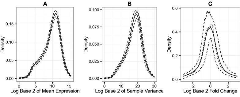
Kernel density estimates of the empirical distribution of sample test statistics for each gene for 200 SimSeq simulated RNA-seq datasets. The dotted line gives the estimate for the source dataset, the black line gives the average kernel density estimate over all simulations and the dashed lines give pointwise 0.025 and 0.975 quantiles of the kernel density estimates. The Gaussian kernel was used and the bandwidth was selected by Silverman’s rule of thumb. (A) The estimates for the log base 2 of mean expression level, (B) the estimates for the log base 2 of the sample variance and (C) the estimates for the log base 2 fold change

Figure 3 plots histograms of Spearman’s rank correlation for a fixed pair of genes involved in epithelial cell differentiation across 200 SimSeq simulated datasets and across 200 NB simulated datasets. For each simulated dataset, the computed value of Spearman’s rank correlation in the fixed gene pair was based on the set of normalized read counts [using TMM normalization (Robinson and Oshlack, 2010)]within each gene. The empirical distribution of Spearman’s rank correlation for the NB simulated datasets is centered at zero, whereas the empirical distribution is centered around the Spearman’s rank correlation value of 0.817 in the KIRC dataset. Figure 4 shows scatterplots of Spearman’s rank correlation for 28 genes involved in epithelial cell differentiation [GO:0030855 (Ashburner et al., 2000)] for one SimSeq simulated dataset versus the KIRC dataset and one NB simulated dataset versus the KIRC dataset. There is a strong positive linear trend for the SimSeq simulated data, whereas no trend is apparent for the NB simulated data.

Fig. 3.

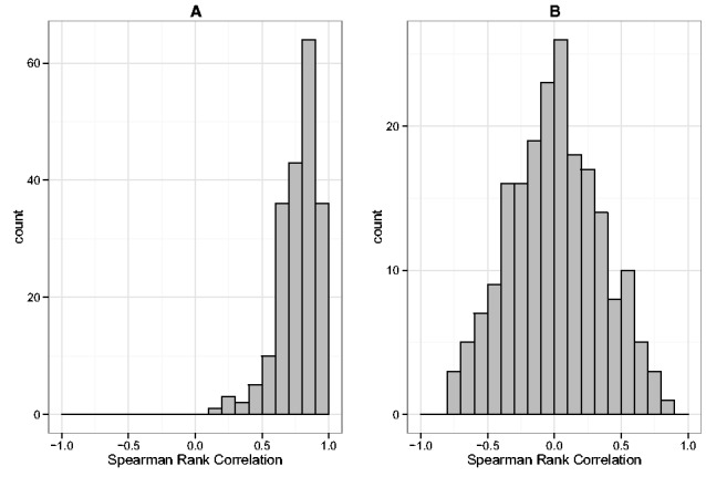
Distribution of Spearman’s rank correlation for a fixed pair of genes involved in epithelial cell differentiation [GO:0030855 (Ashburner et al., 2000)] over (A) 200 SimSeq simulated datasets and (B) 200 NB simulated datasets. For each simulated dataset, the computed value of Spearman’s rank correlation in the fixed gene pair was based on the set of normalized read counts [using TMM normalization (Robinson and Oshlack, 2010)] within each gene. Spearman’s rank correlation in the KIRC dataset was 0.817

Fig. 4.

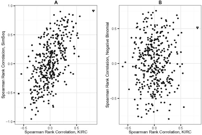
Scatterplot of Spearman’s rank correlation for 28 genes involved in epithelial cell differentiation [GO:0030855 (Ashburner et al., 2000)] for (A) one SimSeq simulated dataset versus the KIRC dataset and (B) one NB simulated dataset versus the KIRC dataset. Each point represents the Spearman’s rank correlation between a pair of genes based on the set of normalized read counts [using TMM normalization (Robinson and Oshlack, 2010)] within each gene. The triangular point highlights the fixed gene pair used in Figure 3

Figure 5 gives a smoothed kernel density estimate of the mean-variance relationship for the KIRC dataset, one NB simulated dataset and one SimSeq simulated dataset. The plot indicates that the mean-variance relationship of both of the simulated datasets matches that of the source dataset. Figure 6 gives a MA plot of the log base 2 fold change versus the log base 2 concentration [log counts per million or log CPM (Robinson et al., 2010)] for the KIRC dataset, one NB simulated dataset and one SimSeq simulated dataset. The empirical distribution of the log base 2 fold change of both simulated datasets exhibits variability similar to that of the source dataset.

Fig. 5.

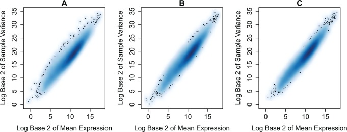
Mean-variance plots for (A) the KIRC dataset, (B) one SimSeq simulated dataset and (C) one NB simulated dataset. Each panel gives a smoothed kernel density estimate of the mean-variance relationship

Fig. 6.

MA plots for (A) the KIRC dataset, (B) one SimSeq simulated dataset and (C) one NB simulated dataset

5 Simulation study

We performed a parametric simulation study based on the NB model and compared results with a nonparametric simulation study using SimSeq. Rather than studying the entire corpus of statistical methods available for RNA-seq data, we instead elected to focus on several popular methods: DESeq2 (Anders and Huber, 2010; Love et al., 2014), edgeR (McCarthy et al., 2012; Robinson and Smyth, 2007, 2008; Robinson et al., 2010), QuasiSeq (Lund et al., 2012), Voom (Law et al., 2014) and SAMseq (Li and Tibshirani, 2013). We used the Wald test from the DESeq2 package (Anders and Huber, 2010; Love et al., 2014), the GLM likelihood ratio test from the edgeR package, the NegBinQLSpline method from the QuasiSeq package, the voom method from the limma package and the SAMseq method from the samr package. The following package versions were used: DESeq2 version 1.6.3, edgeR version 3.8.5, QuasiSeq version 1.0-4, limma version 3.22.1 and samr version 2.0. All default values of functions were used, except for the case of DESeq2, which we explain in further detail in Section 5.1.

5.1 Gene filtering criteria

A common practice in RNA-seq analysis is to exclude genes with average expression less than a particular threshold. Genes with low expression values tend to show little evidence of differential expression. By removing low count genes from the analysis, q values (Storey, 2002) for the remaining genes may decrease, allowing for more genes to be declared DE for a given multiple decision testing rule. Removing low count genes may also reduce the computational expense of subsequent analysis.

By default, DESeq2 applies two sets of filtering criteria (Love et al., 2014). The first set of criteria is known as automatic independent filtering. DESeq2 chooses a threshold for removal based on the value that will maximize the number of genes declared DE using a decision rule of estimated FDR (via Benjamini and Hochberg, 1995) less than 0.1. Because of computational stability of certain methods and to ensure comparability between the methods, we turned off the automatic independent gene filtering of the DESeq2 method and instead, applied a filtering rule where a given gene is included only if it has an average read count of at least 10 and at least two nonzero reads.

The second set of criteria DESeq2 uses is based on a Cook’s distance metric to flag outliers in the data. When sample size is between three and six, DESeq2 automatically removes genes with counts flagged as outliers, whereas for sample sizes of seven or more, DESeq2 replaces counts flagged as outliers with a trimmed mean over all samples in a given gene and treatment state, scaled by a normalization factor. We ran each simulation experiment twice, once with no Cook’s distance filtering and once with the DESeq2 Cook’s distance filtering rule prior to further analysis by each of the four methods.

5.2 Description of source dataset

We based our simulation experiments on the KIRC RNA-seq dataset from The Cancer Genome Atlas project (The Cancer Genome Atlas Research Network, 2013). The data were sequenced using the Illumina HiSeq 2000 RNA Sequencing Version 2 analysis platform and the estimated raw count for each gene was computed using RSEM software (Li and Dewey, 2011). The data are available for download from The Cancer Genome Atlas: https://tcga-data.nci.nih.gov/tcga/. The version of the KIRC dataset used was unc.edu_KIRC.IlluminaHiSeq_RNASeqV2.Level_3.1.5.0.

The KIRC dataset includes 72 pairs of matched columns with two samples from each individual affected with KIRC: one from a tumorous region of the body and one from a non-tumorous region. The dataset also contains additional columns of RNA-seq data from KIRC tumor and unmatched non-tumor samples. There was also one matched sample with a tumor type coded as an additional new primary type as opposed to the primary solid tumor type. For simplicity of design, we subsetted the data down to the paired data and omitted the additional new primary tumor type for a total of 72 pairs of matched columns of data over 20 531 genes.

5.3 Simulation experiments

In all our simulation experiments, 200 RNA-seq datasets were simulated to contain 5000 total genes with 4000 EE genes and 1000 DE genes. Genes in the simulated RNA-seq dataset that did not have an average read count of at least 10 and at least 2 nonzero reads were removed from the simulated matrix, and additional simulated genes were added, so that gene counts remained constant at 4000 EE genes and 1000 DE genes. We studied three different choices for the sample size within each treatment group: n = 5, n = 10 and n = 20. We ran each set of simulations twice, once using DESeq2’s Cook’s distance filtering and once without the filtering criteria.

5.3.1 Nonparametric simulation

We shaped the KIRC dataset into the form of the source dataset described in Section 2.1 and denote this dataset as Y. Let c be the vector of multiplicative normalization factors, which were computed by applying the TMM method to Y using the calcNormFactors function from the edgeR package. Let $\mathcal{G}$ be the set of all genes in Y.

For each simulated matrix of counts, the 1000 DE genes were selected by the default weighting scheme discussed in Section 3 and detailed as follows. Let $i=1,\dots ,72$ index pairs of columns in Y, and let $c_{i1}$ and $c_{i2}$ be the normalization factors for tumor and non-tumor columns for pair I, respectively. Then for each gene $g\in \mathcal{G}$, let $y_{gi1}$ and $y_{gi2}$ be the tumor and non-tumor counts for pair i, respectively, and let

$$d_{gi}=\log \left(\frac{y_{gi1}+1}{c_{i1}}\right)-\log \left(\frac{y_{gi2}+1}{c_{i2}}\right)\text{\hspace{0.17em}for\hspace{0.17em}}i=1,\dots ,72.$$

Apply a Wilcoxon Signed Rank test on the differences, $d_{g1},\dots ,d_{g72}$, to obtain a P value for testing the null hypothesis of no differential expression for each gene $g\in \mathcal{G}$. Given this set of P values, the local fdr is computed by the fdrtool package (Strimmer, 2008a, b). We then take one minus the local fdr for each gene to determine the weight vector w. We then applied the SimSeq algorithm for paired data (as described in Section 3) to obtain each simulated dataset.

5.3.2 NB simulation

We simulated counts from an NB distribution with parameters suggested by the KIRC dataset. For each $g\in \mathcal{G}$ we modeled y_git as $\text{NB}({\mu }_{git},{\omega }_{gt})$ for $i=1,\dots ,N_t$ and t = 1, 2, where $\text{E}(y_{git})={\mu }_{git}={\lambda }_{gt}{c}_{it}$ and $\text{Var}(y_{git})={\mu }_{git}+{\omega }_{gt}{\mu }_{git}^2$.

We estimated λ_gt based on the method of moments estimator ${\widehat{\lambda }}_{gt}=\frac{{\sum }_i{y}_{git}}{{\sum }_i{c}_{it}}$. Because we seek to simulate NB data with respect to two independent treatment groups, we estimated dispersions for each gene and treatment group in the following manner. For each gene $g\in \mathcal{G}$, let ${\widehat{\omega }}_{g1}$ be the tagwise estimate from the edgeR package using only the tumor treatment group data, rather than the paired data in the source dataset. Similarly, let ${\widehat{\omega }}_{g2}$ be the tagwise estimate using only the non-tumor treatment group data.

To reduce Monte Carlo variability between the nonparametric and parametric simulation procedures, we based the NB simulations on the same set of randomly selected EE and DE genes and the same set of randomly selected columns used in the nonparametric simulation algorithm. For a given simulated matrix, let ${\mathcal{G}}_0$ be the set of EE genes and ${\mathcal{G}}_1$ be the set of DE genes as randomly selected in its corresponding nonparametric simulated matrix and let ${\mathcal{G}}^{*}={\mathcal{G}}_0\cup {\mathcal{G}}_1$. Let $c_{11}^{*},\dots ,c_{1n}^{*}$ be the normalization factors from the tumor treatment columns used to simulate the treatment group 1 data and $c_{21}^{*},\dots ,c_{2n}^{*}$ be the normalization factors from the tumor columns used to simulate the treatment group 2 data in the nonparametric simulation algorithm.

We simulate the matrix X with entries x_git where $g\in {\mathcal{G}}^{*},i=1,\dots ,n$ and t = 1, 2 as follows. For each gene $g\in {\mathcal{G}}^{*}$, we simulate x_git from $\text{NB}({\lambda }_{gt}^{*}{c}_{it}^{*},{\omega }_{gt}^{*})$ where ${\lambda }_{gt}^{*}={\widehat{\lambda }}_{g1}$ and ${\omega }_{gt}^{*}={\widehat{\omega }}_{g1}$ if $g\in {\mathcal{G}}_0$ and ${\lambda }_{gt}^{*}={\widehat{\lambda }}_{gt}$ and ${\omega }_{gt}^{*}={\widehat{\omega }}_{gt}$ if $g\in {\mathcal{G}}_1$.

6 Simulation results

For each simulated matrix, the set of P values for each test of differential expression was converted to q values (Storey, 2002) in a manner equivalent to using the approach of Benjamini and Hochberg (1995) for FDR control. The estimated FDR is c for the multiple testing decision rule that rejects the null for the gth gene if and only if its q value is no larger than cutoff $c\in (0,1)$. The FDP at each cutoff was calculated as the number of type 1 errors divided by the total number of genes declared DE. The average FDP across replicate simulation runs provides empirical approximation of the true FDR for the q-value-based multiple testing decision rule.

6.1 Results without Cook’s filtering applied

Figure 7 shows average FDP minus q-value cutoff plotted against its corresponding q-value cutoff for each simulation algorithm (SimSeq or NB) and analysis method without using Cook’s distance in gene filtering. For the majority of statistical methods studied, the average FDP minus the target FDR level was greater for SimSeq than for the NB simulations. Using the voom method, average FDP minus the target FDR level was slightly lower for SimSeq than for the NB simulations at a sample size of 5 and showed little difference at a sample size of 10. Under the SAMseq method, which is a nonparametric method, there was little difference in terms of average FDP between the simulation methods at a sample size of 10. When sample size was increased to 20, the same trend as when sample size equaled 10 occurred.

Fig. 7.

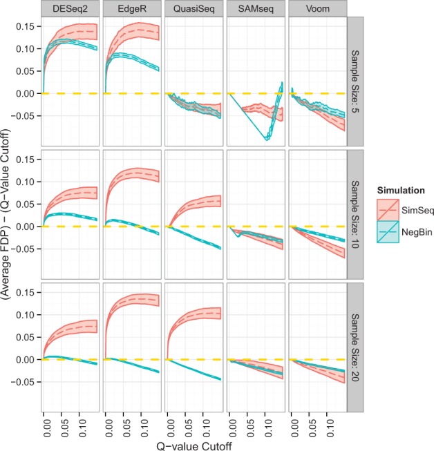
Plot of average FDP minus q-value cutoff for simulations without Cook’s distance filtering. The dashed golden line at 0 represents an average FDP that is exactly equal to its q-value cutoff, so that a method that achieves this parity is neither liberal nor conservative with respect to FDR control. The solid lines indicate approximate 95% pointwise confidence intervals for mean FDP minus q-value cutoff

Figure 8 contains boxplots of the 0.05 quantile of P values from null genes grouped by simulation type. Ideally, P values from null genes would be uniformly distributed on the interval (0, 1), so the 0.05 quantile of the null P values would be 0.05. For all of the parametric methods based on the NB distribution, the median 0.05 quantile of P values from null genes was lower than 0.05 under the SimSeq simulations. Furthermore, for the parametric analysis methods based on the NB distribution, the median 0.05 quantile of P values from null genes was lower when SimSeq was used to simulate data than when data were simulated according to NB distributions. In contrast, the median 0.05 quantile of P values from null genes was higher under the SimSeq simulations for the SAMseq and voom methods. This effect is consistent with average FDP minus the target FDR level being greater under the SimSeq simulations for parametric methods based on the NB distributions as smaller P values from null genes will tend to increase the proportion of type 1 errors given a multiple testing decision rule.

Fig. 8.

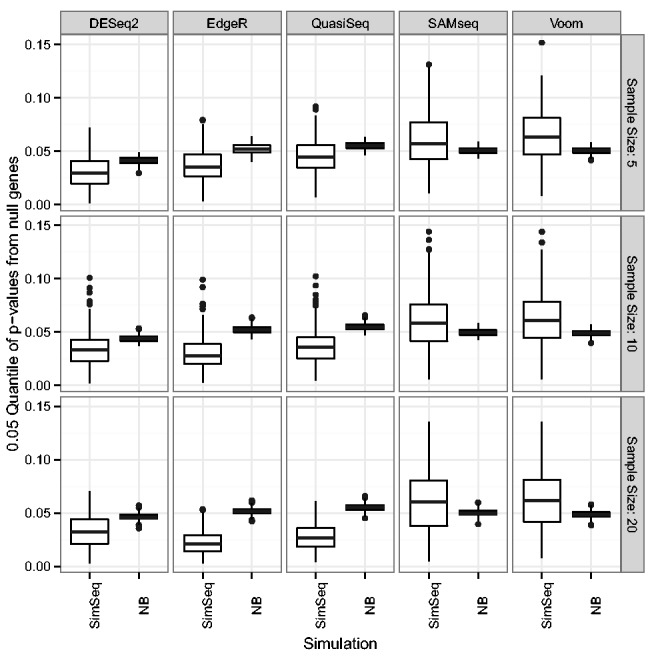
Boxplots of the 0.05 quantile of P values from null genes grouped by simulation type for simulations without Cook’s distance filtering applied

6.2 Results using Cook’s filtering

Figure 9 presents average FDP minus q-value cutoff plotted against its corresponding q-value cutoff for each simulation algorithm and analysis method with Cook’s distance filtering. At a sample size of 5, there were few differences in terms of FDR control between the two simulation procedures. When sample size was increased to the levels of 10 and 20, differences in FDR control between NB and SimSeq simulations were again apparent for the parametric analysis methods based on the NB distribution, although the differences tended to be somewhat reduced compared with the differences seen (in Fig. 7) without Cook’s distance filtering. Boxplots of the 0.05 quantile of P values from null genes (not shown) are similar to those in Figure 8 for the analysis without Cook’s distance filtering.

Fig. 9.

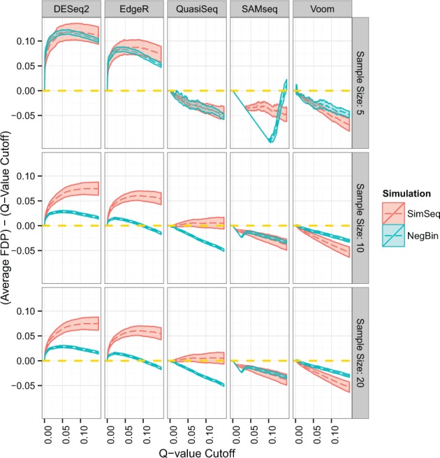
Plot of average FDP minus q-value cutoff for simulations with Cook’s distance filtering. The dashed golden line at 0 represents an average FDP that is exactly equal to its q-value cutoff, so that a method that achieves this parity is neither liberal nor conservative with respect to FDR control. The solid lines indicate approximate 95% pointwise confidence intervals for mean FDP minus q-value cutoff

6.3 Simulating from a more homogeneous source dataset

We repeated the simulation experiments described in Section 5.3 with a sample size of three using a dataset from Bottomly et al. (2011) as the source RNA-seq dataset. The Bottomly et al. dataset contains two genotypes of genetically identical mice with sample sizes of 10 and 11 in the two genotype groups, which is in contrast to the KIRC dataset that involves subjects from heterogeneous human populations. Plots of average FDP minus target FDR level with and without Cook’s distance filtering are provided in Figures 1 and 2 of the Supplementary Files. In general, the differences in the point estimates of average FDP minus target FDR level between the SimSeq simulations and the NB simulations were smaller than observed in the results from the KIRC dataset analysis. This suggests that the NB assumption for gene-specific marginal read count distributions may be more reasonable for data from genetically identical experimental units than it is for more heterogeneous experimental units. Although the point estimates of the discrepancy between average FDP and target FDR were similar between the SimSeq and NB simulations, variation in FDP remained much higher for SimSeq simulation than NB simulation despite the greater homogeneity in experimental units.

7 Discussion

The principal differences between the SimSeq algorithm for simulating RNA-seq data and the NB simulations are that the SimSeq algorithm makes no parametric distributional assumptions and preserves the complex gene dependence structure of the original dataset. In contrast, the NB method simulates data for each gene independently according to marginal NB distributions. Thus, we should expect methods that are more robust to varying distributional assumptions to behave more similarly between the two simulation methods. Conversely, methods that are less robust to departures from the parametric distributional assumptions on which they are based should perform worse when applied to the SimSeq simulated data. Under the SAMseq and Voom methods, which are not based on NB assumptions, there is little difference between the two simulation types in terms of average FDP. In contrast, we see substantial differences in FDR control properties across simulation types for the other analysis methods that rely on NB assumptions.

The difference in the results between the two simulation approaches in terms of FDR control is important to point out. Some methods that appeared to control FDR or were slightly liberal with respect to FDR control under the NB simulations failed to control FDR under the SimSeq simulations. Further, the ranking of each of the methods in terms of FDR control sometimes differed depending on whether NB or the SimSeq simulation was used.

It is also worth discussing the liberalness of the DESeq2 and edgeR methods in general. Although other simulation studies have already indicated that both of these methods exhibit liberalness in FDR control (Burden et al., 2014; Soneson and Delorenzi, 2013), our simulation study shows even greater discrepancies between nominal and actual FDR control when these methods are applied to datasets simulated by SimSeq from the heterogeneous KIRC dataset. When we repeated the simulation study using the Bottomly et al. dataset as the source dataset (for which the NB assumption may be more reasonable), the liberalness of the two methods decreased, although both methods still remained liberal.

Using the additional Cook’s distance filtering criteria as implemented in the DESeq2 package reduced the difference in average FDP between the nonparametric and parametric simulation procedures. The nonparametric SimSeq algorithm is capable of sampling extreme values that lie in the source dataset that are unlikely to be generated by a parametric simulation algorithm. The presence of such extreme values in SimSeq-generated data (that are not subjected to Cook’s distance filtering) may partly explain the high average FDP values for the fully parametric analysis methods. Differences in FDR control across simulation strategies that remain after Cook’s distance filtering show the effect of gene dependence and departures of empirical data from NB distributions that cannot be easily corrected by outlier removal.

One of the most striking features of Figures 2–4 (and Supplementary Figs. S1 and S2) is the larger variation in simulation results for SimSeq compared with the NB simulation method. This larger variation is a consequence of the realistic dependence from gene to gene in data simulated by SimSeq. Dependence among genes leads to dependence among P values within each analysis. This dependence among P values leads to greater variation in quantities computed from P values, such as estimates of FDR and sample quantiles of the P values from null genes. Results from NB simulations with independent genes may lead researchers to underestimate the uncertainty in simulation-based estimates of FDR. SimSeq creates a less optimistic but more accurate picture of the uncertainty that can be expected when analysis methods are applied to real RNA-seq data.

We also compared the performance of the four statistical methods using partial area under the receiver operating characteristic curve (PAUROCC). PAUROCC indicates how well an analysis method rank orders genes from most significant to least significant. The specific value of PAUROCC utilized was calculated as the area under the receiver operating characteristic curve for specificity values ≥0.95. These specificity values correspond to type I error rates no larger than 0.05. PAUROCC was neither systematically higher nor systematically lower under the NB simulations over the class of statistical analysis methods studied.

A factor to consider when using the SimSeq package is the choice of the source dataset. The source datasets used in this article were the KIRC dataset from the Cancer Genome Atlas project and the Bottomly et al. dataset. For the KIRC dataset, the samples stem from a heterogeneous population crossing diverse factors such as race, gender, age and ethnicity. This is in contrast to the Bottomly et al. dataset that contains homogeneous samples with genetically identical mice. The simulation experiments of Section 6 indicate that there are larger differences in average FDP minus target FDR level between the SimSeq simulations and the NB simulations for our source datasets based on a heterogeneous population than for the source dataset based on a more homogeneous population. To investigate the performance of analysis methods on relatively homogeneous observational or experimental units, more homogeneous source datasets should be used. As more large RNA-seq datasets become publicly available, the number and variety of source dataset options will increase.

In conclusion, important performance benchmarks such as average FDP relative to nominal FDR can change drastically between the two simulation procedures depending on the statistical method used. The SimSeq algorithm simulates RNA-seq data that closely matches the marginal distributions and complex dependence structure of real RNA-seq data. Simulation studies using this method more accurately reflect average FDPs likely to be obtained in practice. Simulation experiments that rely on parametric models may paint an overly optimistic picture for the efficacy of a given method. As such, in evaluating current and future statistical methodologies in gene expression analysis, we recommend using the SimSeq algorithm because it more closely matches the complex structure of RNA-seq data.

Funding

This work was supported by the National Science Foundation [grant numbers IOS0922746, IOS1339348 and DMS1313224] and by the National Institute of General Medical Science (NIGMS) of the National Institutes of Health and the joint National Science Foundation/NIGMS Mathematical Biology Program [grant number R01GM109458].

Conflict of interest: none declared.

References

- Anders S., Huber W. (2010) Differential expression analysis for sequence count data. Genome Biol. , 11, R106. [DOI] [PMC free article] [PubMed] [Google Scholar]
- Ashburner M., et al. (2000) Gene ontology: tool for the unification of biology. Nat. Genet. , 25, 25–29. [DOI] [PMC free article] [PubMed] [Google Scholar]
- Benjamini Y., Hochberg Y. (1995) Controlling the false discovery rate: a practical and powerful approach to multiple testing. J. R. Stat. Soc. B , 57, 289–300. [Google Scholar]
- Bottomly D., et al. (2011) Evaluating gene expression in c57bl/6j and dba/2j mouse striatum using rna-seq and microarrays. PLoS One , 6, e17820. [DOI] [PMC free article] [PubMed] [Google Scholar]
- Bullard J., et al. (2010) Evaluation of statistical methods for normalization and differential expression in mRNA-Seq experiments. BMC Bioinformatics , 11, 94. [DOI] [PMC free article] [PubMed] [Google Scholar]
- Burden C., et al. (2014) Error estimates for the analysis of differential expression from RNA-seq count data. Peer J. 2, e576. [DOI] [PMC free article] [PubMed] [Google Scholar]
- Dillies M.-A., et al. (2013) A comprehensive evaluation of normalization methods for Illumina high-throughput RNA sequencing data analysis. Brief. Bioinform ., 14, 671–683. [DOI] [PubMed] [Google Scholar]
- Gadbury G.L., et al. (2008) Evaluating statistical methods using plasmode data sets in the age of massive public databases: an illustration using false discovery rates. PLoS Genet. , 4, e1000098. [DOI] [PMC free article] [PubMed] [Google Scholar]
- Griebel T., et al. (2012) Modelling and simulating generic RNA-Seq experiments with the flux simulator. Nucleic Acids Res. , 40, 10073–10083. [DOI] [PMC free article] [PubMed] [Google Scholar]
- Law C.W., et al. (2014) Voom: precision weights unlock linear model analysis tools for RNA-seq read counts. Genome Biol. , 15, R29. [DOI] [PMC free article] [PubMed] [Google Scholar]
- Li B., Dewey C. (2011) RSEM: accurate transcript quantification from RNA-Seq data with or without a reference genome. BMC Bioinformatics , 12, 323. [DOI] [PMC free article] [PubMed] [Google Scholar]
- Li J., Tibshirani R. (2013) Finding consistent patterns: a nonparametric approach for identifying differential expression in RNA-Seq data. Stat. Methods Med. Res. , 22, 519–536. [DOI] [PMC free article] [PubMed] [Google Scholar]
- Liang K., Nettleton D. (2010) A hidden Markov model approach to testing multiple hypotheses on a tree-transformed gene ontology graph. J. Am. Stat. Assoc. , 105, 1444–1454. [Google Scholar]
- Love M.I., et al. (2014) Moderated estimation of fold change and dispersion for RNA-Seq data with DESeq2. Genome Biol. , 15, 550. [DOI] [PMC free article] [PubMed] [Google Scholar]
- Lund S., et al. (2012) Detecting differential expression in RNA-sequence data using quasi-likelihood with shrunken dispersion estimates. Stat. Appl. Genet. Mol. Biol. , 11, 8. [DOI] [PubMed] [Google Scholar]
- McCarthy D.J., et al. (2012) Differential expression analysis of multifactor RNA-Seq experiments with respect to biological variation. Nucleic Acids Res. , 40, 4288–4297. [DOI] [PMC free article] [PubMed] [Google Scholar]
- Nettleton D., et al. (2008) Identification of differentially expressed gene categories in microarray studies using nonparametric multivariate analysis. Bioinformatics , 24, 192–201. [DOI] [PubMed] [Google Scholar]
- Reeb P.D., Steibel J.P. (2013) Evaluating statistical analysis models for RNA sequencing experiments. Front. Genet. , 4, 178. [DOI] [PMC free article] [PubMed] [Google Scholar]
- Robinson D.G., Storey J.D. (2014) subSeq: Determining appropriate sequencing depth through efficient read subsampling. Bioinformatics , 30, 3424–3426. [DOI] [PMC free article] [PubMed] [Google Scholar]
- Robinson M.D., Oshlack A. (2010) A scaling normalization method for differential expression analysis of RNA-seq data. Genome Biol. , 11, R25. [DOI] [PMC free article] [PubMed] [Google Scholar]
- Robinson M.D., Smyth G.K. (2007) Moderated statistical tests for assessing differences in tag abundance. Bioinformatics , 23, 2881–2887. [DOI] [PubMed] [Google Scholar]
- Robinson M.D., Smyth G.K. (2008) Small-sample estimation of negative binomial dispersion, with applications to SAGE data. Biostatistics , 9, 321–332. [DOI] [PubMed] [Google Scholar]
- Robinson M.D., et al. (2010) edgeR: a Bioconductor package for differential expression analysis of digital gene expression data. Bioinformatics , 26, 139–140. [DOI] [PMC free article] [PubMed] [Google Scholar]
- Soneson C., Delorenzi M. (2013) A comparison of methods for differential expression analysis of RNA-seq data. BMC Bioinformatics , 14, 91. [DOI] [PMC free article] [PubMed] [Google Scholar]
- Storey J.D. (2002) A direct approach to false discovery rates. J. R. Stat. Soc. B , 64, 479–498. [Google Scholar]
- Strimmer K. (2008a) fdrtool: a versatile R package for estimating local and tail area-based false discovery rates. Bioinformatics , 24, 1461–1462. [DOI] [PubMed] [Google Scholar]
- Strimmer K. (2008b) A unified approach to false discovery rate estimation. BMC Bioinformatics , 9, 303. [DOI] [PMC free article] [PubMed] [Google Scholar]
- The Cancer Genome Atlas Research Network (2013) Comprehensive molecular characterization of clear cell renal cell carcinoma. Nature , 499, 43–49. [DOI] [PMC free article] [PubMed] [Google Scholar]
Associated Data
This section collects any data citations, data availability statements, or supplementary materials included in this article.