

Abstract
Trapping and preconcentrating particles and cells for enhanced detection and analysis are often essential in many chemical and biological applications. Existing methods for diamagnetic particle trapping require the placement of one or multiple pairs of magnets nearby the particle flowing channel. The strong attractive or repulsive force between the magnets makes it difficult to align and place them close enough to the channel, which not only complicates the device fabrication but also restricts the particle trapping performance. This work demonstrates for the first time the use of a single permanent magnet to simultaneously trap diamagnetic and magnetic particles in ferrofluid flows through a T-shaped microchannel. The two types of particles are preconcentrated to distinct locations of the T-junction due to the induced negative and positive magnetophoretic motions, respectively. Moreover, they can be sequentially released from their respective trapping spots by simply increasing the ferrofluid flow rate. In addition, a three-dimensional numerical model is developed, which predicts with a reasonable agreement the trajectories of diamagnetic and magnetic particles as well as the buildup of ferrofluid nanoparticles.
I. INTRODUCTION
A variety of microfluidic techniques have been developed to trap and preconcentrate particles for enhanced capturing and binding of analyte molecules as well as enhanced detection, etc.1–4 Particles can be immobilized onto solid surfaces through direct contact via either mechanical filters or chemical coatings, which is, however, prone to irreversible adhesions with a potentially high probability of device fouling.5,6 More preferably, particles can be captured in a flowing suspension through the use of an external force, where the accumulated particles can be readily dispersed by either lowering (or switching off) the force field or increasing the flow rate.2–4 A number of non-magnetic force fields,1,7 including acoustic,8,9 electric,10–13 and optical14–16 forces, have been demonstrated to enrich various types of particles and cells in microfluidic devices. Compared to these contactless methods, magnetic trapping of particles has several advantages such as low cost, heating free (except for electromagnets), and near independence of the suspending medium properties (e.g., ionic concentration and pH value).17–19
Magnetic trapping relies on the magnetophoretic motion of particles induced in a non-uniform magnetic field,20–22 which has been reported for both magnetic (including paramagnetic) and diamagnetic (or simply speaking, nonmagnetic) particles. Magnetic (either intrinsic or extrinsic) particles are pulled along magnetic field gradients toward the magnetic source in diamagnetic (e.g., water) or less magnetic media.23,24 This positive magnetophoretic motion has been widely utilized to concentrate and isolate magnetically-tagged target cells (e.g., circulating tumor cells) from a heterogeneous mixture.25–27 Diamagnetic particles must be re-suspended in magnetic media like ferrofluids28–33 and paramagnetic solutions,34,35 so that they experience negative magnetophoresis and are repelled away from the magnetic source.36–42 While magnetic particle trapping has been demonstrated with single magnets placed on one side of the particle flowing microchannel,23–27 diamagnetic particle trapping can only take place stably with one or multiple pair(s) of magnets arranged on both sides of the channel.43–47 The strong attractive or repulsive force between the pair(s) of magnets often renders it difficult to align the magnets and place them close enough to the particle flowing channel. This not only complicates the device fabrication but also restricts the particle trapping performance due to the limited magnetic fields and magnetic field gradients inside the microchannel.
In this work, we demonstrate for the first time the use of a single permanent magnet to continuously trap and preconcentrate diamagnetic particles in ferrofluid flows through a T-shaped microchannel. Moreover, magnetic particles can be simultaneously trapped while to a different location of the same microchannel via the same magnet. Such an ability of trapping two (or even more) types of particles in the same device makes it possible to carry out simultaneous bioassays of several sample components. A few works have been reported in this direction, where magnetic particles bearing different surface functioning are trapped to form two or more plugs.48,49 Recently, Pamme's group50 has demonstrated the application of diamagnetic repulsion and magnetic attraction forces for the simultaneous trapping of diamagnetic and magnetic particles, respectively, in a paramagnetic solution (MnCl2) using a single set of magnets. However, a magnet assembly was still needed in order to hold and align a pair of attracting magnets on the two sides of a capillary.
To understand the dissimilar trapping processes for diamagnetic and magnetic particles in ferrofluid microflows, we also develop in this work a three dimensional (3D) numerical model to track the particle trajectories in the T-shaped microchannel. Moreover, the redistribution of ferrofluid nanoparticles (i.e., the magnetic nanoparticles that contribute to the magnetization of ferrofluids)29–31,46,51 is simulated by solving the ferrofluid concentration field under the application of a combined magnetic and hydrodynamic field. The numerical predictions are compared with the experimentally obtained particle and ferrofluid images at three different flow rates for which the diamagnetic and magnetic particles are simultaneously trapped and sequentially released, respectively.
II. EXPERIMENTATION
A. Microfluidic chip fabrication
Fig. 1 shows a picture of the microfluidic chip used in experiments, which was fabricated with polydimethylsiloxane (PDMS) using a custom-modified soft lithography method as presented in our earlier work.38 The 60 μm deep T-shaped microchannel is composed of a 200 μm wide, 10 mm long main-branch and two 100 μm wide, 8 mm long side-branches. A 1/8″ × 1/8″ × 1/16″ (thick) Neodymium-Iron-Boron permanent magnet (B222, K&J Magnets, Inc.) was embedded into PDMS and placed right behind the T-junction with an edge-to-edge distance of 450 μm. The magnet was designed to be symmetrically located about the centerline of the main-branch, which was very difficult (if not impossible) to implement under the microscope (Eclipse TE2000U, Nikon Instruments). Such a condition was, however, found unnecessary through experiment and simulation because the dimension of the magnet is much larger than that of the microchannel and the magnetic field distribution within the channel region remains nearly unchanged for small off-center distances. The magnet is in direct contact with the glass slide, i.e., the bottom surface of the magnet is at the same plane as the bottom wall of the microchannel. Its magnetization direction (through the thickness) is parallel to the ferrofluid flow direction (see the block arrow in Fig. 1) in the main-branch of the microchannel.
FIG. 1.

Picture of the PDMS-based microfluidic chip (the microchannel and reservoirs are filled with green food dye for clarity) used in experiments. The block arrows indicate the ferrofluid flow directions in the T-shaped microchannel. A permanent magnet is embedded into the PDMS and placed behind the T-junction of the microchannel nearly symmetrically with respect to the centerline of the main-branch.
B. Particle solution preparation and experimental method
The base solution used in our experiments is a water-based ferrofluid, EMG 408 from Ferrotec Corp., which is a black-brown liquid consisting of 1.2% (in volume) 10 nm-diameter sub-domain magnetic nanoparticles. By adding deionized (DI) water (Fisher Scientific), we first diluted the ferrofluid to 0.05× the original concentration by volume. Then, 2.85 μm-diameter magnetic particles (with a standard deviation of 0.105 μm, Bangs Laboratories, Inc.) and 9.9 μm-diameter diamagnetic polystyrene particles (with a non-uniformity of smaller than 5%, Thermo Fisher Scientific) were mixed and re-suspended into the 0.05× ferrofluid at a final concentration of around 106 particles per ml each. Also, 0.5% (in volume) Tween 20 (Fisher Scientific) was added to the suspension for the purpose of reducing particle aggregations and adhesions to microchannel walls. Prior to uses, the particle solution was stirred using a fixed speed vortex mixer (Fisher Scientific) for a uniform dispersion. It was driven to flow through the T-shaped microchannel by an infusion syringe pump (KD Scientific). The movements and trapping of diamagnetic and magnetic particles were visualized at the T-junction of the microchannel using an inverted microscope (Eclipse TE2000U, Nikon Instruments) and recorded with a CCD camera (Nikon DS-Qi1Mc) at a rate of about 15 frames/s. The effects of flow rate on ferrofluid concentration field at the T-junction were also investigated in the absence of both types of particles. The captured videos and images were post-processed through the Nikon imaging software (NIS-Elements AR 2.30).
III. SIMULATION
A 3D numerical model was developed to predict and understand the magnetic trapping of diamagnetic and magnetic particles in ferrofluid flow through the T-shaped microchannel. This model considers only the one-way actions that the flow and magnetic fields have on the suspended two types of particles and as well the ferrofluid nanoparticles. The dynamic actions of these particles on the flow and magnetic fields are, however, neglected in order to simplify the model. Also neglected are the dipole-dipole interactions among the same type or different types of particles in a magnetic field. Such a treatment of particle-fluid and particle-particle interactions has been demonstrated reasonable in previous theoretical studies from the groups of Mao et al.,28,32,37,40,42 Nguyen et al.,41 and Xuan et al.30,31,33,36,39 as long as the particle and ferrofluid concentrations are both low. These conditions are fulfilled in the current work because of the use of a dilute particle suspension in a diluted ferrofluid. Specifically, the magnetic susceptibility of 0.05× EMG 408 was calculated to be only 0.025.52 This small value is not expected to significantly affect the flow and magnetic fields unless the ferrofluid is strongly accumulated near the permanent magnet. It is, however, important to note that the current model can only predict the onset of particle trapping, not the trapping process during which the accumulation of diamagnetic and/or magnetic particles will affect the flow and magnetic fields.47
A. Governing equations
1. Flow field and concentration field of the ferrofluid
Since the dynamic influences of the suspended microparticles (both diamagnetic and magnetic) and nanoparticles (magnetic) on the flow and magnetic fields are all neglected in our model, the ferrofluid is assumed to behave like water with homogeneous properties under the application of a magnetic field.28–33,36–41,47 As such, the steady-state flow field in the T-shaped microchannel, , is governed by the conventional continuity and Navier-Stokes equations
| (1) |
| (2) |
where , , and are the ferrofluid density, pressure, and viscosity, respectively. The actions of the flow and magnetic fields on each magnetic nanoparticle generate a positive magnetophoretic motion, (Ref. 53)
| (3) |
| (4) |
| (5) |
In the above, is the permeability of the free space, is the nominal diameter of the magnetic nanoparticle with a magnetization of , is the magnetic field with being the magnitude, is the saturation moment of the magnetic nanoparticle with being the magnitude, is the Boltzmann constant, and is the ferrofluid temperature. This migration toward the magnet (specifically the center of the magnet at which the magnetic field strength is the highest) results in a redistribution of the magnetic nanoparticles and hence a non-uniform ferrofluid concentration, , which is governed by the following convection-diffusion equation:
| (6) |
where the diffusion coefficient can be estimated from the Stokes-Einstein equation, .
2. Transport of diamagnetic and magnetic microparticles
The trajectory of a magnetic or diamagnetic particle in the ferrofluid microflow under a magnetic field is determined by its velocity, ,
| (7) |
where and are the particle velocities due to the magnetophoretic (from the magnetic field) and gravity-buoyancy (from the ferrofluid) actions, respectively, and each expressed as36
| (8) |
| (9) |
In the above, a, , and are the radius, mass density, and magnetic susceptibility of the particle (either magnetic or diamagnetic) to be trapped, is the drag coefficient that accounts for the wall retardation effects, is the gravitational acceleration, and
| (10) |
is the ferrofluid magnetization.53 Two expressions of are used for particle motions parallel and normal to the top/bottom walls of the microchannel, respectively,36
| (11) |
| (12) |
where is the smaller distance between the particle center and the top and bottom walls of the microchannel, respectively.
3. Magnetic field
In the absence of the particle and ferrofluid effects, the magnetic field generated by a rectangular permanent magnet can be described by Furlani's analytical formulae.54 Thus, the large air box around the magnet (typically 10-time size of the latter55) is no longer needed in the computational domain, which can dramatically reduce the computational time. The approach that we used the analytical formulae (skipped here for brevity) to compute the magnetic field components in the three directions will be presented in Section III C.
B. Computational domain and boundary conditions
The magnetic/diamagnetic particle trapping and ferrofluid concentration variation both take place in the T-junction region of the microchannel. Therefore, a 3D computational domain of the T-junction is set up as shown in Fig. 2, which considers only a length of 1000 μm in the main-branch and 500 μm in each side-branch to reduce the computational cost. Note that one half of the domain in Fig. 2 is actually sufficient for the numerical model if the magnet is located symmetrically with respect to the microchannel. However, we still used the full domain in Fig. 2 in our model for the purpose of accommodating any offer-center displacement of the magnet. The following boundary conditions were prescribed:
FIG. 2.

Isometric view of the 3D computational domain of the T-junction with dimensions being labeled. The insets Ι and II show the enlarged view of the meshes at the inlet region of the main-branch and the outlet region of one side-branch, where the boundary layers near the channel walls are highlighted.
Inlet: imposed volume flow rate; with being the bulk concentration of 0.05× EMG 408 ferrofluid far away from the magnet.
Two outlets: zero shear stress and ; with n denoting the unit normal vector of a surface.
All channel walls: no slip with ; no penetration with where denotes the concentration flux.
C. Numerical method
The diamagnetic and magnetic particle trapping in ferrofluid flow through the T-shaped microchannel in Fig. 1 were simulated in COMSOL® 4.3b over the 3D computational domain in Fig. 2. The Laminar Flow module was used to solve for the ferrofluid flow field from Eqs. (1) and (2). The Transport of Diluted Species module was used to solve for the ferrofluid concentration field from Eq. (6). Note that these two fields were not coupled under the assumptions made above and hence were solved separately in our model. The 3D magnetic field of the rectangular permanent magnet was determined directly from Furlani's analytical formulae54 that were input to COMSOL as variables. The center of the magnet was specified as the origin of the Cartesian coordinates in our model such that the coordinate conversion of these formulae was avoided. The magnetic field gradients were calculated using the built-in mathematical functions in COMSOL. As an example, Fig. 3 shows the magnetic field contour (see the background color) and vectors (see the arrows) inside the T-shaped microchannel. The magnetic field is high in the two side-branches and decays in the main-branch with distance away from the magnet. Moreover, the vectors of magnetic field are obliquely downward (see the inset in Fig. 3) because the top channel wall is nearer to the center of the magnet and hence has a stronger magnetic field than the bottom one.
FIG. 3.

Magnetic field contour (indicated by the color map) and vectors (indicated by the arrows) inside the T-shaped microchannel with the inset being a zoom-in view of the corner region.
The Streamline function in COMSOL was used to trace the diamagnetic and magnetic particle motions in ferrofluid flows at the T-junction via Eq. (7). To overcome the intrinsic issue of streamline stopping at the channel walls due to the non-zero magnetophoretic particle velocity in the normal direction, we used the built-in operator functions in COMSOL to track the particle-wall distance. Once a (magnetic or diamagnetic) particle was confirmed to reach a wall, the normal component of the magnetophoretic velocity was set to zero while the tangential component remained unvaried. This step requires that the mesh size near the wall be less than the particle radius. Therefore, fine boundary layer meshes were used on each of the four channel walls, as highlighted in the insets I and II in Fig. 2. Note also that the mesh in the bulk of the side-branches (see inset II) was finer than that in the bulk of the main-branch (see inset I), which was designed for accurately computing the highly non-uniform concentration field in the former. Moreover, to overcome the false numerical diffusion, we assumed a correction coefficient of 6 for the magnetophoretic velocity of ferrofluid nanoparticles, i.e., in Eq. (3), as was done previously.56 This value was selected by obtaining a visually (i.e., qualitatively) strong variation in the ferrofluid concentration contour while the predicted maximum concentration is still relatively low to ensure the validity of a dilute ferrofluid. A nonlinear iterative solver was used to solve the model, which was performed in the Palmetto Cluster at Clemson University. A grid independence study was conducted, from which a (maximum) mesh size of 6 μm was found to be sufficient for the ferrofluid velocity and concentration simulation. The values of the physical properties and geometrical parameters are summarized in Table I.
TABLE I.
Physical properties and geometric parameters used in the numerical simulation.
| Component | Symbol | Description | Value |
|---|---|---|---|
| Magnet | Residual magnetization | A/m | |
| Thickness | 1.588 mm | ||
| Length | 3.176 mm | ||
| Height | 3.176 mm | ||
| Magnet-channel distance | 0.45 mm | ||
| Ferrofluid | d | Diameter of magnetic nanoparticles | 10 nm |
| Bulk ferrofluid concentration (0.05× EMG 408) | 0.06% | ||
| Saturation moment of magnetic nanoparticles | |||
| Dynamic viscosity of the ferrofluid | |||
| mass density of the ferrofluid | 1070 kg/m3 | ||
| Particles | 2a | Diameter of magnetic microparticles | 2.85 μm |
| Diameter of diamagnetic microparticles | 9.9 μm | ||
| Magnetic particle susceptibility | 0.024 | ||
| Diamagnetic particle susceptibility | 0 | ||
| Density of magnetic particles | 1230 kg/m3 | ||
| Density of diamagnetic particles | 1050 kg/m3 |
IV. RESULTS AND DISCUSSION
A. Experimental implementation of diamagnetic and magnetic particle trapping
The top-view snapshot images in Fig. 4 show the time development for the simultaneous trapping of 9.9 μm-diameter diamagnetic particles and 2.85 μm-diameter magnetic particles in ferrofluid flow through the T-shaped microchannel. The volumetric flow rate is 55 (±5) μl/h in the main-branch with an average flow velocity of 1.27 mm/s, beyond which diamagnetic particles can no longer be completely trapped. Diamagnetic particles experience negative magnetophoresis in ferrofluids and tend to move away from the magnet. They thus get trapped in the main-branch before entering the two side-branches due to the counterbalance of the pressure-driven flow therein. Moreover, they form a V-shaped pattern, where, as highlighted by the curved block arrows in Fig. 4 (middle), the trapped particles in each arm slowly circulate upstream from near the sidewall to the channel center and then downstream toward the T-junction. This happens as the magnetophoretic particle velocity is nearly uniform across the width of the main-branch (which is very small compared to the dimension of the magnet), while the pressure-driven ferrofluid flow has a parabolic velocity profile.46,47 In addition, the V-shaped trapping zone in Fig. 4 (right) extends upstream as more diamagnetic particles are trapped. However, the intersection point of the two arms seems to remain nearly unchanged throughout the trapping process. The slight asymmetry of the particle trapping zone in Fig. 4 (right) may be because the magnet is not perfectly symmetric about the main-branch.
FIG. 4.

Time (labeled on the images) development for simultaneous trapping of 9.9 μm-diameter diamagnetic particles and 2.85 μm-diameter magnetic particles in 0.05 × EMG 408 ferrofluid flow through a T-shaped microchannel at a volume flow rate of 55 μl/h. The straight block arrows on the left image indicate the flow directions. The curved block arrows on the middle image highlight the circulating directions of the trapped diamagnetic particles.
In contrast, magnetic particles experience positive magnetophoresis in ferrofluids and hence get trapped onto the back wall of the T-junction that faces the magnet. Moreover, due to the magnetic field gradients in the depth direction of the microchannel (see Fig. 3), magnetic particles are actually concentrated onto the top corner region. This latter position is opposite to that of diamagnetic particles which should be trapped onto the bottom surface of the main-branch. Therefore, magnetic particles are not clearly visible in Fig. 4 as they are in a different focal plane than diamagnetic particles and also much smaller than the latter. This is evidenced from the snapshot images in Fig. 5, which are taken when the focal plane of the microscope objective is on diamagnetic particles (right, near the bottom channel wall) and magnetic particles (left, near the top channel wall), respectively. The ferrofluid flow tends to sweep the trapped magnetic particles and carry them to the downstream if the flow inertia is sufficiently strong. This action produces a convex shape of the magnetic particle trapping zone as demonstrated by the left image in Fig. 5. This trapping zone overlaps with that of ferrofluid nanoparticles, which cannot be visually identified in Fig. 5. We therefore conducted a pure ferrofluid flow experiment through the T-shaped microchannel at the same flow rate as in Figs. 4 and 5. The result will be shown in Fig. 7 and explained along with the numerical prediction in Section IV B.
FIG. 5.

Top-view snapshot images of simultaneous diamagnetic and magnetic particle trapping at the T-junction region when the focal plane of the microscope objective is near the bottom (right, diamagnetic particles are in focus) and the top (left, magnetic particles are in focus) walls of the microchannel, respectively. Other conditions are referred to in the caption of Fig. 4.
FIG. 7.

Comparison of top-view experimental images (left column) and numerical predictions (right column) for simultaneous diamagnetic/magnetic particle trapping (a) and ferrofluid nanoparticle buildup ((b), in the absence of microparticles) at the T-junction region of the microchannel. The focal plane of the microscope objective is in the middle of the channel depth. The volume flow rate is 55 μl/h in the experiment and 40 μl/h in the simulation. Note that the bulk ferrofluid concentration far away from the magnet is 0.05 × 1.2%. The block arrows in (b) indicate the flow directions.
B. Numerical simulation of diamagnetic and magnetic particle trapping
The experimentally demonstrated simultaneous trapping of diamagnetic and magnetic particles in ferrofluid flow can be understood by the simulated 3D particle trajectories at the T-junction region in Fig. 6(a). Multiple particles, which are evenly distributed over the channel cross-section, are released at the inlet of the main-branch. Diamagnetic particles (red lines) are predicted to travel toward the bottom channel wall of the main-branch due to negative magnetophoresis (see also Fig. 3) and get trapped before entering the side-branches. In contrast, magnetic particles (green lines) are predicted to quickly migrate toward the top channel wall due to positive magnetophoresis (see also Fig. 3) and get trapped onto the top edge of the back wall at the T-junction. These predictions are consistent with the experimental observations in Figs. 4 and 5. However, our model is unable to simulate the circulation of the trapped diamagnetic particles. Moreover, the maximum volume flow rate for the simultaneous diamagnetic and magnetic particle trapping is predicted to be only 40 μl/h, which is about 25% less than the experimentally measured value. These deviations may be due to the neglect of particle and ferrofluid effects on magnetic and flow fields in the current model. The ferrofluid effects can be viewed from its concentration contour over a series of cross-sectional slices along the main-branch in Fig. 6(b). The ferrofluid becomes increasingly non-uniform on approaching the T-junction, where magnetic nanoparticles are more significantly concentrated near the top channel wall due to their positive magnetophoretic motion. These gradients can cause disturbances to the magnetic and flow fields and in turn affect the particle trapping, which will be considered in our future model.
FIG. 6.
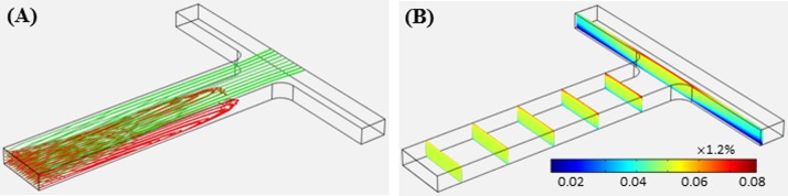
Isometric view of the numerically predicted 3D particle trajectories ((a), red and green lines are for diamagnetic and magnetic particles, respectively) and ferrofluid concentration contour ((b), over a series of cross-sectional slices) for simultaneous diamagnetic and magnetic particle trapping in ferrofluid flow through the T-shaped microchannel under a volume flow rate of 40 μl/h. Note that the bulk ferrofluid concentration far away from the T-junction is 0.05 × 1.2%.
A direct comparison of the experimental observations of particle trapping and ferrofluid nanoparticle buildup with the numerical simulations is presented in Fig. 7. The top-view composite image at the T-junction region (left panel, obtained by superimposing a sequence of snapshot images with a focal plane halfway the channel depth) is compared in Fig. 7(a) with the numerically predicted diamagnetic (red lines) and magnetic (green lines) particle trajectories that are both projected onto the horizontal plane (right panel). The experimentally observed V-shaped trapping pattern of diamagnetic particles is visually similar to the numerical prediction. Also, the experimental image of magnetic particle trapping (highlighted in Fig. 7(a), not clearly viewed due to their small size) appears to be qualitatively consistent with the predicted trajectories. The left panel in Fig. 7(b) shows a top-view snapshot image of the ferrofluid (in the absence of diamagnetic and magnetic particles) buildup at the T-junction region. This image was taken at the same focal plane as the particle image in Fig. 7(a) under an identical volume flow rate, which indicates that magnetic particles and ferrofluid are concentrated to the same location of the microchannel. Moreover, the experimentally observed ferrofluid nanoparticle buildup on the back wall of the T-junction is qualitatively simulated by the ferrofluid concentration contour in the right panel of Fig. 7(b).
C. Flow-tuned release of magnetically trapped diamagnetic and magnetic particles
The magnetically concentrated diamagnetic and magnetic particles in the T-shaped microchannel can be sequentially released from their respective trapping spots by tuning the ferrofluid flow rate. Fig. 8 shows the top-view snapshot (a) and composite (b) images of the flow-sweeping diamagnetic particles and the still-trapped magnetic particles when the volume flow rate is increased to 95 μl/h. Diamagnetic particles released in the main-branch are almost evenly split at the T-junction, which then travel through each side-branch in a stream nearby the front wall that is further away from the magnet. However, magnetic particles still remain trapped onto the back wall of the T-junction though at an enlarged region. These observations are simulated with a reasonable agreement by the particle trajectories at the same ferrofluid flow rate in Fig. 8(c). An isometric view of these predicted particle trajectories is displayed in Fig. 8(d). With a further increase in the ferrofluid flow rate, the trapping region of magnetic particles continues spreading and eventually reaches the two edges of the magnet. Following that part of the trapped magnetic particles start being flushed away by the strong shear flow. At a volume flow rate of 650 μl/h or more, magnetic particles can no longer be trapped at the T-junction which agrees well with the numerical prediction (data not shown). A quantitative comparison of the measured and predicted ferrofluid flow rates under the above-discussed three circumstances is presented in Table II. An overall good agreement is obtained except for the case of simultaneous diamagnetic and magnetic particle trapping due to the deficiency in the current numerical model (see the discussion in Section II B).
FIG. 8.

Selective release of the magnetically trapped diamagnetic particles in ferrofluid flow through a T-shaped microchannel at a volume flow rate of 95 μl/h: (a) and (b) the top-view snapshot and composite particle images; (c) the numerically predicted trajectories of diamagnetic (red) and magnetic (green) particles in the horizontal plane; (d) the isomeric view of the predicted 3D particle trajectories. The block arrows in (a) indicate the flow directions.
TABLE II.
Comparison of the experimentally measured and numerically predicted ferrofluid flow rates (μl/h) for diamagnetic and/or magnetic particle trapping.
| Trapping | Experiment | Simulation |
|---|---|---|
| Mag/diamag particles | 55 (±5) | 40 |
| Magnetic particles only | 95 (±5) | 100 |
| No particles | 650 (±50) | 700 |
V. CONCLUSIONS
We have demonstrated a new method for diamagnetic particle trapping in ferrofluid flows through a T-shaped microchannel via a single permanent magnet. Under a continuous supply of ferrofluid, the same device can also be used to trap magnetic particles simultaneously. Due to the induced negative and positive magnetophoresis, respectively, diamagnetic particles are trapped onto the bottom wall of the main-branch while magnetic particle are trapped into the top corner of the side-branch that is the nearest to the magnet center. These preconcentrated particles can then be sequentially released from the T-junction by simply increasing the ferrofluid flow rate. The proposed device may find potential applications in diamagnetic cell trapping1–4 and multi-sample bioassays.48–50 We have also developed a 3D numerical model to simulate the flow and concentration fields of the ferrofluid and track the motions of the two types of suspended particles under the influence of magnetic field. The predicted particle trajectories and ferrofluid nanoparticle buildup at the T-junction region agree reasonably with the experimentally obtained images under different ferrofluid flow rates. However, the observed circulation of the trapped diamagnetic particles is missing in the simulation. Moreover, the predicted maximum flow rate for simultaneous diamagnetic and magnetic particle trapping is significantly smaller than the experimentally measured value. These discrepancies have been attributed to the neglect of particle and ferrofluid effects on magnetic and flow fields in the 3D numerical model. The consideration of these effects will couple the ferrofluid concentration field with the ferrofluid flow field and magnetic field. A full numerical model is currently under development.
ACKNOWLEDGMENTS
This work was supported in part by NSF under Grant No. CBET-1150670 (X. Xuan). The support from University 111 Project of China under Grant No. B08046 is also gratefully acknowledged (Y. Song).
References
- 1. Ramadan Q. and Gijs M. A., Microfluid. Nanofluid. 13, 529–542 (2012). 10.1007/s10404-012-1041-4 [DOI] [Google Scholar]
- 2. Johann R. M., Anal. Bioanal. Chem. 385, 408–412 (2006). 10.1007/s00216-006-0369-6 [DOI] [PubMed] [Google Scholar]
- 3. Nilsson J., Evander M., Hammarstrom B., and Laurell T., Anal. Chim. Acta 649, 141–157 (2009). 10.1016/j.aca.2009.07.017 [DOI] [PubMed] [Google Scholar]
- 4. Pratt E. D., Huang C., Hawkins B. G., Gleghorn J. P., and Kirby B. J., Chem. Eng. Sci. 66, 1508–1522 (2011). 10.1016/j.ces.2010.09.012 [DOI] [PMC free article] [PubMed] [Google Scholar]
- 5. Juncker D., Schmid H., and Delamarche E., Nat. Mater. 4, 622–628 (2005). 10.1038/nmat1435 [DOI] [PubMed] [Google Scholar]
- 6. Hamblin M. N., Xuan J., Maynes D., Tolley H. D., Belnap D. M., Woolley A. T., Lee M., and Hawkins A. R., Lab Chip 10, 173–178 (2010). 10.1039/B916746C [DOI] [PubMed] [Google Scholar]
- 7. Watarai H., Annu. Rev. Anal. Chem. 6, 353–378 (2013). 10.1146/annurev-anchem-062012-092551 [DOI] [PubMed] [Google Scholar]
- 8. Nordin M. and Laurell T., Lab Chip 12, 4610–4616 (2012). 10.1039/c2lc40629b [DOI] [PubMed] [Google Scholar]
- 9. Chen Y., Li S., Gu Y., Li P., Ding X., McCoy J. P., Levine S. J., Wang L., and Huang T. J., Lab Chip 14, 924–930 (2014). 10.1039/c3lc51001h [DOI] [PMC free article] [PubMed] [Google Scholar]
- 10. Pethig R., Biomicrofluidics 4, 022811 (2010). 10.1063/1.3456626 [DOI] [PMC free article] [PubMed] [Google Scholar]
- 11. Church C., Zhu J., Huang G., Tzeng T. R., and Xuan X., Biomicrofluidics 4, 044101 (2010). 10.1063/1.3496358 [DOI] [PMC free article] [PubMed] [Google Scholar]
- 12. Salmanzadeh A., Sano M. B., Gallo-Villanueva R. C., Roberts P. C., Schmelz E. M., and Davalos R. V., Biomicrofluidics 7, 011809 (2013). 10.1063/1.4788921 [DOI] [PMC free article] [PubMed] [Google Scholar]
- 13. Harrison H., Lu X., Patel S., Thomas C., Todd A., Johnson M., Raval Y., Tzeng T. R., Song Y., Wang J., Li D., and Xuan X., Analyst 140, 2869–2875 (2015). 10.1039/C5AN00105F [DOI] [PubMed] [Google Scholar]
- 14. Williams S. J., Kumar A., and Wereley S. T., Lab Chip 8, 1879–1882 (2008). 10.1039/b810787d [DOI] [PubMed] [Google Scholar]
- 15. Kayani A., Khoshmanesh K., Ward S. A., Mitchell A., and Kalantar-zadeh K., Biomicrofluidics 6, 031501 (2012). 10.1063/1.4736796 [DOI] [PMC free article] [PubMed] [Google Scholar]
- 16. Zhao C., Xie Y., Mao Z., Zhao Y., Rufo J., Yang S., Guo F., Mai J. D., and Huang T. J., Lab Chip 14, 384–391 (2014). 10.1039/C3LC50748C [DOI] [PMC free article] [PubMed] [Google Scholar]
- 17. Pamme N., Lab Chip 6, 24–38 (2006). 10.1039/B513005K [DOI] [PubMed] [Google Scholar]
- 18. Suwa M. and Watarai H., Anal. Chim. Acta 690, 137–147 (2011). 10.1016/j.aca.2011.02.019 [DOI] [PubMed] [Google Scholar]
- 19. Nguyen N. T., Microfluid. Nanofluid. 12, 1–16 (2012). 10.1007/s10404-011-0903-5 [DOI] [Google Scholar]
- 20. Watarai H., Suwa M., and Iiguni Y., Anal. Bioanal. Chem. 378, 1693–1699 (2004). 10.1007/s00216-003-2354-7 [DOI] [PubMed] [Google Scholar]
- 21. Cao Q., Han X., and Li L., Lab Chip 14, 2762–2777 (2014). 10.1039/c4lc00367e [DOI] [PubMed] [Google Scholar]
- 22. Hejazian M., Li W., and Nguyen N. T., Lab Chip 15, 959–970 (2015). 10.1039/C4LC01422G [DOI] [PubMed] [Google Scholar]
- 23. Plouffe B. D., Lewis L. H., and Murthy S. K., Biomicrofluidics 5, 013413 (2011). 10.1063/1.3553239 [DOI] [PMC free article] [PubMed] [Google Scholar]
- 24. Yassine O., Gooneratne C. P., Abu Smara D., Li F., Mohammed H., Merzaban J., and Kosel J., Biomicrofluidics 8, 034114 (2014). 10.1063/1.4883855 [DOI] [PMC free article] [PubMed] [Google Scholar]
- 25. Liu C., Stakenborg T., Peeters S., and Lagae L., J. Appl. Phys. 105, 102014 (2009) 10.1063/1.3116091. [DOI] [Google Scholar]
- 26. Chung J., Issadore D., Ullal A., Lee K., Weissleder R., and Lee H., Biomicrofluidics 7, 054107 (2013). 10.1063/1.4821923 [DOI] [PMC free article] [PubMed] [Google Scholar]
- 27. Osman O., Toru S., Dumas-Bouchiat F., Dempsey N. M., Haddour N., Zanini L.-F., Buret F., Reyne G., and Frénéa-Robin M., Biomicrofluidics 7, 054115 (2013). 10.1063/1.4825395 [DOI] [PMC free article] [PubMed] [Google Scholar]
- 28. Zhu T., Cheng R., and Mao L., Microfluid. Nanofluid. 11, 695–701 (2011). 10.1007/s10404-011-0835-0 [DOI] [Google Scholar]
- 29. Liang L. and Xuan X., Microfluid. Nanofluid. 13, 637–643 (2012). 10.1007/s10404-012-1003-x [DOI] [Google Scholar]
- 30. Zeng J., Chen C., Vedantam P., Brown V., Tzeng T., and Xuan X., J. Micromech. Microeng. 22, 105018 (2012). 10.1088/0960-1317/22/10/105018 [DOI] [Google Scholar]
- 31. Liang L. and Xuan X., Biomicrofluidics 6, 044106 (2012). 10.1063/1.4765335 [DOI] [PMC free article] [PubMed] [Google Scholar]
- 32. Zhu T., Cheng R., Lee S. A., Rajaraman E., Eiteman M. A., Querec T. D., Unger E. R., and Mao L., Microfluid. Nanofluid. 13, 645–654 (2012). 10.1007/s10404-012-1004-9 [DOI] [PMC free article] [PubMed] [Google Scholar]
- 33. Zeng J., Deng Y., Vedantam P., Tzeng T., and Xuan X., J. Magn. Magn. Mater. 346, 118–123 (2013). 10.1016/j.jmmm.2013.07.021 [DOI] [Google Scholar]
- 34. Tarn M. D., Hirota N., Iles A., and Pamme N., Sci. Technol. Adv. Mater. 10, 014611 (2009). 10.1088/1468-6996/10/1/014611 [DOI] [PMC free article] [PubMed] [Google Scholar]
- 35. Rodriguez-Villarreal A. I., Tarn M. D., Madden L. A., Lutz J. B., Greenman J., Samitier J., and Pamme N., Lab Chip 11, 1240–1248 (2011). 10.1039/C0LC00464B [DOI] [PubMed] [Google Scholar]
- 36. Liang L., Zhu J., and Xuan X., Biomicrofluidics 5, 034110 (2011). 10.1063/1.3618737 [DOI] [PMC free article] [PubMed] [Google Scholar]
- 37. Zhu T., Lichlyter D. J., Haidekker M. A., and Mao L., Microfluid. Nanofluid. 10, 1233–1245 (2011). 10.1007/s10404-010-0754-5 [DOI] [Google Scholar]
- 38. Zhu J., Liang L., and Xuan X., Microfluid. Nanofluid. 12, 65–73 (2012). 10.1007/s10404-011-0849-7 [DOI] [Google Scholar]
- 39. Liang L., Zhang C., and Xuan X., Appl. Phys. Lett. 102, 234101 (2013). 10.1063/1.4810874 [DOI] [Google Scholar]
- 40. Cheng R., Zhu T., and Mao L., Microfluid. Nanofluid. 16, 1143–1154 (2014). 10.1007/s10404-013-1280-z [DOI] [Google Scholar]
- 41. Zhu G. P., Hejiazan M., Huang X. Y., and Nguyen N. T., Lab Chip 14, 4609–4615 (2014). 10.1039/C4LC00885E [DOI] [PubMed] [Google Scholar]
- 42. Zhu T., Cheng R., Liu Y., He J., and Mao L., Microfluid. Nanofluid. 17, 973–982 (2014). 10.1007/s10404-014-1396-9 [DOI] [Google Scholar]
- 43. Winkleman A., Gudiksen K. L., Ryan D., and Whitesides G. M., Appl. Phys. Lett. 85, 2411–2413 (2004). 10.1063/1.1794372 [DOI] [Google Scholar]
- 44. Feinstein E. and Prentiss M., J. Appl. Phys. 99, 064901 (2006). 10.1063/1.2179196 [DOI] [Google Scholar]
- 45. Peyman S. A., Kwan E. Y., Margarson O., Iles A., and Pamme N., J. Chromatogr. A 1216, 9055–9062 (2009). 10.1016/j.chroma.2009.06.039 [DOI] [PubMed] [Google Scholar]
- 46. Zeng J., Chen C., Vedantam P., Tzeng T. R., and Xuan X., Microfluid. Nanofluid. 15, 49–55 (2013). 10.1007/s10404-012-1126-0 [DOI] [Google Scholar]
- 47. Wilbanks J. J., Kiessling G., Zeng J., Zhang C., and Xuan X., J. Appl. Phys. 115, 044907 (2014). 10.1063/1.4862965 [DOI] [Google Scholar]
- 48. Smistrup K., Tang P. T., Hansen O., and Hansen M. F., J. Magn. Magn. Mater. 300, 418–426 (2006). 10.1016/j.jmmm.2005.05.031 [DOI] [Google Scholar]
- 49. Bronzeau S. and Pamme N., Anal. Chim. Acta 609, 105–112 (2008). 10.1016/j.aca.2007.11.035 [DOI] [PubMed] [Google Scholar]
- 50. Tarn M. D., Peyman S. A., and Pamme N., RSC Adv. 3, 7209–7214 (2013). 10.1039/c3ra40237a [DOI] [Google Scholar]
- 51. Puri I. K. and Ganguly R., Annu. Rev. Fluid Mech. 46, 407–440 (2014). 10.1146/annurev-fluid-010313-141413 [DOI] [Google Scholar]
- 52.EMG 408 ferrofluid from www.Ferrotec.com.
- 53. Rosensweig R. E., Annu. Rev. Fluid Mech. 19, 437–463 (1987). 10.1146/annurev.fl.19.010187.002253 [DOI] [Google Scholar]
- 54. Furlani E. P., Permanent Magnet and Electromechanical Devices: Materials, Analysis, and Applications ( Academic Press, New York, 2001). [Google Scholar]
- 55. Han X., Feng Y., Cao Q., and Li L., Microfluid. Nanofluid. 18, 1209–1220 (2015). 10.1007/s10404-014-1516-6 [DOI] [Google Scholar]
- 56. Zhu G. and Nguyen N. T., Lab Chip 12, 4772–4780 (2012). 10.1039/c2lc40818j [DOI] [PubMed] [Google Scholar]