Reconstructing tumor-wise protein expression in tissue microarray studies using a Bayesian cell mixture model

Abstract

Motivation: Tissue microarrays (TMAs) quantify tissue-specific protein expression of cancer biomarkers via high-density immuno-histochemical staining assays. Standard analysis approach estimates a sample mean expression in the tumor, ignoring the complex tissue-specific staining patterns observed on tissue arrays.

Methods: In this article, a cell mixture model (CMM) is proposed to reconstruct tumor expression patterns in TMA experiments. The concept is to assemble the whole-tumor expression pattern by aggregating over the subpopulation of tissue specimens sampled by needle biopsies. The expression pattern in each individual tissue element is assumed to be a zero-augmented Gamma distribution to assimilate the non-staining areas and the staining areas. A hierarchical Bayes model is imposed to borrow strength across tissue specimens and across tumors. A joint model is presented to link the CMM expression model with a survival model for censored failure time observations. The implementation involves imputation steps within each Markov chain Monte Carlo iteration and Monte Carlo integration technique.

Results: The model-based approach provides estimates for various tumor expression characteristics including the percentage of staining, mean intensity of staining and a composite meanstaining to associate with patient survival outcome.

Availability: R package to fit CMM model is available at http://www.mskcc.org/mskcc/html/85130.cfm

Contact: shenr@mskcc.org

Supplementary information: Supplementary data are available at Bioinformatics online.

1 INTRODUCTION

A tissue microarray (TMA) experiment measures tumor-specific protein expression via high-density immunohistochemical (IHC) staining assays, allowing simultaneous evaluation of hundreds of patient samples on a single array (Kononen et al., 1998). Since their initial development, TMA-based expression studies have quickly become an integral part of cancer biomarker development (Divito et al., 2004; Rubin et al., 2005; Seligson et al., 2005). A typical tissue array comprises up to 1000 tiny biopsy tissue elements (tissue cores) with multiple elements corresponding to repeated sampling from individual tumors. Expression data consisting the IHC staining intensity and staining percentage are obtained on individual cores. Such core-level measures can display substantial within-tumor variability. Liu et al. (2004) considered various pooling methods, such as the mean, median, minimum and maximum of the core-level data. They found different choices of pooling method led to disparate results in Cox regression analysis. Demichelis et al. (2006) incorporated such within-tumor heterogeneity in a hierarchical Bayes model for tumor classification and showed improved performance over the naive classifier. For survival outcome, Shen et al. (2008) proposed a measurement error approach to jointly model the repeated expression measures and patient's survival. The joint model was shown to outperform the naive method and a two-stage approach in estimating the hazard ratio in Cox regression models.

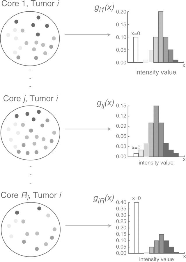
In this study, we propose a novel idea of modeling the expression data. We introduce the concept of a cell mixture model (CMM). As will be discussed later, the error model in the previous paper (Shen et al., 2008) is a special case of the new framework. As illustrated in Figure 1, the basic idea of the CMM model can be decomposed into the following aspects: (1) a tumor is represented by a population of R_i needle biopsy samples (the total sampling capacity of a tumor; 2) the expression values in each individual tissue core is a mixture distribution with a point mass at zero (the non-staining area; 3) the whole-tumor expression can be recapitulated by adding up (e.g. weighted summation of) the distributions of the expression values in all the needle biopsy samples (or commonly referred to as tissue cores in TMA study). The mathematical description will be put forward in the Section 2.

Fig. 1.

A conceptual model for the whole tumor. Each tumor i represented by a population of R_i tissue cores.

There are difficulties of implementing such a mixture model in TMA expression data. First, the experimental data are only collected on a small number (r_i out of R_i) of random sample of tissue cores in tumor i. Generally speaking, the number of measured cores r_i often averages from 3–5 whereas R_i can be in the hundreds, though both may vary proportionate to the size of the tumor. Second, each core is a very small subarea measured in millimeters compared to the whole tumor which averages around 1–2 cm (prostate tumors). When our interest is to obtain accurate estimates for tumor- and core-level expression characteristics, sample-based methods will not be satisfactory. An analogy is in estimation of the characteristics of the population in the United States with data collected in three representative cities. In survey sampling problems, small area estimation often involves parameter estimation for a small sub-population of interest. Hierarchical Bayes (HB) and empirical Bayes (EB) approaches have been effective with continuous data. For a thorough review of various methods, see Ghosh and Rao (1994), Rao (1999) and Pfreffermann (2002). For a unified analysis of discrete and continuous data, Ghosh et al. (1998) present hierarchical Bayes generalized linear models. The idea of Bayesian predictive inference and Markov chain Monte Carlo integration is particularly useful for our problem at hand. In this study, we extend the implementation to a zero-point mass mixture distribution under the CMM model. Details of constructing the CMM expression estimators will be discussed in Section 2.

Associating tumor-wise expression features with patient survival information is of scientific interest in TMA studies. Therefore accurate estimation of the disease risk associated with a biomarker is essential. To achieve this, a joint modeling approach would be most effective in which the expression data and the survival data are simultaneously modeled. Markov chain Monte Carlo methods offer a convenient framework for complex problems where analytic solutions are often unavailable or cumbersome. As will be discussed in detail in Section 2, linking the CMM model on the expression data with survival requires an imputation step within each Markov Chain Monte Carlo (MCMC) iteration where draws are obtained from posterior predictive distributions.

2 METHODS

2.1 Notation and the model

Figure 1 describes the concept of the CMM. The cartoon illustrates a tumor being dissected into a population of R_i tissue core samples. Each core j (j=1,…,R_i) captures a sample of cells stained at different intensities. Let a_ij(x)denote the number of cells measured at staining intensity x,x∈[0,M] in core j of tumor i. Thus the density function of x can be expressed as g_ij(x)=a_ij(x)/n_ij, where n_ij is the total number of cells in core j of tumor i. The total number of cells measured is N_i=∑_l=1^R_i n_ij. In Figure 1, each histogram is informative of g_ij, which is assumed to be a mixture density with a point mass at zero for the non-staining area and some density function f(·) for the positively stained area. In particular,

(2.1)

where π_ijdenotes the proportion of staining; μ_ij,σ_ij are mean and variance parameters associated with the density f. Subsequently, the tumor-wise density function g_i(x) is aggregated over all the g_ij(x)′s:

(2.2)

where ω_ij=n_ij/N_i and ∑_l=1^R_i ω_ij=.

2.2 Description of the data

The tumor sampling scheme in TMA experiments has a ‘geographical’ clustered sampling structure. Consider each tumor as a population of cells. Small areas of 0.6 mm (cores) are taken from the tumor where cells within each area are measured for protein expression. Let X_ijk be the resulting intensity measure in tumor (i=1,…,m), core j (j=1,…,r_i), and cell k (k=1,…,n_ij). It needs to be pointed out that X_ijk is an idealized measure where measurements can be taken per cell. The current technology instead provides a crude mean intensity measure for cells that have non-zero intensity

per core. As illustrated in Figure 2, Y_ij is the actual observed data whereas the cell-level data are latent. The empirical estimate of μ_ij is y_ij. For the zero-mass part, we observe the number of positively staining cells and the number of non-staining cells which are

respectively. And n_ij=n_1ij+n_0ij will be the total number of cells measured in tumor i core j. The empirical estimate of π_ij is n_1ij/n_ij.

Fig. 2.

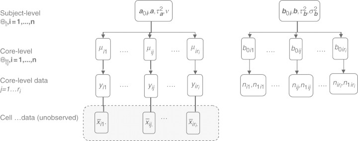
The CMM structure.

2.3 A hierarchical zero-augmented Gamma model

In this section, we introduce a zero-augmented Gamma (hZAG) model for the observed data.

2.3.1 Modeling the positive staining intensity

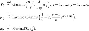
We start by assuming X_ijk∣X_ijk>0 follow a Gamma distribution G(1/δ,δμ_ij) with mean μ_ij, variance δμ_ij² and the coefficient of variation For identifiability issue, we set δ=0.2 which is a reasonable choice based on the real datasets. The choice of Gamma distribution leads to a standardized Gamma distribution for Y_ij. In simulation, we did not find serious model misspecification problems for the Gamma model when simulating Y_ij from a log-normal distribution (Supplementary Fig. 1). A Gamma-Inverse Gamma-Normal hierarchical model is set up as follows:

(2.3)

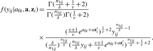
In this model, {μ_i1,…,μ_iri} denotes the vector of core-level random effects for subject i and {a₀₁,…,a_0n} denotes the vector of subject-level random effects. Given the Gamma-Inverse Gamma conjugacy, the marginal densities integrated over μ_ij has the following analytic form:

(2.4)

where z_i is tumor-level covariates and a is the associated coefficients.

2.3.2 Modeling the point mass at zero

To model the point mass at zero in the mixture density of Equation (2.1), we assume the following hierarchical structure:

(2.5)

where b_0i∼N(0,τ²_b), ɛ_ij∼N(0,σ²_b) and z_i can be the same or different than those included in Equation (2.3). Let b_0ij=logit(π_ij) such that π_ij=exp(b_0ij)/(1+exp(b_0ij)).

The core- and subject-level parameter space are

respectively (as illustrated in Fig. 2). The likelihood function treating the latent quantities as parameters can be written as:

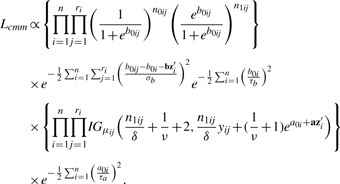(2.6)

To complete the hierarchy for the Bayesian model, the following prior distributions are specified as:

(2.7)

where N(·) denotes Normal distribution and G(·) denotes Gamma distribution. Posterior inference will then be based on the joint posterior distribution f(Θ_ij, Θ_i∣D). Gibbs sampling is used to iteratively sample from the full conditionals of each parameter given the rest of the parameters and the data.

2.4 Estimation of tumor-wise expression characteristics

In this section, we focus on estimating the tumor-wise protein expression characteristics. Three quantities are of interest: the tumor-wise proportion of staining (π_i), mean intensity of staining (μ⁺_i) and a composite intensity (μ_i). Under the proposed CMM assumptions, these quantities are defined as

(2.8)

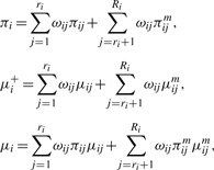
respectively. Here π_ij=exp(b_0ij)/(1+exp(b_0ij)). For the rest of the article, we use h(Θ_ij), where Θ_ij=(b_0ij,μ_ij), as a general notation for the above expression characteristics. Assume independence among the cores and, without loss of generality, assume the first r_i cores from the i-th tumor are observed and the rest of the cores are not observed, we decompose h(Θ_ij) as

(2.9)

where the first components of the expansion are estimable given the data D=(y_ij, n_1ij, n_ij: i=1,…,n; j=1,…,r_i), and the second components involve latent quantities Θ_ij^m where data are not observed for core j (j=r_i+1,…,R_i).

2.4.1 The CMM model-based estimator

To obtain a CMM model-based estimate of h(Θ_ij), we propose a Bayesian framework. (1) The first com-ponent of Equation (2.9) is computed based on a set of draws Θ^(g)_ij={b^(g)_0ij, μ^(g)_ij: g=1,…,G} from the posterior density f(Θ_ij∣Θ_i,D) for j=1,…,r_i. The posterior means ; , and are then readily obtained from the posterior samples. (2) Let Θ_ij^m=(b_0ij^m, μ_ij^m)—the parameter vector involved in the second component of Equation (2.9). In the absence of knowledge about Θ_ij^m, we replace the latent quantities with their expectation E[Θ_ij^m∣D]. To calculate this, we use the posterior predictive density function

Using Monte Carlo integration technique, we first draw Θi from their joint posterior distribution f(Θi∣D) and then simulate Θ_ij^m according to Equations (2.3) and (2.5). Let {Θ^(p)_ij: p=1,…,P} be the set of predictive draws. The followingquantities can then be computed:

(2.10)

Similarly, we simulate a set of {μ_ij^(p), m=1,…,P}, given using Equation (2.3) and obtain

(2.11)

Finally, the composite mean at the g-th iteration is computed as

(2.12)

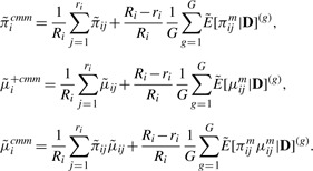
These are essentially imputation steps within each MCMC iteration. Assuming equal weights ω_ij≡1/R_i, the CMM estimates are

(2.13)

Since R_i≫r_i, we let (R_i−r_i)/R_i→1 and 1/R_i→0 such that the second term is used as the estimate. This circumvents the need to specify the value of R_i which is a theoretical construct to motivate the model and not observed.

2.4.2 Sample-based estimates

The sample-based estimates are derived as:

(2.14)

These sample-based estimates are implied by the proposed model by setting σ²_b=0 in Equation (2.5) and ν=0 in Equation (2.3) such that homogeneity is assumed across cores within a tumor. These estimates are unbiased when the sample cores have the same characteristics as the tumor.

2.5 Joint analysis with patient survival outcome

In TMA studies, the ultimate interest is to associate the tumor expression characteristics to patient survival data in the following proportional hazards model form:

(2.15)

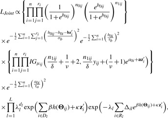
adjusting for clinical covariates zi. A joint modeling approach would be the most effective way to obtain accurate estimates of disease risks associated with a biomarker. To extend the CMM model into a joint model with censored failure time data, we use a piecewise constant hazards model in which the time axis is partitioned into L disjoint intervals, I₁,…,I_L, where I_l=[a_l−1,a_l) with a₀<t_i and a_L>t_i for all i=1,…,n. L is chosen such that each interval contains approximately equal number of events. Assume a constant baseline hazard in the l-th interval, let λ₀(t)=λ_l for t∈I_l. R_l is the set at risk at the beginning of interval l; d_l is the number of failures in interval l and Δ_il=min(t_i, a_l)–a_l−1. By treating the latent variables b_0ij, μ_ij as a set of parameters in a Bayesian framework, the joint likelihood function is given by

(2.16)

where Θ_ij=(b_0ij, μ_ij). The following priors in addition to those specified in (2.7) arechosen:

(2.17)

The parameter spaces are expanded to:

(2.18)

The full conditional of β is given by

(2.19)

where at the g-th MCMC iteration, computation of h(Θ_ij) involves predictive draws and Monte Carlo integration as discussed in the previous section. The details of the MCMC implementation can be found in (Shen, 2007).

3 SIMULATION STUDY

3.1 Simulation setup

In the simulation study, we assign parameter values in the simulation to mimic those for the real datasets. In particular, the parameter values under the hZAG model are specified as follows: τ²_a=0.01, σ²_b=1,τ²_b=1. The model has one covariate Z_1i simulated from N(0,1) with associated model coefficient a₁=0.5, b₁=0.5. For each tumor, r_i is simulated from Binomial(10, 0.5). Simulation of R_i, the total sampling capacity of a tumor, is relatively subjective as no information is available. We simulate R_i from a Binomial(200, p_i) where p_i is allowed to vary with covariates such as tumor size. The survival time T_i is simulated from a proportional hazards model in the following form

(3.1)

with λ₀(t)≡1. The censoring time is simulated from an independent exponential distribution that results in a 30% censoring proportion. Proper priors were used in the CMM model by setting a_k, b_k∼N(0,1000) and τ⁻²_a, τ⁻²_b, σ⁻²_b,ν∼Gamma(0.001,0.001). Similarly in the survival model, prior specifications are β, {κ_j}₁^J∼N(0,1000) and {λ_l}₁^L∼Gamma(0.001,0.001). All programming is done using the R programming language. Convergence is fast for μ⁺_i due to a closed form solution and therefore the elimination of the Monte Carlo imputation step within each MCMC iteration. We discarded the first 4000 iterations as the burn-in period. For π_i and μ_i, we used a 10 000 burn-in period. Convergence is monitored using traceplots. Every 10th sample is then retained to achieve a total of 1000 samples, from which posterior mean and SD were calculated. Each simulation consisted of 100 replicate data, each of n=100 subjects. Results are summarized over replicated datasets.

3.2 Simulation results

The interest in this section is to estimate the Cox regression coefficient β in Equation (3.1). The hazard ratio is exp(β). Three approaches are compared: a naive method where the sample-based expression estimates are plugged in a Cox model; a two-stage CMM method where the CMM estimates are plugged in the Cox model and the joint modeling approach based on the joint likelihood (2.16). The first two methods are considered two-stage methods as compared with the joint model. The two-stage methods have several major limitations. First, the survival information is not used in the CMM model to reconstruct tumor expression, which can cause bias and efficiency loss in estimating β in the second stage. Second, the uncertainty of estimating the expression quantity is not assimilated in the second stage, leading to overoptimistic standard error estimates of . The joint modeling approach concurrently updates the CMM model and the survival model by iteratively sampling through the joint posterior distribution of the combined parameter space. We therefore expect more accurate inference from the joint model. In Table 1, the top panel simulates β_πi=2, β_μ⁺i=0, β_μi=0, the middle panel assumes β_πi=0, β_μ⁺i=2.5, β_μi=0 and the bottom panel assumes β_πi=0, β_μ⁺i=0, β_μi=1.8. It is evident that the joint model performs best in terms of the estimates and coverage probabilities for .

Table 1.

Cox regression

h(Θij)	true β				coverage
πi	2	2.06	0.24	0.23	0.97
		1.48	0.23	0.18	0.27
		1.60	0.22	0.22	0.53
Joint model		2.06	0.32	0.40	0.97
μ+i	2.5	2.50	0.30	0.26	0.93
		1.43	0.25	0.23	0.39
		2.07	0.27	0.23	0.44
Joint model		2.48	0.55	0.49	0.94
μi	1.8	1.82	0.21	0.20	0.95
		1.40	0.18	0.16	0.48
		1.68	0.16	0.19	0.79
Joint model		1.75	0.41	0.47	0.95

Results are summarized over 100 simulated datasets each of n=100.

4 CASE STUDY USING PROSTATE CANCER TMA EXPERIMENTS

4.1 Data description and model fit

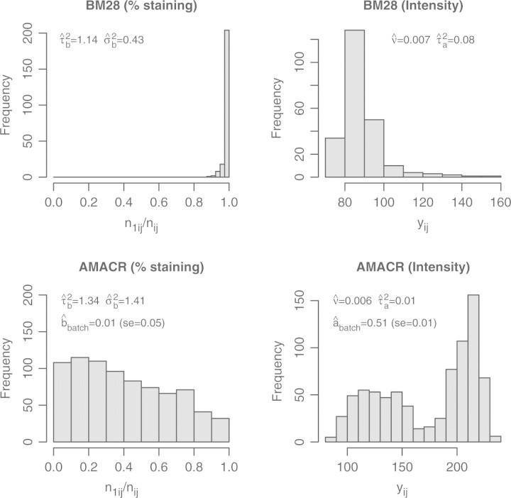
We apply the CMM model to two prostate cancer TMA datasets used in Shen et al. (2008). The protein expression of two cancer biomarkers, AMACR and BM28, were measured using tissue arrays constructed on 203 prostate tumors from a surgical cohort who underwent radical prostatectomy at the University of Michigan as a primary therapy for clinically localized prostate cancer diagnosed between 1994 and 1998. The outcome of interest is prostate-specific antigen (PSA) failure. Gleason score and pathologic stage are included as the clinical covariates Z_i. A batch effect is added to the AMACR dataset, as evident in Figure 3, the staining intensity distribution is bimodal. In Rubin et al. (2005), an array-wise normalization was performed to eliminate the batch effect resulting from experiment-to-experiment variation of immunohistochemical staining. For MCMC convergence of the joint model, we use the first 10 000 draws as burn-in, and retain every 20th draw till 1000 samples are collected for inference. To evaluate the model fit, we plotted fitted density function in four tumors each has relatively ‘abundant’ number of cores to illustrate the ‘reconstructed’ expression profile based on the CMM model. Supplementary Figure 2 did not suggest extremely unreasonable fit.

Fig. 3.

Histograms of the percentage of staining and the intensity of staining. The estimated variance parameters in the CMM model are indicated in the plots. For the AMACR data, the batch effect for the Gamma-Inverse-Gamma model is listed.

4.2 BM28 expression characteristics and patient survival

Figure 3 suggests that BM28 is a homogeneously stained marker. All of the52 tumors showed over 94% staining, suggesting the percentage of staining is not an informative measure for BM28. We therefore focus on analyzing the intensity of the staining of this gene biomarker. This is clarified in Section 4.2.

The top panel of Table 2 describes the performance of Cox regression models relating the estimated mean intensity of BM28 to PSA recurrence adjusting for Gleason score and pathological stage of the tumor. Among the two stage estimation procedures of β, the CMM estimator of μ⁺_i does not perform better than the sample-based estimator. It is likely that the CMM estimates in the dataset does not approximate the true expression quantity significantly better than would the sample-based estimates when the within-subject variation ν is small (). The joint model estimate is however more than two times larger than those under the two-stage estimation. The estimated hazard ratio under the joint model is 4.4 (95% CI:1.6–11.7) compared with 1.9 (95% CI: 1.2–3.0) estimated under two-stage methods. However, a hypothesis test of H₀:β=0 would give similar conclusions as the estimated standard error from the joint model is also substantially larger than those from the two-stage estimation. After controlling for Gleason and pathological stage of the disease, the mean intensity of BM28 staining in the tumor is a significant predictor of prostate cancer PSA recurrence. A further notion is that these results are consistent with those observed under a measurement error model in Shen et al. (2008). The underlying Gamma-Inverse-Gamma assumption on the intensity measure versus the log-normal assumption adopted there does not seem to have large influence on estimating the Cox regression coefficient β in the joint model.

Table 2.

Case study using prostate cancer TMA datasets

	Sample-based		CMM (2stg)		Joint model
BM28 (n=52)
μ+i	0.668	0.232	0.630	0.236	1.481	0.501
Gleason	0.666	0.601	0.683	0.561	0.592	0.558
Stage	0.938	0.507	0.837	0.535	0.822	0.501
AMACR (n=203)
πi	0.827	0.358	1.284	0.539	1.778	0.586
μ+i	−1.132	0.464	−0.554	0.402	−0.488	0.389
μi	−0.736	0.457	−1.008	0.458	−2.372	0.728
Gleason	1.237	0.418	1.177	0.42	1.025	0.513
Stage	1.345	0.298	1.254	0.298	1.276	0.293

Prediction of patient PSA recurrence using tumor-wise protein expression estimates.

4.3 AMACR expression characteristics and patient survival

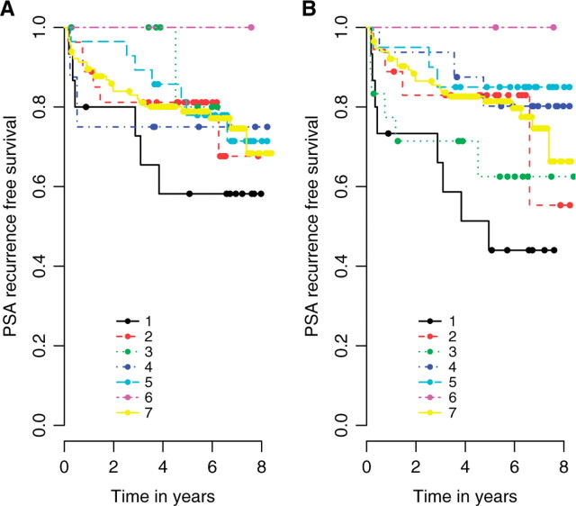
Table 2 summarizes the results in the AMACR dataset. A distinct feature is the interactions among the expression characteristics. The predictive value of π_i depends on the values of μ⁺_i and μ_i, and vice versa. In a simulation study when similar coefficient values are assigned to the three expression features according to the real data, we found that noise-inflated expression estimates (e.g. sample-based) would in the same fashion attenuate β_πi and β_μi, and yet overestimate β_μ⁺i. Figure 4 reveals the complexity of AMACR protein expression as a predictor of PSA recurrence outcome. Each of the three expression estimates are dichotomized into two risk groups using the lower quartile as cutoff, resulting in a total of eight combinations (though one group has 0 observations). Overall, B demonstrates better differentiation of risk groups compared to A. In both figures, tumors demonstrating low staining proportion, low intensity and low composite intensity (curve 1) has the highest recurrence risk of all. One significant difference between A and B lies in curves 3 and 4. The joint model has generated substantially different estimates of the recurrence risks for these two groups compared with sample-based methods.

Fig. 4.

Kaplan–Meier plots. Patients are categorized into risk groups based on the AMACR expression estimates [(A) sample-based, (B) joint model]. The lower quartiles are used for dichotomization. 1. low π_i, low μ⁺_i, low μ_i; 2. low π_i, high μ⁺_i, low μ_i; 3. low π_i, high μ⁺_i, high μ_i; 4. high π_i, low μ⁺_i, low μ_i; 5. high π_i, low μ⁺_i, high μ_i; 6. high π_i, high μ⁺_i, low μ_i; 7. high π_i, high μ⁺_i, high μ_i.

5 DISCUSSION

A CMM is proposed to reconstruct tumor expression characteristics from TMA data. The concept is to assemble the whole-tumor expression pattern from the subpopulation of tissue cores. We let each individual core density adopt a zero-augmented Gamma density function to describe the proportion of non-staining and the intensity of the positive staining, respectively. A two-stage approach and a joint model are presented to link the CMM expression model patient survival outcome. The implementation of the joint model involves imputation steps within each MCMC iteration and Monte Carlo integration technique. Simulation studies show that the joint model can effectively reduce the attenuation of the disease risk estimates evident in two-stage methods. In addition, when interactions among the expression features exist, relating noise-inflated expression estimates to survival can lead to misleading results. Applying the joint model effectively avoids an erroneous interpretation of the risk estimates. So in conclusion, inference based on the joint likelihood is preferred over the two-stage approach.

Using notations from the current article, the error model proposed in Shen et al. (2008) concerns a ‘true’ protein expression level y^*_i in tumor i. The core-level data vector of staining intensity measures D=(y_i1,…,y_iri) are modeled as repeated measures (error-prone) of the truth y^*_i. The objective is then to assess the prognostic value of this ‘true’ expression quantity y^*_i given D in survival regression models. The measurement error model has the benefit of model simplicity by simplifying the data structure using an inferred ‘true’ expression quantity. In addition, the proportion of non-staining captured by the data vector (n_1ij,n_ij:j=1,…,r_i) was not explicitly modeled in that study.

The CMM model in the current study is fundamentally different in concept than the error model. Here, we consider a full distribution of the biomarker expression in tumor i with density function g_i(x), composed of a mixture pattern of non-staining (x=0) and positive staining (x>0). This densities characteristics, such as (though not limited to) E[x∣x=0], E[x|x>0] and E[x] are then explored as predictors of that patient's survival outcome. Those three characteristics correspond to 1−π_i, μ⁺_i and μ_i, respectively in Equation (2.9).

To make a connection, the quantity y^*_i in the error model bears similarity to the positive mean μ⁺_i under the CMM framework when we let the dispersion δ of the Gamma distribution in Equation (2.3) go to zero. So to some degree, the error model can be considered a special case of the CMM model.

Another novel aspect of the CMM model is the idea of constructing the tumor-wise density function g_i(x) as a weighted summation of the core density functions in the form of Equation (2.2). Although we used equal weights in this study, it is straightforward to implement differential weights if certain cores are regarded by pathologist's review as more important or representative than others. In other scenarios, it is also plausible that one would wish to down-weight cores, for example, because of stroma contamination.

Naturally the CMM model is a more challenging implementation. Some of the major difficulties of fitting CMM model are (1) the requirement of cumbersome imputation steps by Monte Carlo integration within each MCMC iteration and (2) more parameters in the model thatneed careful monitoring for convergence.

REFERENCES

- Demichelis F, et al. A hierarchical naive Bayes model for handling sample heterogeneity in classification problems: an application to tissue microarrays. BMC Bioinformatics. 2006;24:514–521. doi: 10.1186/1471-2105-7-514. [DOI] [PMC free article] [PubMed] [Google Scholar]
- Divito KA, et al. Automated quantitative analysis of tissue microarrays reveals an association between high bcl-2 expression and improved outcome in melanoma. Cancer Res. 2004;64:8773–8777. doi: 10.1158/0008-5472.CAN-04-1387. [DOI] [PubMed] [Google Scholar]
- Gelfand AE, Smith AFM. Sampling-based approaches to calculating marginal densities. J. Am. Stat. Assoc. 1990;85:398–409. [Google Scholar]
- Geman S, Geman D. Stochastic relaxation, Gibbs distributions, and the bayesian restoration of images. IEEE Trans. Pattern Anal. Mach. Intell. 1984;6:721–741. doi: 10.1109/tpami.1984.4767596. [DOI] [PubMed] [Google Scholar]
- Ghosh M, Rao J. Small area estimation: an appraisal. Stat. Sci. 1994;9:55–93. [Google Scholar]
- Ghosh M, et al. Generalized linear models for small-area estimation. J. Am. Stat. Assoc. 1998;93:273–332. [Google Scholar]
- Kononen J, et al. Tissue microarrays for high-throughput molecular profiling of tumor specimens. Nat. Med. 1998;4:844–847. doi: 10.1038/nm0798-844. [DOI] [PubMed] [Google Scholar]
- Liu X, et al. Statistical methods for analyzing tissue microarray data. J. Biopharm. Stat. 2004;14:671–685. doi: 10.1081/BIP-200025657. [DOI] [PubMed] [Google Scholar]
- Pfreffermann D. Small area estimation-new developments and directions. Int. Stat. Rev. 2002;70:125–143. [Google Scholar]
- Rao J. Some recent advances in model based small area estimation. Surv. Methodol. 1999;25:175–186. [Google Scholar]
- Rubin MA, et al. Decreased α-Methylacyl CoA racemase expression in localized prostate cancer is associated with an increased rate of biochemical recurrence and cancer-specific death. Cancer Epidemiol. Biomarkers Prev. 2005;14:1424–1431. doi: 10.1158/1055-9965.EPI-04-0801. [DOI] [PubMed] [Google Scholar]
- Seligson DB, et al. Global histone modification patterns predict risk of prostate cancer recurrence. Nature. 2005;435:1262–1266. doi: 10.1038/nature03672. [DOI] [PubMed] [Google Scholar]
- Shen R. Statistical Methods in Cancer Genomics. PhD dissertation, University of Michigan; 2007. [Google Scholar]
- Shen R, et al. Modeling intra-tumor protein expression heterogeneity in tissue microarray experiments. Stat. Med. 2008;27:1944–1959. doi: 10.1002/sim.3217. [DOI] [PMC free article] [PubMed] [Google Scholar]
Associated Data
This section collects any data citations, data availability statements, or supplementary materials included in this article.