Robust Rare Variant Association Testing for Quantitative Traits in Samples with Related Individuals

Abstract

The recent development of high-throughput sequencing technologies calls for powerful statistical tests to detect rare genetic variants associated with complex human traits. Sampling related individuals in sequencing studies offers advantages over sampling unrelateds only, including improved protection against sequencing error, the ability to use imputation to make more efficient use of sequence data, and the possibility of power boost due to more observed copies of extremely rare alleles among relatives. With related individuals, familial correlation needs to be accounted for to ensure correct control over type I error and to improve power. Recognizing the limitations of existing rare-variant association tests for family data, we propose MONSTER, a robust rare-variant association test, which generalizes the SKAT-O method for independent samples. MONSTER uses a mixed effects model that accounts for covariates and additive polygenic effects. To obtain a powerful test, MONSTER adaptively adjusts to the unknown configuration of effects of rare-variant sites. MONSTER also offers an analytical way of assessing p-values, which is desirable because permutation is not straightforward to conduct in related samples. In simulation studies, we demonstrate that MONSTER effectively accounts for family structure, is computationally efficient and compares very favorably, in terms of power, to previously-proposed tests that allow related individuals. We apply MONSTER to an analysis of high-density lipoprotein cholesterol in the Framingham Heart Study, where we are able to replicate association with three genes.

Introduction

Rapid advances in whole-genome sequencing technologies have opened up new opportunities for detecting rare-variant association with complex human traits. Previous studies [Manolio et al., 2009; Eichler et al., 2010] suggest that rare genetic variants could account for some of the missing heritability unexplained by genome-wide association studies (GWAS). The single-variant tests commonly used in GWAS are underpowered for rare variant analysis owing to the low minor allele frequencies (MAF) and extreme abundance of rare-variant sites across the genome. To boost power, a standard approach is to perform region-based analysis, which involves aggregating information across putative causal variants in a predefined genetic region.

In sequencing studies, family samples have several advantages over samples of unrelated individuals. Including related individuals allows for more reliable methods to correct for sequencing error [Roach et al., 2010; Zhou and Whittemore, 2012]. Pedigree-based samples also offer the possibility of accurate imputation to the whole sample using only a small number of sequenced individuals [Uricchio et al., 2012]. In addition, the inclusion of relatives can potentially improve the power of association detection by allowing the observation of multiple copies of extremely rare causal variants, whose effects can be very difficult to detect using unrelateds [Kazma and Bailey, 2011].

Most existing methods for rare variant association analysis are appropriate only for unrelated individuals. One broad class of such methods [Morgenthaler and Thilly, 2007; Li and Leal, 2008; Madsen and Browning 2009; Price et al., 2010], typically referred to as “burden tests,” involves collapsing multiple rare-variant sites in a region into a single variable, representing a genetic burden score, possibly with weights imposed on individual SNPs. Then association is tested between the trait and the burden score. Recent extensions of the burden test approach to allow related individuals include famBT [Chen et al., 2013] and a similar method of Schaid et al. [2013]. The power of burden tests relies on the effects of the pooled variants being mostly in the same direction and of similar magnitude, and these methods can suffer great power loss when those assumptions are violated [Li et al., 2012; Wang et al., 2012]. Another broad class of methods, which could be called “variance component tests” includes methods such as C-alpha [Neale et al., 2011] and SKAT [Wu et al., 2011] for unrelated individuals, as well as methods that allow related individuals, such as famSKAT [Chen et al., 2013] and other similar methods [Schifano et al., 2012; Ionita-Laza et al., 2013; Schaid et al., 2013]. In contrast to burden tests, variance component tests aggregate individual variant statistics measuring strength of association with each site. Variance component tests have been shown to be more powerful than burden tests when the set of tested variants includes both negatively and positively associated variants as well as neutral variants, both in unrelated-only samples [Wu et al., 2011] and in samples with related individuals [Chen et al., 2013; Schaid et al., 2013]. However, at least in samples of unrelated individuals, burden tests tend to outperform variance component tests like SKAT when the proportion of causal variants is relatively high among the tested variants, with the variant effects having similar directions and magnitudes [Lee et al., 2012; Wang et al., 2012].

Because burden tests and variance component tests tend to be powerful in different scenarios, and because there is typically a lack of detailed prior knowledge about the genetic architecture of the phenotype, it is useful to develop methods that join the strengths of the two approaches. SKAT-O is such a method [Lee et al., 2012] for unrelated individuals. SKAT-O can be viewed as trading off between a burden test and a variance component test by incorporating a nuisance parameter, whose value is adaptively determined to optimize power. As a result, SKAT-O can simultaneously detect the common effect across rare variants (as in burden tests) and the individual deviations from the average effect (as in variance component tests), with the mixture of the two classes of tests optimally balanced by the data itself.

We focus on the problem of rare variant association testing for quantitative traits in samples that include related individuals, where the kinship is assumed known. We show by simulation that famSKAT and famBT tend to perform well in different scenarios depending on the underlying genetic architecture. To achieve robust performance in a wide range of circumstances, we propose a new test based on a hierarchical mixed effects model that allows covariates, imposes an exchangeable correlation structure on the variant effects, and makes use of the kinship matrix to account for familial correlation through an additive polygenic component of variance. We call the proposed method MONSTER (Minimum p-value Optimized Nuisance parameter Score Test Extended to Relatives). MONSTER can be viewed as a generalization of SKAT-O to allow relatedness among sampled individuals. The MONSTER test statistic is a convex combination of famBT and famSKAT, with the linear coefficient adaptively chosen by the data to best fit the unknown genetic architecture. Our simulation results show that MONSTER is a powerful and robust method. It automatically aligns itself to the more powerful of famBT and famSKAT when the other one fails, and it outperforms both tests in many intermediate scenarios. We further illustrate the use of our approach by evaluating association between candidate gene regions and high-density lipoprotein cholesterol in data from the Framingham Heart Study, where we are able to replicate association with three candidate genes.

Methods

A Hierarchical Mixed Effects Model

We consider a quantitative trait measured on n sampled individuals, where the sample is permitted to include relatives, assuming that the kinship is known. We consider the problem of testing for association of the quantitative trait with a genetic region, e.g. a single gene, an exon or a multi-gene region. This genetic region will be referred to as “the genetic region of interest.” Within the genetic region of interest, it is assumed that m typed variants have been selected to be included in the test, where these variants are permitted to be rare. These m typed variants will be referred to as “the set of variant sites to be tested.” The analysis we propose is based on a prospective model, in which we condition on the observed genotypes at the set of variant sites to be tested as well as on relevant covariates, and we model the phenotypic values as random.

The phenotypic values are modeled using a hierarchical Gaussian model with the following components. Firstly, the variant sites to be tested are assumed to affect the trait through additive random effects, given which the phenotypic values have a multivariate normal distribution. Secondly, relevant covariates such as sex, age, and major genes, as well as their interactions, may exert additive fixed effects on the trait. Thirdly, closely related individuals tend to have correlated phenotypic values because of similar genetic backgrounds. This third component is modeled as an additive polygenic effect with a variance component proportional to the kinship matrix, Φ, whose (i, j)th element is 2ϕ_ij, where ϕ_ij is the kinship coefficient between individuals i and j for i ≠ j, and where 2ϕ_ii = 1+h_i, where h_i is the inbreeding coefficient of individual i. Finally, an independent error variance component is also included to account for measurement error and individual-specific variability.

To present the model formally, we first introduce some notation. Let y = (y₁, y₂, ···, y_n)^T be the phenotype vector, where y_i is the phenotype value of individual i. Let k ≥ 1 denote the total number of covariates in the analysis, where this includes an intercept in addition to k – 1 non-constant covariates. Let X denote the n × k covariate matrix having (i, j)th element equal to the value of the jth covariate for individual i, where X includes a column of 1’s for the intercept. The n × m genotype matrix G encodes the genotypes at the m tested variant sites, where G_ij is the number of copies (0, 1, or 2) of the minor allele that individual i has at the jth variant site. The phenotypic effects of the m tested variants are given by w₁β₁, . . . , w_mβ_m, where w₁, ···, w_m are fixed, known, positive weights, and β = (β₁, ···, β_m)^T is a vector of (possibly correlated) random effects with zero means and equal variances. The variant random effects vector, β, is assumed independent of the polygenic effects and independent error. The specification of the fixed weights, w₁, . . . , w_m, allows the variant effects to depend on particular features of the variants. For example, various weighting schemes have been proposed [Wu et al., 2012; Madsen and Browning, 2009] in which the weight of a variant is some function of its MAF. Another approach is to allow the weight to be determined by prior information on function or by annotation information. Uniform weighting can be used in the absence of strong prior information.

Putting these elements together, we obtain the following conditional phenotypic model:

$$y\mid \beta ,X,G~\mathit{MVN}(X\gamma +GW\beta ,\mathrm{\sum }),\mathrm{\sum }={\sigma }_a^2\mathrm{\Phi }+{\sigma }_e^{2}I,$$ (1)

i.e., conditional on β, X and G, y has the multivariate normal distribution with mean vector Xγ + GWβ and covariance matrix Σ, where γ is the vector of unknown covariate effects, W is a fixed m × m diagonal matrix with ith diagonal element w_i, ${\sigma }_a^2$and ${\sigma }_e^2$ are unknown variance component parameters corresponding to additive polygenic and environmental effects, respectively, and I is an n-dimensional identity matrix. We denote the likelihood for the conditional phenotypic model in Equation (1) by

$$L_{\beta }(\gamma ,{\sigma }_a^2,{\sigma }_e^2;y)=\frac{1}{{(2\pi )}^{\frac{n}{2}}{\mid \mathrm{\sum }\mid }^{\frac{1}{2}}}exp[-\frac{1}{2}{(y-X\gamma -GW\beta )}^T{\mathrm{\sum }}^{-1}(y-X\gamma -GW\beta )],$$ (2)

where the “β” in L_β denotes that the likelihood is conditional on the value, β, for the variant random effects vector.

Additional assumptions on the distribution of the random effects vector β will complete the model. We assume that the random effects have mean zero, equal variances ${\sigma }_g^2$ and nonnegative pairwise correlation coefficient ρ, or put formally,

$$E(\beta )=0\text{and}\mathit{Var}(\beta )={\sigma }_g^2\left(\begin{array}{llll}1\hfill & \rho \hfill & \cdots \hfill & \rho \hfill \\ \rho \hfill & 1\hfill & \ddots \hfill & \hfill ⋮\hfill \\ \hfill ⋮\hfill & \ddots \hfill & \ddots \hfill & \rho \hfill \\ \rho \hfill & \cdots \hfill & \rho \hfill & 1\hfill \end{array}\right)={\sigma }_g^2{R}_{\rho },\rho \in [0,1],$$ (3)

where R_ρ = (1 − ρ)I + ρ11^T, ρ and ${\sigma }_g^2$ are unknown parameters, I is an m-dimensional identity matrix, and 1 is a column vector of ones of length m. These assumptions are intended as a parsimonious way of capturing the heterogeneity among rare-variant effects as well as correlation among effects due to, for example, functional similarity. We further assume that β = σ_g ξ, where ξ is a random vector that has zero mean and covariance matrix R_ρ and whose distribution is free of ${\sigma }_g^2$. This is a regularity condition to ensure that σ_g is a scale parameter for the distribution of β. The likelihood based on the model for y given (X,G) can be written

$$L(\gamma ,\rho ,{\sigma }_a^2,{\sigma }_e^2,{\sigma }_g^2;y)=\int L_{\beta }(\gamma ,{\sigma }_a^2,{\sigma }_e^2;y)d\mathcal{D}(\beta ),$$ (4)

where (β) represents the unspecified distribution of the random effects, which is assumed to satisfy the conditions of the previous paragraph. The parameters γ, ρ, ${\sigma }_a^2,{\sigma }_e^2$, and ${\sigma }_g^2$ are unknown. Under this model, while the distribution of y given X and G is not necessarily multivariate normal, its first two moments can be fully specified as

$$E(y\mid X,G)=X\gamma ,\mathit{Var}(y\mid X,G)={\sigma }_g^{2}GW{R}_{\rho }W{G}^T+{\sigma }_a^2\mathrm{\Phi }+{\sigma }_e^{2}I.$$ (5)

MONSTER: A Robust Test Accounting for Family Structure

To detect association between a trait and a genetic region of interest, we test $H_0:{\sigma }_g^2=0$ against $H_1:{\sigma }_g^2>0$ in the model for y conditional on (X,G) given in Equations (4) and (5). (Note that rejection of H₀ implies rejection of the closely-related null hypothesis, $H_0^{\prime }:\beta =0$ in the model for y conditional on (X,G, β) given in Equations (1) and (2), because both H₀ and $H_0^{\prime }$ lead to the same model for y, namely the multivariate normal model of Equations (1) and (2) with β = 0.) We first derive a score test for H₀ in the case of fixed ρ, which we call the “MONSTER fixed-ρ test.” Then, we describe the MONSTER test, a score test for H₀ in which an estimated value of ρ is adaptively determined to optimize power.

To derive the MONSTER fixed-ρ score test we take the derivative of the log likelihood function $l\equiv logL(\gamma ,\rho ,{\sigma }_g^2,{\sigma }_a^2,{\sigma }_e^2;y)$ with respect to ${\sigma }_g^2$ and evaluate the derivative at the null hypothesis, $H_0:{\sigma }_g^2=0$. Applying Lemma 3 of Goeman et al. [2006] to the L given in Equation (4), we obtain

$${\frac{\partial l}{\partial {\sigma }_g^2}|}_{{\sigma }_g^2=0}=\frac{1}{2}{(y-X\gamma )}^T{\mathrm{\sum }}^{-1}GW{R}_{\rho }W{G}^T{\mathrm{\sum }}^{-1}(y-X\gamma )+c(G,W,\rho ,\mathrm{\sum }),$$ (6)

where c(G,W, ρ, Σ) ≡ –trace(R_ρWG^TΣ⁻¹GW)/2 is a term that does not depend on y. To obtain our score statistic, we drop the second term, c(G,W, ρ,Σ), because it does not depend on y, and we ignore the factor of 1/2 in the first term. The remaining term, (y – Xγ)^TΣ⁻¹GWR_ρWG^TΣ⁻¹(y – Xγ), is a function of the data, y, as well as of the unknown nuisance parameters γ, ρ, ${\sigma }_a^2$, and ${\sigma }_e^2$. The standard approach to dealing with unknown nuisance parameters is to plug in their maximum likelihood estimators (MLEs) under the null hypothesis. This approach works for γ, ${\sigma }_a^2$ and ${\sigma }_e^2$, because they can be estimated consistently under the null hypothesis. However, ρ is not even present in the model under the null hypothesis, so we must take a different approach. In the MONSTER fixed-ρ score test, we fix ρ to some pre-specified value. To obtain the null MLEs of γ, ${\sigma }_a^2$ and ${\sigma }_e^2$ (and hence of Σ, which is a function of ${\sigma }_a^2$ and ${\sigma }_e^2$), we maximize the multivariate normal likelihood function given by Equation (2) with β = 0. Replacing γ and Σ by their null MLEs, γ̂₀ and Σ̂₀, we finally obtain the MONSTER fixed-ρ test statistic, given by

$$T_{\rho }={(y-X{\widehat{\gamma }}_0)}^T{\widehat{\mathrm{\sum }}}_0^{-1}GW{R}_{\rho }W{G}^T{\widehat{\mathrm{\sum }}}_0^{-1}(y-X{\widehat{\gamma }}_0).$$ (7)

To evaluate the p-value p_ρ of T_ρ, we define

$$Z={({\widehat{\mathrm{\sum }}}_0^{1/2})}^T{(I-H)}^T{\widehat{\mathrm{\sum }}}_0^{-1}GW,\text{where}H=X{(X^T{\widehat{\mathrm{\sum }}}_0^{-1}X)}^{-1}{X}^T{\widehat{\mathrm{\sum }}}_0^{-1}.$$ (8)

It follows from consistency of the MLEs that, under the null hypothesis, T_ρ is asymptotically (as n → ∞) distributed as ${\mathrm{\sum }}_{j=1}^r{\lambda }_j{\chi }_{1,j}^2$, where r = rank(ZR_ρZ^T ), the λ_j ’s are the r non-zero eigenvalues of the n × n matrix ZR_ρZ^T, and the ${\chi }_{1,j}^2$’s are independent ${\chi }_1^2$ variables. The p-value p_ρ can then be obtained by a moment-matching method proposed by Liu et al. [2009].

For any fixed ρ, one could use T_ρ as a valid test statistic to detect association even if ρ were incorrectly specified, though one would expect to get higher power with a correct choice of ρ. In practice, the true genetic architecture of the trait is generally unknown, so it is not clear which ρ would be best to use for the test. It is not possible to plug in a null MLE of ρ (as one ordinarily would for nuisance parameters when deriving a score test) because ρ is not identifiable under the null hypothesis. To modify the test for known ρ into a test based on an optimal ρ chosen adaptively using the data, we take a similar approach to that of Lee et al. [2012]. We define the MONSTER test statistic to be the minimum of the p-values, p_ρ, for the fixed-ρ tests:

$$T=\underset{0\le \rho \le 1}{min}{p}_{\rho }.$$ (9)

Instead of searching over the whole [0, 1] interval, we can do a grid search across a finite number of ρ’s:

$$T=min\{p_{{\rho }_1},p_{{\rho }_2},\dots ,p_{{\rho }_b}\},\text{where}0={\rho }_1<{\rho }_2<\dots <{\rho }_b=1.$$ (10)

In practice, we use a grid of 11 equally-spaced points: ρ₁ = 0, ρ₂ = 0.1, · · ·, ρ₁₀ = 0.9, ρ₁₁ = 1. We assess the p-value of T analytically by adapting the strategy outlined in Section 2.3.1 of Lee et al. [2012]. The main change we make to their derivation is to use a different definition of Z, given in Equation (8), to account for familial correlation.

Note that our derivation of MONSTER does not assume normality of the random effects β. Our only assumptions on β are those of Equation (3) and that the distribution of β/σ_g be free of σ_g. For example, we allow the marginal distribution of a given β_i to put positive mass on zero even when ${\sigma }_g^2>0$. We favor this more general framework because it allows a positive probability for the highly-likely event that some of the tested variants are noncausal even when ${\sigma }_g^2>0$.

Connections with Existing Methods

We first note that if the n sampled individuals are assumed to be outbred and unrelated, then the kinship matrix Φ = I, so Σ ∝ I, and MONSTER reduces to SKAT-O. Thus, MONSTER can be considered an extension of SKAT-O to accommodate familial correlation.

Among variance component methods developed for related individuals, famSKAT [Chen et al., 2013] and a similar method [Schifano et al., 2012] assume that the random variant effects, β₁, . . . , β_m are mutually independent. As a result, the famSKAT test is equivalent to the MONSTER fixed-ρ test of Equation (7) where ρ is set equal to zero. (Note that the W matrix defined in Chen et al. [2013] is equal to the square of the W matrix defined in our paper.) The famBT method [Chen et al., 2013], which is an extension of the burden test to samples with related individuals, is equivalent to the MONSTER fixed-ρ test for ρ = 1. This makes sense intuitively because famBT can be thought of as arising from a model in which the effects of the m tested variants are modeled as w_iβ_i, 1 ≤ i ≤ m, where β₁ = . . . = β_m is modeled as a single unknown scalar fixed effect, whereas ρ = 1 in the MONSTER model would correspond to the case in which the variant random effects also satisfy β₁ = . . . = β_m. The exact formula for the famBT test statistic was not stated in Chen et al. [2013]. For the sake of this discussion, we define it here to be

$$\text{famBT}={[{(Y-X{\widehat{\gamma }}_0)}^T{\widehat{\mathrm{\sum }}}_0^{-1}GW\mathbf{1}]}^2,$$ (11)

where 1 is a vector of length m with every element equal to 1. Then the MONSTER fixed-ρ test statistic can be written as

$$T_{\rho }=(1-\rho )\text{famSKAT}+\rho \text{famBT},$$ (12)

a convex combination of the famSKAT and famBT statistics with respective coefficients 1 – ρ and ρ. Including the extra parameter ρ allows MONSTER to adaptively balance between famSKAT and famBT in order to achieve robustness for a wide range of possible genetic architecture of the trait.

Role of the Parameter ρ

Any power gain for MONSTER over famSKAT and famBT would presumably be due to the optimization over the nuisance parameter ρ. Intuitively, if the optimal ρ chosen by MONSTER were 0 in a particular scenario, then one would expect to have approximately the same power for MONSTER as for famSKAT, but slightly less for MONSTER because it effectively pays a small price in power for having estimated ρ (analogous to using an extra degree of freedom). Similarly, if the optimal ρ chosen by MONSTER were 1 in a particular scenario, then one would expect MONSTER to have approximately the same power as famBT, but slightly less. In this way, MONSTER could have a power gain over both methods, when considered across scenarios, simply by doing almost as well as the better of the two methods in every scenario. However, there may also be many scenarios in which MONSTER has more power than both famSKAT and famBT, and we might expect this to occur in situations in which the optimal ρ chosen by MONSTER is strictly between 0 and 1. These properties are demonstrated in the simulations (see Results).

Results

Simulation Studies

We perform simulation studies to assess the type I error rate of MONSTER and to compare its power to that of famSKAT and famBT. We consider 100 outbred, three-generation pedigrees each with 16 individuals, related as in Figure 1. Tested rare-variant sites (m = 10 or 50) are simulated with MAFs sampled independently from a uniform distribution on the interval from 0.005 to 0.05. Conditional on the MAFs, the founder alleles are sampled independently across alleles and across variants, and haplotypes are then dropped down the pedigree assuming no recombination. Simulated datasets in which not all m sites are polymorphic are rejected. In some simulation scenarios, we include in the trait model two major causal genes that are unlinked with each other and with the rare-variant sites, where both of the major causal genes have MAF 0.3. These genes are intended to model other unknown genetic associations and are considered to be unobserved in the analysis. With the presence of major causal genes, the true model deviates from what is assumed by the derivation of MONSTER.

Figure 1.

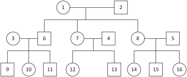
Pedigree structure for the simulation studies

Given the genotypes, we simulate the trait values using the model

$$y=0.5+0.5\text{sex}+0.05\text{age}+{\eta }_1{M}_1+{\eta }_2{M}_2+G\beta +\epsilon ,\epsilon ~N(0,{\sigma }_e^{2}I+{\sigma }_a^2\mathrm{\Phi }),$$ (13)

where M₁ and M₂ are genotype vectors for the two unobserved major genes coded as 0, 1 or 2, η₁ and η₂ are their effects on the trait, G is the genotype matrix at the m tested rare-variant sites, and β is a vector of fixed effects. Note that, in every model considered, some of the tested rare variants are non-causal. The ith tested variant being non-causal corresponds to β_i = 0 in the simulation model. The various choices of β, η₁ and η₂ used in the simulations are detailed in the following 2 subsections. We set ${\sigma }_e^2={\sigma }_a^2=1$. In each pedigree, age is a continuous covariate uniformly sampled within 1.5 years around the following mean values for individuals 1 through 16, respectively: 75, 73, 46, 46, 43, 43, 40, 40, 18, 21, 15, 17, 13, 15, 12 and 9. In the analysis of the simulated data, for all 3 tests (MONSTER, famSKAT and famBT), we calculate the test statistics using both uniform weights (i.e. $w_i=\frac{1}{m}$ for i = 1, · · ·,m) and Wu weights [Wu et al., 2011].

Assessment of Type I Error

In our type I error assessments, the phenotype is simulated under two different trait models, Models I and II. Model I, which has covariates, additive polygenic effects and independent noise, is given by Equation (13) with β = 0 and η₁ = η₂ = 0. Model II is similar to Model I with the addition of two major causal genes with effects η₁ = η₂ = 0.27. In each case, either 10 or 50 non-causal rare variant sites are simulated and are tested jointly. When Model II is used, the two major genes are assumed to be unobserved, so they are not included as covariates in the MONSTER analysis. For each scenario, 100,000 replicates are performed.

Table 1 gives the empirical type I error rates of MONSTER with nominal levels .05 and .001 for all four scenarios, where uniform weights are used. The type I error is not significantly different from the nominal using the z-test at level .01 (or using the z-test at level .05 with Bonferroni correction). Similar results were obtained using Wu weights (not shown). These results verify that MONSTER is correctly calibrated and suggest that the type I error rate is robust against deviation from the assumed null model caused by additional unobserved causal genes.

Table 1.

Empirical Type I Error of MONSTER

# Rare Variants in Test	Trait Model	Empirical Type I Error (SE) with Nominal Type I Error of
		.05	.001
50	I	.048 (.0007)	.00097 (.00010)
10	I	.049 (.0007)	.00097 (.00010)
50	II	.049 (.0007)	.00095 (.00010)
10	II	.049 (.0007)	.0011 (.00010)

Note. — Empirical type I error rates are calculated based on 100,000 replicates. None of the empirical type I error rates is significantly different from the nominal level by a z-test at level .01. Trait models I and II are described in subsection Assessment of Type I Error in Results.

Power Simulations

To compare the power of MONSTER, famSKAT and famBT, we fix the proportion of phenotypic variance attributable to the tested region and consider 6 configurations for the effects of the 50 tested rare-variant sites. These six configurations are listed as Models III-VIII in Table 2. Phenotypes are simulated according to Equation (13) with η₁ = η₂ = 0.27, corresponding to two unobserved major causal genes unlinked to the tested rare variants. Empirical power results for MONSTER, famSKAT and famBT at significance levels 10⁻⁴ and 10⁻³, based on 10,000 replicates, with uniform weights, are given in Figure 2. The power comparison was also performed with Wu weights instead of uniform weights, with qualitatively similar results (not shown). In each of Models III to V, some fraction of the variants are causal, and among the causal variants, all effects are in the same direction and are of equal magnitude. When the percentage of causal variants is low (Model III), MONSTER and famSKAT are approximately equally powerful, and are both more powerful than famBT. As the genetic effect attributable to the region (held fixed) is equally partitioned among a larger proportion of the tested variants (Models IV and V), famSKAT loses power, and the power of famBT gradually improves. In contrast, MONSTER is consistently the most powerful or has power approximately equal to the most powerful of all the tests in all three scenarios. In model VI, the causal variants have effects in opposite directions, rendering famBT powerless. In this scenario, famSKAT performs best but MONSTER also does well. In Models VII and VIII, 40% of the tested sites are causal with positive effects that can vary in size. In Model VII, the positive effects can take on two different values, while in Model VIII, every positive effect has a different value, where these are drawn from a uniform distribution. In both Models VII and VIII, MONSTER performs better than both famSKAT and famBT. Overall, MONSTER not only achieves robustness under a range of trait models, when one of famSKAT and famBT might fail, but, in addition, MONSTER actually outperforms the more powerful of famSKAT and famBT in many cases.

Table 2.

Rare-variant Effect Configurations in Power Simulations

Model	%age of Rare Variantsa with Positive/Negative/Neutral Effects	Effect Magnitudes of Causal Variantsb
III	20%/0/80%	All positive with |β| = 0.2828
IV	40%/0/60%	All positive with |β| = 0.2
V	60%/0/40%	All positive |β| = 0.1633
VI	20%/20%/60%	Half positive and half negative with |β| = 0.2
VII	40%/0/60%	All positive, half with |β| = 0.24 and half with |β| = 0.15
VIII	40%/0/60%	Effect sizes drawn i.i.d. from a uniform distribution on the interval from 0.15 to 0.2461

Note.

^aThe total number of rare variants is 50 in all models.

^bEffect sizes are determined so that approximately 1.86% of the phenotypic variance is explained by the rare variants being tested.

Figure 2.

Empirical power of MONSTER, famSKAT and famBT. Empirical power is based on 10,000 replicates for each of the six configurations of rare variant effects listed in Table 2. Standard deviations are given in parentheses.

From the simulation results, we can obtain some insight about the role of the parameter ρ in MONSTER. Figure 3 panels A-F show histograms of ρ̂, the value of ρ selected as optimal by MONSTER, for the simulations from Models III–VIII, respectively. Figure 3 panels A and D show that for Models III and VI, the ρ̂ chosen by MONSTER was usually 0. This is consistent with the power results in Figure 2 panels A and D, in which famSKAT (which is equivalent to the fixed-ρ MONSTER test with ρ = 0) has much higher power than famBT (ρ = 1), with the power of MONSTER approximately the same or slightly less than the power of famSKAT, because of the small price paid for estimating ρ. In contrast, Figure 3 panels B, C, E, and F show that for Models IV, V, VII and VIII, the ρ̂ chosen by MONSTER was usually some value strictly between 0 and 1. For scenarios in which ρ̂ is strictly between 0 and 1, it seems intuitively plausible that MONSTER could have the highest power of the 3 statistics, and, indeed, it does for Models IV, VII and VIII, while for Model V MONSTER seems to have equivalent power to that of famBT.

Figure 3.

Histograms of the optimal ρ selected by MONSTER for various simulation models. Panels A–F show the empirical distribution of the optimal ρ selected by MONSTER for Models III–VIII, respectively, where these models are given in Table 2. Each histogram is based on 10,000 replicates, and the optimal ρ is selected from {0, 0.1, …, 0.9, 1}.

It is interesting to note that ρ̂ = 1 was not chosen very often by MONSTER in any of the settings, even in Model V when famBT has equivalent power to that of MONSTER. Upon further experimentation, we found that if we increased the proportion of causal variants to 96% with effects in the same direction and of the same magnitude, then ρ̂ = 1 was the most frequently chosen value. In that case, as would be expected, famBT is more powerful than famSKAT, and the power of MONSTER is slightly lower than that of famBT. (We chose not to include this setting in Figure 2 because a proportion of causal variants of 96% seems hopelessly unrealistic.)

We also tried repeating the power studies with ρ optimized over a grid of 50 equally-spaced points on [0,1] instead of the grid of 11 equally-spaced points used for the results in Figures 2 and 3. The results change very little: the relative power change for MONSTER is uniformly within 5% across Models III to VIII. Furthermore, the empirical power based on the higher grid density is neither consistently higher nor consistently lower than that based on the lower grid density. This suggests that, at least in the context of our simulation, a denser search of ρ is not expected to improve the performance of the method.

Figure 4 shows the histogram of ρ̂ under the null hypothesis. In fact, under the null hypothesis, ρ is not identifiable, and in such a situation of low or no information in the data on a parameter, it is not surprising that MONSTER ends up choosing ρ̂ on the boundary of the parameter space, i.e. at 0 or 1, because there would tend to be very little difference among the different choices of ρ, so the algorithm would usually just drift to one end or the other of the parameter space. In order for MONSTER to prefer a ρ̂ strictly between 0 and 1, there may need to be sufficient “signal” in the data to provide information on ρ. Considered together, the results support the intuition that MONSTER can maintain high power across scenarios by either mimicking the power results of the better-performing of famSKAT and famBT in any given scenario (as in Models III and VI) or by outperforming both of them in some cases when ρ̂ is strictly between 0 and 1 (as in Models IV, VII and VIII).

Figure 4.

Histogram of optimal ρ selected by MONSTER when there is no association, based on 100,000 replicates. Simulations are based Model II with 50 tested rare variants. The optimal ρ is selected from {0, 0.1, …, 0.9, 1}.

Analysis of HDL-C Data from the Framingham Heart Study

We illustrate our approach using genotype data from the Framingham Heart Study (FHS) [Splansky et al., 2007] to investigate association with high-density lipoprotein cholesterol (HDL-C). FHS is a multi-cohort study of risk factors for cardiovascular disease, and the sample consists of unrelated individuals as well as individuals from multi-generation pedigrees. We focus on HDL-C levels in Exam 1 of Cohort 3 (third-generation cohort) of FHS. We adjust the log-transformed phenotype by age, age², sex, and log(FPG), where FPG is fasting plasma glucose. We analyze Affymetrix 500K genotype data on the third-generation cohort. We exclude from the analysis individuals who have empirical self-kinship > .525 (i.e. empirical inbreeding coefficient > .05) or whose completeness (proportion of sites for which genotype is called) ≤ 96%. In addition, we exclude a few more individuals whose empirical kinship values appear to be inconsistent with the pedigree information. Among the remaining individuals, we analyze the 3879 individuals who are both genotyped and phenotyped with no missing covariates.

We assess association with genetic variants in 14 candidate gene regions that have previously been associated or functionally linked to HDL-C (as reported in OMIM): APOA2, HADHA, HADHB, VNN1, EDN1, LPL, ABCA1, TTC39B, APOA1, SCARB1, LIPC, CETP, LIPG and PLTP. For each candidate gene region, we first extract all polymorphic sites that are on the Affymetrix 500K chip and are within 100 kb of the gene. We exclude sites that do not meet both of the following criteria: (1) call rate > 90% and (2) value of the Hardy-Weinberg χ² statistic < 100 (where this calculation assumes independent samples). We then drop from the analysis any individuals with missing genotypes at more than 10% of the remaining variants in the region. For the remaining individuals, we impute any missing genotypes using the best linear unbiased predictor [McPeek 2012].

Table 3 reports the 5 candidate gene regions out of 14 for which at least one of the three tests (MONSTER, famSKAT and famBT) gives a p-value < 10⁻², where uniform weights are used for all 3 tests. The 3 candidate genes with the smallest p-values, CETP, LPL, and LIPG, have been previously reported and replicated [Willer et al., 2008; Kathiresan et al., 2008; Aulchenko et al., 2009; Kathiresan et al., 2009]. We observe that, for 4 of the 5 candidate genes included in Table 3, famSKAT yields a smaller p-value than famBT, and MONSTER selects an optimal ρ that is zero. In that case, MONSTER would be expected to have a p-value similar to that of famSKAT but slightly larger, which is indeed the case. In addition to analyzing the data with uniform weights, we also tried using Wu weights to upweight the rarer variants, which resulted in substantially larger p-values for all tested regions by all methods (results not shown). These two observations, that the optimal ρ is usually 0 in these data and that upweighting the rarer variants results in larger p-values, might simply reflect the genetic architecture of these particular regions, but it might also be explained in part by the fact that these are Affymetrix 500K data, as opposed to sequence data. In the Affymetrix 500K data, the typed variants in each gene region are not rare, and so, a priori, are less likely to be causal, according to standard evolutionary theory [Kryukov et al., 2007]. Second, because of the limited number of typed markers within any given gene, we also consider all typed markers within 100 kb of each gene. Thus, our set of variants to be tested includes SNPs in exons as well as many possibly less relevant SNPs in untranslated segments and intergenic regions. Sequence data, on the other hand, would be more enriched for rare variants, which are more likely to be causal. Furthermore, taking advantage of the larger number of variants available in sequence data, one might be able to increase power by restricting consideration to nonsynonymous variants or functional sites predicted by bioinformatic tools, yielding an increased fraction of causal sites. Based on the simulation results, we would expect a higher proportion of causal variants in the data to lead to optimal ρ > 0 occurring more frequently. Upweighting of rarer variants might also be more effective when the data are more enriched for causal variants.

Table 3.

P-values for Association of HDL-C with 5 Candidate Gene Regions in the Framingham Heart Study Data

Gene	Chr	# SNPs in Test	p-value based on			Optimal ρ for MONSTER
			famBT	famSKAT	MONSTER
LPL	8	47	1.2 × 10−4	1.4 × 10−5	2.3 × 10−5	0
APOA1	11	32	2.4 × 10−2	4.6 × 10−3	5.7 × 10−3	0
LIPC	15	103	3.7 × 10−2	5.1 × 10−3	1.1 × 10−2	0
CETP	16	42	2.3 × 10−3	9.5 × 10−5	1.6 × 10−4	0.1
LIPG	18	49	8.7 × 10−1	3.2 × 10−6	5.3 × 10−6	0

Note. — The log-transformed phenotype is adjusted for age, age², sex and log-transformed fasting plasma glucose. Uniform weights are used. P-values in bold are those that are smaller than 10⁻³. MIM numbers of genes: LPL [MIM 609708], APOA1 [MIM 107680], LIPC [MIM 151670], CETP [MIM 118470], LIPG [MIM 603684].

It is of interest to compare the results of the multi-site tests (MONSTER, famSKAT and famBT) to single-SNP results for the same regions. To do this, we apply MASTOR [Jakobsdottir and McPeek, 2013], a recently-proposed method to test for single-SNP association with quantitative traits in samples with related individuals. The MASTOR analysis includes additive and environmental components of variance and the same covariates, same SNPs, and same set of individuals as the multi-site analyses. MASTOR can handle incomplete data, so we input only the observed genotyped data, not the imputed values. MASTOR uses the observed genotype data to provide information on the ungenotyped relatives (see Jakobsdottir and McPeek [2013] for details). For each region, Table 4 gives the minimum p-value obtained by MASTOR as well as the Bonferroni-corrected p-value. For all 5 candidate genes except CETP, the p-values of MONSTER and famSKAT are smaller than the Bonferroni-corrected p-value of MASTOR. For LIPG, even the minimum p-value from MASTOR is greater than the multi-site p-values of MONSTER and famSKAT. To better understand these results, we examine in more detail the association signals of individuals SNPs for these genes. For LIPG, of 49 tested SNPs, the 9 SNPs that have p-value < .001 are spread across multiple linkage disequilibrium blocks and have comparable p-values. In that case, it is reasonable to expect that a multi-site test would gain an advantage over a single-site test by aggregating information across sites to boost power. In contrast, the association signal at CETP is dominated by a single SNP, rs9989419 (p = 1.6 × 10⁻⁸), with two much more weakly-associated SNPs (p = 5.5 × 10⁻⁴ and p = 6.9 × 10⁻³), and with all other SNPs having p-value > 0.01. When most of the association signal is attributable to a single SNP, it is reasonable to expect a single-SNP test to outperform multi-site tests.

Table 4.

Single-Site Association Results for HDL-C with SNPS in 5 Candidate Gene Regions in the Framingham Heart Study Data

Gene	Minimum P-value	P-value after Bonferroni Correction	Most Significant SNP
LPL	1.4 × 10−6	6.8 × 10−5	rs17489282
APOA1	9.0 × 10−4	2.9 × 10−2	rs17440396
LIPC	2.5 × 10−3	2.6 × 10−1	rs4775041
CETP	1.6 × 10−8	6.6 × 10−7	rs9989419
LIPG	1.4 × 10−5	7.0 × 10−4	rs7240405

Note. — P-values are based on the single-variant association test, MASTOR [Jakobsdottir and McPeek, 2013]. P-values in bold are those that are < 10⁻³.

Computation Time

The main computational burden of MONSTER comes from the eigenvalue decomposition of the kinship matrix, which is needed for calculation of the p-value. When the sample consists of multiple independent families, the block-diagonal structure of the kinship matrix allows the decomposition to be performed separately for each family, which can substantially reduce the computation time. The eigenvalue decomposition generally needs to be performed only once for each tested region. Furthermore, if the tests corresponding to different regions are all based on the same set of typed individuals (i.e., the set of individuals with missing data does not vary across regions), then the decomposition need only be performed once overall, with the same decomposition results used for every region.

We implement MONSTER in a freely-downloadable software package that uses the above-described speed-ups when appropriate. We give some example run times of MONSTER for analysis of the FHS HDL-C data discussed in the previous subsection. This data set contains 3879 individuals from 768 families that range in size from 1 to 174 individuals. Using a single processor on a shared machine with 4 core Intel Xeon 3.16GHz CPUs and 32GB RAM, MONSTER took 2.1 seconds to analyze a genetic region of 50 variants. Doubling the number of tested variants in the region to 100 only increased the run time to 2.6 seconds. Extrapolating to an analysis of 20,000 different gene regions with 100 variants included in each test, and assuming that different regions had different sets of individuals in their tests (so that the eigen-decomposition would have to be calculated separately for every region), MONSTER would require approximately 14.4 hours for the entire analysis. This time would be substantially reduced if the same set of individuals were included in all tests. These results demonstrate that MONSTER is computationally feasible for large-scale studies.

Discussion

The presence of related individuals in high-throughput sequencing studies is common and can yield advantages such as (i) enhanced ability to detect sequencing error, (ii) more efficient use of available data through accurate imputation of relatives’ sequence data, and (iii) the opportunity to observe multiple copies of very rare variants, which can improve power to detect association. We have developed MONSTER, a method for detecting association between a set of rare variants and a quantitative trait in samples that contain related individuals. MONSTER is based on a mixed-effects model that includes additive and environmental components of variance and adjustment for covariates. It can handle essentially arbitrary combinations of related and unrelated individuals, including small outbred pedigrees and unrelated individuals, as well as large, complex inbred pedigrees. In simulation studies, we demonstrate that MONSTER is a powerful and robust approach that performs well in a wide range of scenarios. We illustrate the use of MONSTER with an application to candidate gene association analysis of HDL-C in the FHS, in which we replicate association with 3 genes.

MONSTER can be viewed as an extension of the SKAT-O method to samples with related individuals. The MONSTER test statistic is also shown to be a convex combination of the famSKAT and famBT test statistics, with an adaptively-determined parameter, ρ, that controls the relative weights of the two statistics. The famSKAT and famBT tests tend to be powerful in different scenarios. FamBT tends to have higher power than famSKAT when a large fraction of tested variants are causal with effects in the same direction, while the reverse tends to be true when (i) the fraction of tested variants that are causal is low, (ii) there is a mixture of protective and deleterious variants or (iii) effect sizes vary substantially across tested variants. In a given simulation scenario, MONSTER tends to either mimic the performance of the better-performing of famSKAT and famBT (with optimal ρ chosen as either 0 or 1) or to outperform both statistics, which can happen when the optimal ρ is chosen strictly between 0 and 1. This robustness of power to the underlying modeling assumptions can be very desirable in practice, as the true biological mechanism and genetic architecture is usually unknown a priori and can be expected to vary across genes and traits.

In the simulations and data analysis, we apply MONSTER with the nuisance parameter ρ optimized over a grid of 11 values in [0,1]. In the simulations, we found that searching over a denser grid of 50 values did not improve the performance. The effect of grid density is presumably related to the amount of information the data contain about the nuisance parameter ρ, which is in turn related to sample size. Larger samples tend to offer more information on ρ, resulting in a more concentrated distribution of the chosen ρ̂ value. When using MONSTER on small samples, one might consider optimizing ρ over a coarser grid on [0, 1] to reduce the price paid by estimating ρ. This is advantageous compared to simply using either famSKAT or famBT, because it is usually unclear a priori which of them would be more powerful, and because an intermediate ρ value could potentially improve power. For larger samples, one could in principle search over a denser grid of ρ, though in the context of our simulations, increasing the density of the grid does not seem to yield a power gain.

MONSTER assumes known pedigree information, or at least, known kinship. It would be possible to extend the method to allow for (i) additional population structure or kinship beyond that explained by the known pedigree information or (ii) completely unknown kinship. To extend MONSTER to allow (ii), we could replace the pedigree-based kinship matrix Φ with an empirical kinship matrix, Φ calculated based on genome-wide data, as is done in, for example, ROADTRIPS [Thornton and McPeek, 2010] or EMMAX [Kang et al., 2010]. A simple approach to allow (i) would be to use the modeling assumption

$$\mathit{Var}(y\mid \beta ,X,G)={\sigma }_e^{2}I+{\sigma }_a^2\mathrm{\Phi }+{\sigma }_s^2\widehat{\mathrm{\Phi }},$$ (14)

with the additional unknown variance component, ${\sigma }_s^2$, included to account for population structure or kinship beyond that explained by the known pedigree information (R. Cheng, C. C. Parker, M. Abney, A. A. Palmer, personal communication). Another method to control for population stratification would be to include, as covariates, ancestry proportions for the individuals, which can be estimated using existing software packages [Tang et al., 2005; Alexander et al., 2009].

In addition to an additive polygenic variance component, it may sometimes be useful to include a dominance variance component, ${\sigma }_d^2$. This could be done by changing the model for the conditional variance of the trait to

$$\mathit{Var}(y\mid \beta ,X,G)={\sigma }_e^{2}I+{\sigma }_a^2\mathrm{\Phi }+{\sigma }_d^2{\mathrm{\Delta }}_7,$$ (15)

where Δ₇ is a matrix whose (i, j)th component, ${\mathrm{\Delta }}_7^{ij}$, is the 7th condensed identity coefficient between individuals i and j [Abney et al., 2000]. When i and j are outbred, ${\mathrm{\Delta }}_7^{ij}$ is the probability that i and j share two alleles identical by descent. For inclusion of a dominance variance component to provide additional power, it would presumably be necessary that (i) the trait have a strong dominance component and that (ii) the composition of the sample be such that many pairs of the sampled individuals would have a nonnegligible probability of sharing two alleles identical by descent (e.g., MZ twins, sib pairs, and double first cousins).

MONSTER imposes a common correlation coefficient ρ for the random effects of all pairs of tested variants. This is a reasonable choice when there is little prior functionality information on the variants. If additional relevant prior information were available, MONSTER could be extended to allow for a different correlation structure among the variant effects. For example, a pair of variants that code the same protein domain could be given a larger correlation coefficient than a pair that do not. Additional nuisance parameters could also be included in the correlation matrix to reflect a more structured relationship among the tested sites.

References

- Abney M, McPeek MS, Ober C. Estimation of variance components of quantitative traits in inbred populations. Am J Epidemiol. 2000;66:629–650. doi: 10.1086/302759. [DOI] [PMC free article] [PubMed] [Google Scholar]
- Alexander DH, Novembre J, Lange K. Fast model-based estimation of ancestry in unrelated individuals. Genome Res. 2009;19:1655–1664. doi: 10.1101/gr.094052.109. [DOI] [PMC free article] [PubMed] [Google Scholar]
- Aulchenko YS, Ripatti S, Lindqvist I, Boomsma D, Heid IM, Pramstaller PP, Penninx BWJH, Janssens ACJW, Wilson JF, Spector T, et al. Loci in uencing lipid levels and coronary heart disease risk in 16 European population cohorts. Nat Genet. 2009;41:47–55. doi: 10.1038/ng.269. [DOI] [PMC free article] [PubMed] [Google Scholar]
- Chen H, Meigs JB, Dupuis J. Sequence kernel association test for quantitative traits in family samples. Genet Epidemiol. 2013;37:196–204. doi: 10.1002/gepi.21703. [DOI] [PMC free article] [PubMed] [Google Scholar]
- Eichler EE, Flint J, Gibson G, Kong A, Leal SM, Moore JH, Nadeau JH. Missing heritability and strategies for finding the underlying causes of complex disease. Nat Rev Genet. 2010;11:446–450. doi: 10.1038/nrg2809. [DOI] [PMC free article] [PubMed] [Google Scholar]
- Goeman JJ, van de Geer SA, van Houwelingen HC. Testing against a high dimensional alternative. J R Statist Soc B. 2006;68:477–493. [Google Scholar]
- Ionita-Laza I, Lee S, Makarov V, Buxbaum JD, Lin X. Family-based association tests for sequence data, and comparisons with population-based association tests. Eur J Hum Genet. 2013 doi: 10.1038/ejhg.2012.308. In press. [DOI] [PMC free article] [PubMed] [Google Scholar]
- Jakobsdottir J, McPeek MS. MASTOR: Mixed-model association mapping of quantitative traits in samples with related individuals. Am J Hum Genet. 2013;92:652–666. doi: 10.1016/j.ajhg.2013.03.014. [DOI] [PMC free article] [PubMed] [Google Scholar]
- Kang HM, Sul JH, Service SK, Zaitlen NA, Kong SY, Freimer NB, Sabatti C, Eskin E. Variance component model to account for sample structure in genome-wide association studies. Nat Genet. 2010;42:348–54. doi: 10.1038/ng.548. [DOI] [PMC free article] [PubMed] [Google Scholar]
- Kathiresan S, Melander O, Guiducci C, Surti A, Burtt NP, Rieder MJ, Cooper GM, Roos C, Voight BF, Havulinna AS, et al. Six new loci associated with blood low-density lipoprotein cholesterol, high-density lipoprotein cholesterol or triglycerides in humans. Nat Genet. 2008;40:189–197. doi: 10.1038/ng.75. [DOI] [PMC free article] [PubMed] [Google Scholar]
- Kathiresan S, Willer CJ, Peloso GM, Demissie S, Musunuru K, Schedt EE, Kaplan L, Bennett D, Li Y, Tanaka T, et al. Common variants at 30 loci contribute to polygenic dyslipidemia. Nat Genet. 2009;41:56–65. doi: 10.1038/ng.291. [DOI] [PMC free article] [PubMed] [Google Scholar]
- Kazma R, Bailey JN. Population-based and family-based designs to analyze rare variants in complex diseases. Genet Epidemiol. 2011;35(Suppl 1):S41–S47. doi: 10.1002/gepi.20648. [DOI] [PMC free article] [PubMed] [Google Scholar]
- Kryukov GV, Pennacchio LA, Sunyaev SR. Most rare missense alleles are deleterious in humans: implications for complex disease and association studies. Am J Hum Genet. 2007;80:727–739. doi: 10.1086/513473. [DOI] [PMC free article] [PubMed] [Google Scholar]
- Lee S, Wu MC, Lin X. Optimal tests for rare variant effects in sequencing association studies. Biostatistics. 2012;13:762–775. doi: 10.1093/biostatistics/kxs014. [DOI] [PMC free article] [PubMed] [Google Scholar]
- Li B, Leal SM. Methods for detecting associations with rare variants for common diseases: application to analysis of sequence data. Am J Hum Genet. 2008;83:311–321. doi: 10.1016/j.ajhg.2008.06.024. [DOI] [PMC free article] [PubMed] [Google Scholar]
- Liu H, Tang Y, Zhang HH. A new chi-square approximation to the distribution of non-negative definite quadratic forms in non-central normal variables. Comput Stat Data An. 2009;53:853–856. [Google Scholar]
- Madsen BE, Browning SR. A groupwise association test for rare mutations using a weighted sum statistic. PLoS Genet. 2009;5:e1000384. doi: 10.1371/journal.pgen.1000384. [DOI] [PMC free article] [PubMed] [Google Scholar]
- Manolio TA, Collins FS, Cox NJ, Goldstein DB, Hindorff LA, Hunter DJ, McCarthy MI, Ramos EM, Cardon LR, Chakravarti A, et al. Finding the missing heritability of complex diseases. Nature. 2009;461:747–753. doi: 10.1038/nature08494. [DOI] [PMC free article] [PubMed] [Google Scholar]
- McPeek MS. BLUP Genotype Imputation for case-control association testing with related individuals and missing data. J Comput Biol. 2012;19:756–765. doi: 10.1089/cmb.2012.0024. [DOI] [PMC free article] [PubMed] [Google Scholar]
- Morgenthaler S, Thilly WG. A strategy to discover genes that carry multi-allelic or mono-allelic risk for common diseases: a cohort allelic sums test (CAST) Mutat Res. 2007;615:28–56. doi: 10.1016/j.mrfmmm.2006.09.003. [DOI] [PubMed] [Google Scholar]
- Neale BM, Rivas MA, Voight BF, Altshuler D, Devlin B, Orho-Melander M, Kathiresan S, Purcell SM, Roeder K, Daly MJ. Testing for an unusual distribution of rare variants. PLoS Genet. 2011;7:e1001322. doi: 10.1371/journal.pgen.1001322. [DOI] [PMC free article] [PubMed] [Google Scholar]
- Price AL, Kryukov GV, de Bakker PI, Purcell SM, Staples J, Wei LJ, Sunyaev SR. Pooled association tests for rare variants in exon-resequencing studies. Am J Hum Genet. 2010;86:832–838. doi: 10.1016/j.ajhg.2010.04.005. [DOI] [PMC free article] [PubMed] [Google Scholar]
- Roach JC, Glusman G, Smit AFA, Huff CD, Hubley R, Shannon PT, Rowen L, Pant KP, Goodman N, Bamshad M, et al. Analysis of genetic inheritance in a family quartet by whole-genome sequencing. Science. 2010;328:636–639. doi: 10.1126/science.1186802. [DOI] [PMC free article] [PubMed] [Google Scholar]
- Schaid DJ, McDonnell SK, Sinnwell JP, Thibodeau SM. Multiple genetic variant association testing by collapsing and kernel methods with pedigree or population structured data. Genet Epidemiol. 2013;37:409–418. doi: 10.1002/gepi.21727. [DOI] [PMC free article] [PubMed] [Google Scholar]
- Schifano ED, Epstein MP, Bielak LF, Jhun MA, Kardia SLR, Peyser PA, Lin X. SNP set association analysis for familial data. Genet Epidemiol. 2012;36:797–810. doi: 10.1002/gepi.21676. [DOI] [PMC free article] [PubMed] [Google Scholar]
- Splansky GL, Corey D, Yang Q, Atwood L, Cupples LA, Benjamin EJ, D’Agostino RB, Sr, Fox CS, Larson MG, Murabito JM, et al. The third generation cohort of the national heart, lung, and blood institute’s Framingham heart study: design, recruitment, and initial examination. Am J Epidemiol. 2007;165:1328–1335. doi: 10.1093/aje/kwm021. [DOI] [PubMed] [Google Scholar]
- Tang H, Peng J, Wang P, Risch NJ. Estimation of individual admixture: analytical and study design considerations. Genet Epidemiol. 2005;28:289–301. doi: 10.1002/gepi.20064. [DOI] [PubMed] [Google Scholar]
- Thornton T, McPeek MS. ROADTRIPS: Case-control association testing with partially or completely unknown population and pedigree structure. Am J Hum Genet. 2010;86:172–184. doi: 10.1016/j.ajhg.2010.01.001. [DOI] [PMC free article] [PubMed] [Google Scholar]
- Uricchio LH, Chong JX, Ross KD, Ober C, Nicolae DL. Accurate imputation of rare and common variants in a founder population from a small number of sequenced individuals. Genet Epidemiol. 2012;36:312–319. doi: 10.1002/gepi.21623. [DOI] [PMC free article] [PubMed] [Google Scholar]
- Wang Y, Chen YH, Yang Q. Joint rare variant association test of the average and individual effects for sequencing studies. PLoS One. 2012;7:e32485. doi: 10.1371/journal.pone.0032485. [DOI] [PMC free article] [PubMed] [Google Scholar]
- Willer CJ, Sanna S, Jackson AU, Scuteri A, Bonnycastle LL, Clarke R, Heath SC, Timpson NJ, Najjar SS, Stringham HM, et al. Newly identified loci that in uence lipid concentrations and risk of coronary artery disease. Nat Genet. 2008;40:161–169. doi: 10.1038/ng.76. [DOI] [PMC free article] [PubMed] [Google Scholar]
- Wu MC, Lee S, Cai T, Li Y, Boehnke M, Lin X. Rare-variant association testing for sequencing data with the sequence kernel association test. Am J Hum Genet. 2011;89:82–93. doi: 10.1016/j.ajhg.2011.05.029. [DOI] [PMC free article] [PubMed] [Google Scholar]
- Zhou B, Whittemore AS. Improving sequence-based genotype calls with linkage disequilibrium and pedigree information. Ann Appl Stat. 2012;6:457–475. [Google Scholar]