HYPOTHESIS TESTING FOR HIGH-DIMENSIONAL SPARSE BINARY REGRESSION

Abstract

In this paper, we study the detection boundary for minimax hypothesis testing in the context of high-dimensional, sparse binary regression models. Motivated by genetic sequencing association studies for rare variant effects, we investigate the complexity of the hypothesis testing problem when the design matrix is sparse. We observe a new phenomenon in the behavior of detection boundary which does not occur in the case of Gaussian linear regression. We derive the detection boundary as a function of two components: a design matrix sparsity index and signal strength, each of which is a function of the sparsity of the alternative. For any alternative, if the design matrix sparsity index is too high, any test is asymptotically powerless irrespective of the magnitude of signal strength. For binary design matrices with the sparsity index that is not too high, our results are parallel to those in the Gaussian case. In this context, we derive detection boundaries for both dense and sparse regimes. For the dense regime, we show that the generalized likelihood ratio is rate optimal; for the sparse regime, we propose an extended Higher Criticism Test and show it is rate optimal and sharp. We illustrate the finite sample properties of the theoretical results using simulation studies.

1. Introduction

The problem of testing for the association between a set of covariates and a response is of fundamental statistical interest. In the context of testing for a linear relationship of covariates with a continuous response, R. A. Fisher introduced analysis of variance (ANOVA) in the 1920s, which is still widely used in the present day. In recent years, finding the detection boundary of various testing problems has gained substantial popularity. A fruitful way of finding the detection boundary is to study the minimax error of testing and obtain a threshold of signal strength under which all testing procedures in the concerned problem are useless. For Gaussian linear models, this has been extensively studied by Arias-Castro, Candès and Plan (2011) and Ingster, Tsybakov and Verzelen (2010); these works were inspired by the previous work on hypothesis testing in various contexts, such as sparse normal mixtures [Donoho and Jin (2004), Cai, Jeng and Jin (2011)], Gaussian sequence models [Ingster and Suslina (2003)] and correlated multivariate normal problems [Hall and Jin (2010)]. However, very little work has been done on detection boundaries in generalized linear models for discrete outcomes.

In this paper, we study the detection boundary for hypothesis testing in the context of high-dimensional, sparse binary regression models. Motivated by case–control sequencing association studies for detecting the effects of rare variants on disease risk [Tang et al. (2014), Lee et al. (2014)], we are interested in the complexity of the hypothesis testing problem when the design matrix is sparse. Specifically, sequencing studies allow sequencing massive genetic variants in candidate genes or across the whole genome. A rapidly increasing number of sequencing association studies have been conducted, such as the 1000 Genome Project [1000 Genomes Project Consortium (2012)] and the NHLBI Exome Sequencing Project [Fu et al. (2013)]. It is of substantial interest to study rare variant effects on diseases case–control candidate gene and whole genome sequencing association studies. A major challenge in analysis of sequencing data is that a vast majority of variants across the genome are rare variants [1000 Genomes Project Consortium (2012) (Figure 2b), Fu et al. (2013) (Figure 1a), Nelson et al. (2012) (Figure 1c)]. For a review of analysis of data of sequencing association studies, see Lee et al. (2014).

Fig. 2.

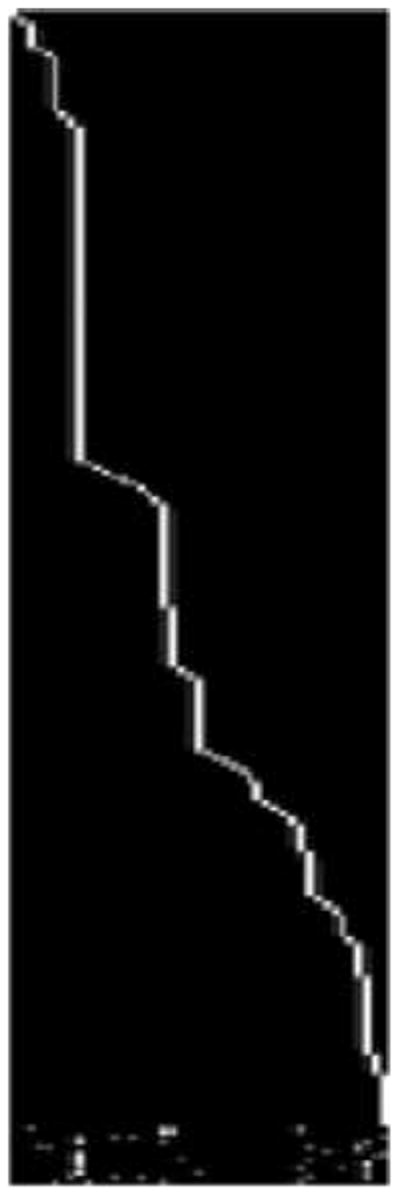
Heat map of the genotype matrix X of the Dallas Heart study data after a suitable rearrangement of subject indices, after removing the single common variant. The nonzero entries of the genotype matrix that represent mutations are colored white, while the zero entries that represent no mutation are colored in black.

Fig. 1.

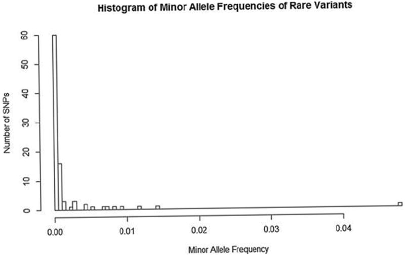
The histogram of minor allele frequencies of uncommon/rare variants (MAF ≤ 5%) in the Dallas Heart study data.

For example, in the Dallas Heart candidate gene sequencing study [Victor et al. (2004)], 3476 individuals were sequenced in the region consisting of three genes ANGPTL3, ANGPTL4 and ANGPTL5. The goal of study was to test the effects of these genes on the risk of hypertriglyceridemia. A total of 93 genetic variants were observed in these genes. Each variant took values 0, 1, 2, which represents the number of minor alleles in a genetic variant. About half of the variants were singletons, that is, they were observed in only one person; 92 variants have the minor allele frequencies < 5%. The design matrix is hence very sparse, with a vast majority of its columns having <5% nonzero values (1 or 2), and the proportion of total nonzero elements in the design matrix being <2.5%. It is expected only a small number of variants might be associated with hypertriglyceridemia. The presence of the sparse design matrix and sparse signals for binary outcomes results in substantial challenges in testing the association of these genes and hypertriglyceridemia. Figure 1 provides the histogram of rare variants with minor allele frequencies less than 5%.

Suppose there are n samples of binary outcomes, p covariates for each. Consider a binary regression model linking the outcomes to the covariates. We are interested in testing a global null hypothesis that the regression coefficients are all zero and the alternative is sparse with k signals, where k = p^1−α and α ∈ [0, 1]. For binary regression models, we observe a new phenomenon in the behavior of detection boundaries which does not occur in the Gaussian framework, as explained below.

The main contribution of our paper is to derive the detection boundary for binary regression models as a function of two components: a design matrix sparsity index and signal strength, each of which is a function of the sparsity of the alternative, that is, α. Throughout the paper, we will call the first component as “design matrix sparsity index.” This is unlike the results in Gaussian linear regression which has a one component detection boundary, namely the necessary signal strength. In the Gaussian linear model framework, Arias-Castro, Candès and Plan (2011) and Ingster, Tsybakov and Verzelen (2010) show that if the design matrix satisfies certain “low coherence conditions,” then it is possible to detect the presence of a signal in a global sense, provided the signal strength exceeds a certain threshold. In contrast, our results suggest that for binary regression problems, the difficulty of the problem is also determined by the design matrix sparsity index. In this paper, we explore two key implications of this phenomenon which are outlined below.

First, if the design matrix sparsity index is too high, we show that no signal can be detected irrespective of its strength. In Section 3, we provide sufficient conditions on the design matrix sparsity index which yield such nondetectability problems. Such conditions on the design matrix sparsity index corresponds to the first component of the detection boundary. Plan and Vershynin (2013a, 2013b) discussed a difficulty in inference similar to that of ours, for design matrices with binary entries in the context of 1-bit compressive sensing and sparse logistic models. Our results in Section 3 pertain to sparse design matrices with arbitrary entries, which are not necessarily orthogonal. We give a few examples of design matrices which satisfy our criteria for nondetectability. These include block diagonal matrices and banded matrices.

Second, for design matrices with binary entries and with low correlation among the columns, we are able to characterize both components of the detection boundary. In particular, if the design matrix sparsity index, the first component of the detection boundary, is above a specified threshold, no signal is detectable irrespective of strength. Once the design matrix sparsity index is below the same threshold, we also obtain the optimal thresholds with respect to the second component of the detection boundary, that is, the minimum signal strength required for successful detection. In this regime, our results parallel the theory of detection boundary in Gaussian linear regression. We also provide relevant tests to attain the optimal detection boundaries. In the sparse regime ( $\alpha >\frac{1}{2}$), our results are sharp and rate adaptive in terms of the signal strength component of the detection boundary. Moreover, we observe a phase transition in both components of the detection boundary depending on the sparsity (α) of the alternative. To the best of our knowledge, this is the first work optimally characterizing a two component detection boundary in global testing problems against sparse alternatives in binary regression.

To illustrate further, we contrast our results with the existing literature. In the case of a balanced one-way ANOVA type design matrix with each treatment having r independent replicates, for Gaussian linear models, Arias-Castro, Candès and Plan (2011) show that the detection boundary is given by $O(\frac{p^{1/4}}{\sqrt{\mathit{kr}}})$ in the dense regime ( $\alpha <\frac{1}{2}$) and equals $\sqrt{\frac{2{\rho }_{\mathrm{linear}}^{\ast }(\alpha )\log (p)}{r}}$ in the sparse regime $\alpha >\frac{1}{2}$, where

$${\rho }_{\mathrm{linear}}^{\ast }(\alpha )=\{\begin{array}{ll}\alpha -\frac{1}{2},& \mathrm{if}\frac{1}{2}<\alpha <\frac{3}{4},\\ {(1-\sqrt{1-\alpha })}^2,& \mathrm{if}\alpha \ge \frac{3}{4}\end{array}$$ (1.1)

and ${\rho }_{\mathrm{linear}}^{\ast }(\alpha )$ matches the detection boundary in Donoho and Jin (2004) in the normal mixture problem. For given sparsity of the alternative, the detection boundary depends a single function of r.

For binary regression, we show that the detection boundary is drastically different and depends on two functions of r: a design matrix sparsity index and signal strength under the alternative hypothesis for a given regime. In particular, define the design matrix sparsity index of a design matrix as 1/r. For r = 1, every test is powerless irrespective of the signal sparsity and the signal strength under the alternative hypothesis. When r > 1, the behavior of the detection boundary can be categorized into three situations. In the dense regime where r > 1 and $\alpha \le \frac{1}{2}$, the detection boundary matches that of the Gaussian case up to rates and the usual Generalized Likelihood Ratio Test achieves the detection boundary. In the sparse regime, that is, when $\alpha >\frac{1}{2}$, the detection boundary behaves differently for r ≪ log(p) and r ≫ log(p). For $\alpha >\frac{1}{2}$ and r ≪ log(p), a new phenomenon that does not exist in the Gaussian case arises: all tests are asymptotically powerless irrespective of how strong the signal strength is in the alternative. For $\alpha >\frac{1}{2}$ and r ≫ log(p), our results are identical to the Gaussian case, up to a constant factor accounting for the Fisher information. In this regime, we construct a version of the Higher Criticism Test and show that this test achieves the lower bound. We use the strong embedding theorem [Komlós, Major and Tusnády (1975)] to obtain sharp detection boundary. Noting that this problem can also be cast as a test of homogeneity among p binomial populations with contamination in k of them. Hence, roughly speaking, the two component detection boundary in this binary problem setting equals [1, $O(\frac{p^{1/4}}{\sqrt{\mathit{kr}}})$) in the dense regime and ( $O(\frac{1}{\log (p)})$, $O(\sqrt{\frac{\log (p)}{r}})$] in the sparse regime, where the first component represents the design matrix sparsity index, which is of the order of 1/r, and the second component indicates the order of signal strength. Successful detection requires both components to be above the component-specific detection boundaries.

Borrowing ideas from orthogonal designs, we further obtain analogous results for general binary design matrices which are sparse and have weak correlation among columns, mimicking design matrices often observed in sequencing association studies. For such general binary designs, we are able to completely characterize the two component detection boundary in both dense and sparse regimes. Our versions of Generalized Likelihood Ratio Test and the Higher Criticism Test continue to attain the optimal detection boundaries in dense and sparse regimes, respectively. Similar to orthogonal designs, our results are sharp in the sparse regime and we once again obtain optimal phase transition in the two component detection boundary depending on the sparsity (α) of the alternative. Our results show that under certain low correlation structures, the problem essentially behaves as an orthogonal problem.

The rest of the paper is organized as follows. We first formally introduce the model in Section 2 and discuss general strategies. Here, we also provide a set of notation to be used throughout the paper. In Section 3, we study the nondetectability for sparse design matrices with arbitrary entries. In Section 4, we formally introduce a class of designs for which we derive the sharp detection boundaries, namely, one-way ANOVA designs and weakly correlated binary designs. Section 5 introduces the Generalized Likelihood Ratio Test (GLRT) and the Higher Criticism Test in our designs, which will be used in subsequent sections to attain the sharp detection boundaries in two different regimes of sparsity. In Section 6, we first analyze the oneway ANOVA designs and derive the sharp detection boundary in different sparsity regimes. In Section 7, we derive the sharp detection boundary in different sparsity regimes for weakly correlated binary designs. Section 8 presents simulation studies which validate our theoretical results. Finally, we collect all the technical proofs in the supplementary material [Mukherjee, Pillai and Lin (2014)].

2. Preliminaries

Suppose there are n binary observations y_i ∈ {0, 1}, for 1 ≤ i ≤ n, with covariates x_i = (x_i1, …, x_ip)^t. The design matrix with rows ${\mathbf{x}}_i^t$ is denoted by X. Set y = (y₁, y₂, …, y_n)^t. The conditional distribution of y_i given x_i is given by

$$\mathbb{P}(y_i=1\mid {\mathbf{x}}_i,\mathit{\beta })=\theta ({\mathbf{x}}_i^t\mathit{\beta }),$$ (2.1)

where β = (β₁, …, β_p)^t ∈ ℝ^p is an unknown p-dimensional vector of regression coefficients. Henceforth, we will assume that θ is an arbitrary distribution function that is symmetric around 0, that is,

$$\theta (z)+\theta (-z)=1\mathrm{for\; all}z\in ℝ.$$ (2.2)

For some of the results, we will also require certain smoothness assumptions on θ(·) which we will state when and where required. Examples of such θ(·) include logistic and normal distributions which, respectively, correspond to logistic and probit regression models.

Let $M(\mathit{\beta })={\sum }_{j=1}^{p}I({\beta }_j\ne 0)$ and let $R_k^p=\{\mathit{\beta }\in {ℝ}^p:M(\mathit{\beta })=k\}$. For some A > 0, we are interested in testing the global null hypothesis

$$H_0:\mathit{\beta }=0\mathrm{vs}{H}_1:\mathit{\beta }\in {\mathrm{\Theta }}_k^A=\left\{\mathit{\beta }\in \underset{k^{\prime }\ge k}{\cup }{R}_{k^{\prime }}^p:\min \{|{\beta }_j|:{\beta }_j\ne 0\}\ge A\right\}.$$ (2.3)

Set k = p^1−α with α ∈ (0, 1]. We note that these types of alternatives have been considered by Arias-Castro, Candès and Plan (2011), referred to as the “Sparse Fixed Effects Model” or SFEM. In particular, under the alternative, β has at least k nonzero coefficients exceeding A in absolute values. Alternatives corresponding to $\alpha \le \frac{1}{2}$ belong to the dense regime and those corresponding to $\alpha >\frac{1}{2}$ belong to the sparse regime. We will denote by π a prior distribution on ${\mathrm{\Theta }}_k^A\subset {ℝ}^p$. Throughout we will refer to A as the signal strength corresponding to the alternative in equation (2.3).

We first recall a few familiar concepts from statistical decision theory. Let a test be a measurable function of the data taking values in {0, 1}. The Bayes risk of a test T = T(X, y) for testing H₀ : β = 0 versus H₁ : β ~ π when H₀ and H₁ occur with the same probability, is defined as the sum of its probability of type I error (false positives) and its average probability of type II error (missed detection):

$${\mathrm{Risk}}_{\pi }(\mathrm{T}):={\mathbb{P}}_0(\mathrm{T}=1)+\pi [{\mathbb{P}}_{\mathit{\beta }}(\mathrm{T}=0)],$$

where ℙ_βdenotes the probability distribution of y under model (2.1) and π[·] is the expectation with respect to the prior π. We study the asymptotic properties of the binary regression model (2.1) in the high-dimensional regime, that is, with p → ∞ and n = n(p) → ∞ and a sequence of priors {π_p}. Adopting the terminology from Arias-Castro, Candès and Plan (2011), we say that a sequence of tests {T_n,p} is asymptotically powerful if lim_p→∞ Risk_πp(T_n,p) = 0, and it is asymptotically powerless if lim inf_p→∞ Risk_πp(T_n,p) ≥ 1. When no prior is specified, the risk is understood to be the worst case risk or the minimax risk defined as

$$\mathrm{Risk}(\mathrm{T}):={\mathbb{P}}_0(\mathrm{T}=1)+\underset{\mathit{\beta }\in {\mathrm{\Theta }}_k^A}{\max }[{\mathbb{P}}_{\mathit{\beta }}(\mathrm{T}=0)].$$

The detection boundary of the testing problem (2.3) is the demarcation of signal strength A which determines whether all tests are asymptotically powerless (we call this lower bound of the problem) or there exists some test which is asymptotically powerful (we call this the upper bound of the problem).

To understand the minimax risk, set

$$d(P_0,P_1)=\inf \{{|P-Q|}_1:P\in P_0,Q\in P_1\},$$

where P₀, P₁ are two families of probability measures and |P – Q|₁ = sup_B |P(A) – Q(A)|, with B being a Borel set in ℝⁿ, denotes the total-variation norm. Then for any test T, we have [Wald (1950)]

$$\mathrm{Risk}(\mathrm{T})\ge 1-\frac{1}{2}d({\mathbb{P}}_0,{\mathrm{conv}}_{\mathit{\beta }\in {\mathrm{\Theta }}_k^A}({\mathbb{P}}_{\mathit{\beta }})),$$

where conv denotes the convex hull. However, $d({\mathbb{P}}_0,{\mathrm{conv}}_{\mathit{\beta }\in {\mathrm{\Theta }}_k^A}({\mathbb{P}}_{\mathit{\beta }}))$ is difficult to calculate. But it is easy to see that for any test T and any prior π, one has Risk(T) ≥ Risk_π(T). So in order to prove that a sequence of tests is asymptotically powerful, it suffices to bound from above the worst-case risk Risk(T). Similarly, in order to show that all tests are asymptotically powerless, it suffices to work with an appropriate prior to make calculations easier and bound the corresponding risk from below for any test T.

It is worth noting that, for any prior π on the set of k-sparse vectors in ℝ^p and for any test T, we have

$${\mathrm{Risk}}_{\pi }(\mathrm{T})\ge 1-\frac{1}{2}{\mathrm{E}}_0|L_{\pi }-1|\ge 1-\frac{1}{2}\sqrt{{\mathrm{E}}_0(L_{\pi }^2)-1},$$

where L_π is the π-integrated likelihood ratio and E₀ denotes the expectation under H₀. For the model (2.1), we have

$$L_{\pi }=2^n\mathit{\int }\prod _{i=1}^n{\left(\frac{\theta ({\mathrm{x}}_i^t\mathit{\beta })}{\theta (-{\mathbf{x}}_i^t\mathit{\beta })}\right)}^{y_i}\theta (-{\mathbf{x}}_i^t\mathit{\beta })\mathit{d\pi }(\mathit{\beta }).$$ (2.4)

Hence, in order to assess the lower bound for the risk, it suffices to bound from above ${\mathrm{E}}_0(L_{\pi }^2)$. By Fubini’s theorem, for fixed design matrix X, we have

$$\begin{array}{l}{\mathrm{E}}_0(L_{\pi }^2)\\ =2^n\mathit{\int }\mathit{\int }\prod _{j=1}^n[\theta ({\mathbf{x}}_i^t\mathit{\beta })\theta ({\mathbf{x}}_i^t{\mathit{\beta }}^{\prime })+\theta (-{\mathbf{x}}_i^t\mathit{\beta })\theta (-{\mathbf{x}}_i^t{\mathit{\beta }}^{\prime })]\mathit{d\pi }(\mathit{\beta })\mathit{d\pi }({\mathit{\beta }}^{\prime }),\end{array}$$ (2.5)

where β, β′ ~ π are independent. In the rest of the paper, all of our analysis is based on studying ${\mathrm{E}}_0(L_{\mathrm{\pi }}^2)$ carefully for the prior distribution π chosen below.

In the context of finding an appropriate test matching the lower bound, by the Neyman–Pearson lemma, the test which rejects when L_π > 1 is the most powerful Bayes test and has risk equal to $1-\frac{1}{2}{\mathrm{E}}_0|L_{\pi }-1|$. However, this test requires knowledge of the sparsity index α and is also computationally intensive. Hence, we will construct tests which do not require knowledge of α and are computationally much less cumbersome.

Ideally, one seeks least favorable priors, that is, those priors for which the minimum Bayes risk equals the minimax risk. Inspired by Baraud (2002), we choose π to be uniform over all k sparse subsets of ℝ^p with signal strength either A or –A.

2.1. Notation

We provide a brief summary of notation used in the paper. For two sequences of real numbers a_p and b_p, we say a_p ≪ b_p or a_p = o(b_p), when $\lim {\sup }_{p\to \infty }\frac{a_p}{b_p}\to 0$ and we say a_p ≲ b_p or a_p = O(b_p) if $\lim {\sup }_{p\to \infty }\frac{a_p}{b_p}<\infty$. The indicator function of a set B will be denoted by I(B).

We take π to be uniform over all k sparse subsets of ℝ^p with signal strength either A or –A. Let M(k, p) be the collection of all subsets of {1, …, p} of size k. For each m ∈ M(k, p), let ξ^m = (ξ_j)_j∈m be a sequence of independent Rademacher random variables taking values in {+1, −1} with equal probability. Given A > 0 for testing (2.3), a realization from the prior distribution π on ℝ^p can be expressed as

$${\beta }_{\xi ,m}=\sum _{j\in m}A{\xi }_j{e}_j,$$

where ${(e_j)}_{j=1}^p$ is the canonical basis of ℝ^p and m is uniformly chosen from M(k, p). Since, the alternative in (2.3) allows both positive and negative directions of signal strength β_j, we call it a two-sided alternative. On the contrary, when we are given the extra information in (2.3) that the β_j’s have the same sign, then we call the alternative a one-sided alternative. A realization from a prior distribution over one-sided k sparse alternatives can be expressed as Σ_j∈mAξe_j, where ξ is a single Rademacher random variable.

For any distribution π′ on M(k, p), by support(π′) we mean the smallest set I′ := {M : M ∈ M(k, p)} such that π′(I′) = 1. For any distribution π* over M(k, p), we say that another distribution π₀ over M(k, p) is equivalent to π* (denoted by π₀ ~ π*) if π₀ is uniform on its support and

$${\pi }^{\ast }(M\notin \mathbf{support}({\pi }_0))=o(1).$$

By the support of a vector υ ∈ ℝ^p, we mean the set {j ∈ {1,…, p}: υ_j ≠ 0}; the vector υ is Q-sparse if the support of υ has at most Q elements. For i = 1,…, n, we will denote the support of the ith row of X by S_i := {j :X_i,j ≠ 0} ⊂ {1,…, p}. Let BC^l denote the set of all functions whose lth derivative is continuous and bounded over ℝ. By θ(·) ∈ BC^l(0), we mean that the lth derivative of θ(·) is continuous and bounded in a neighborhood of 0. Finally, by saying that a sequence measurable map χ_n,p(y, X) of the data is tight, we mean that it is stochastically bounded as n, p →∞.

3. Sparse design matrices and nondetectability of signals

In this section, we study the effects of sparsity structures of the design matrix X on the detection of signals. Our key results in Theorem 3.1 below provide a sufficient condition on the sparsity structure of the X which renders all tests asymptotically powerless in the sparse regime irrespective of signal strength A. This result for nondetectability is quite general and are satisfied by different classes of sparse design matrices as we discuss below. We verify the hypothesis of Theorem 3.1 in a few instances where certain global detection problems can be extremely difficult.

Let π₀ ~ π and R_π0 denote the support of π₀. For a sequence of positive integers σ_p, we say that j₁, j₂ ∈ {1,…, p} are “σ_p-mutually close” if |j₁ – j₂| ≤ σ_p. For an m₁ from π₀ and N ≥ 0, let $R_{m_1}^N({\sigma }_p)$ denote the set of all {l₁,…, l_k} ∈ R_π0 such that there are exactly N elements “σ_p-mutually close” with members of m₁.

Theorem 3.1

Let k = p^1−α with $\alpha >\frac{1}{2}$. Let π₀ ~ π and {σ_p} be a sequence of positive integers with σ_p ≪ p^ε for all ε > 0. Let m₁ be drawn from π₀. Suppose that for all N = 0,…, k and every m₂ drawn from π₀ with $m_2\in R_{m_1}^N({\sigma }_p)$, the following holds for some sequence δ_p > 0:

$$\sum _{i=1}^n\{I(\min \{|m_1\cap S_i|,|m_2\cap S_i|\}>0)\}\le N{\delta }_p,$$ (3.1)

where S_i is defined in the last paragraph of Section 2. Then if δ_p ≪ log(p), all tests are asymptotically powerless.

An intuitive explanation of Theorem 3.1 is as follows. If the support of β under the alternative does not intersect the support of a row of the design matrix X, the observation corresponding to that particular row does not provide any information about the alternative hypothesis. If randomly selected draws from M(k, p) fail to intersect with the support of most of the rows, as quantified by equation (3.1), then all tests will be asymptotically powerless irrespective of the signal strength in the alternative. In the Gaussian linear regression, the effect of a similar situation is different. We provide an intuitive explanation for a special case in Section 6. Also intuitively, the quantity $\frac{1}{{\delta }_p}$ in Theorem 3.1 is a candidate for the design matrix sparsity index of X. This is because if $\frac{1}{{\delta }_p}$ is too large, as quantified by $\frac{1}{{\delta }_p}\gg \frac{1}{\log (p)}$, then all tests are asymptotically powerless in the sparse regime irrespective of the signal strength. Now we provide a few examples where condition (3.1) can be verified to hold for appropriate parameters.

Example 1 (Block structure)

Suppose that, up to permutation of rows, X can be partitioned into a block diagonal matrix consisting of G⁽¹⁾,…, G^(M) and a matrix G as follows:

$$\mathbf{X}=\left[\begin{array}{c}\underset{¯}{\begin{array}{ccccc}{\mathbf{G}}_{c_1\times d_1}^{(1)}& & & & \\ & \ddots & & & \\ & & {\mathbf{G}}_{c_j\times d_j}^{(j)}& & \\ & & & \ddots & \\ & & & & {\mathbf{G}}_{c_M\times d_M}^{(M)}\end{array}}\\ {\mathbf{G}}_{\stackrel{\sim }{c}\times p}\end{array}\right]\in {ℝ}^{n\times p},$$ (3.2)

where $\stackrel{\sim }{c}=n-{\sum }_{j=1}^M{c}_j$. The matrices G, G⁽¹⁾,…, G^(M) are arbitrary matrices of specified dimensions. Let c* = max_1≤j≤M c_j and l* = max_1≤j≤M d_j. Indeed c*, l* and the structure of G decide the sparsity of the design matrix X. In Theorem 3.2 below, we provide necessary conditions on c*, l* and G which dictate the validity of condition (3.1), and hence renders all tests asymptotically powerless irrespective of signal strength.

Design matrices in sequencing association studies for rare variants generally have this structure. Figure 2 shows a heat map of the genotype matrix of the subjects in the Dallas Heart study after a suitable rearrangement of subject indices, after removing the single common variant. It shows that the genotype matrix has the same structure as X described above. Specially, it can be partitioned into two parts. The top part of the matrix is an orthogonal block diagonal structure and the bottom part is a nonorthogonal sparse matrix which corresponds to G.

Theorem 3.2

Assume that the matrix X is of the form given by (3.2). Let k = p^1−α with $\alpha >\frac{1}{2}$ and suppose that |∪_{i >n*} S_i| ≪ p where $n^{\ast }={\sum }_{j=1}^M{c}_j$. Let l* ≪ p^ε for all ε > 0. If c* ≪ log p, then condition (3.1) holds, and thus all tests are asymptotically powerless.

In Theorem 3.2, the condition |∪_i>n* S_i| ≪ p is an assumption on the structure of G which restricts the locations of nonzero elements of G. This condition on G is not tight and can be much relaxed provided one assumes further structures on G. In fact, this implies that asymptotically the bulk of the information about the alternatives comes from the block diagonal part of X and the information from G is asymptotically negligible.

Further, intuitively, $\frac{1}{c^{\ast }}$ is the candidate for the design matrix sparsity index. Since if $\frac{1}{c^{\ast }}$ is too high, as quantified by $\frac{1}{c^{\ast }}\gg \frac{1}{\log \left(p\right)}$, then all tests are asymptotically powerless in the sparse regime. It is natural to ask about the situation when the design matrix sparsity index is below the specified threshold of $\frac{1}{\log \left(p\right)}$, that is, c* ≫ log(p). To this end, it is possible to analyze the necessary and sufficient conditions on the signal strength A dictating asymptotic detectability in problem (2.3) when c* ≫ log(p) for X in (3.2) but possibly with |∪_i>n* S_i| ≫ p. In Section 7, we provide an answer to this question when X has binary entries.

Example 2 (Banded matrix)

Suppose X has the following banded structure, possibly after a permutation of its rows. Suppose there exists l₂ > l₁ such that for i = 1,…, n, X_i,j = 0 for j < i – l₁ or j > i + l₂. Further, let |∪_i>n S_i| ≪ p. Note that this allows design matrices X which can be partitioned into a banded matrix of band-width l₂ – l₁ and an arbitrary design matrix with sparsity restrictions as specified by |∪_i>n S_i| ≪ p.

Theorem 3.3. Let k = p^1−α with $\alpha >\frac{1}{2}$. Suppose X is a banded design matrix as described above. Suppose that l₂ – l₁ ≪ log(p). Then condition (3.1) holds and thus all tests are asymptotically powerless.

4. Design matrices

In Section 3, we provided conditions on X under which all tests are asymptotically powerless irrespective of signal strength A. To complement those results, the subsequent sections will be devoted toward analyzing situations when X is not pathologically sparse, and hence one can expect to study nontrivial conditions on the signal strength A that determine the complexity in (2.3). In this section, we introduce certain design matrices with binary entries motivated by sequencing association studies. In subsequent sections, we will derive the detection boundary for binary regression models with these design matrices.

In order to introduce the design matrices we wish to study, we need some notation. Set Ω* = {i : |S_i| = 1}. For j = 1,…, p, let ${\mathrm{\Omega }}_j^{\ast }=\{i\in {\mathrm{\Omega }}^{\ast }:S_i=\{j\}\}$ with r_j = |{i ∈ Ω* :S_i = {j}}|. Let r* = max_1≤j≤p r_j and r_* = min_1≤j≤p r_j. Also, let $n^{\ast }={\sum }_{j=1}^p{r}_j$ and n_* = n – n*. In words, for each j, ${\mathrm{\Omega }}_j^{\ast }$ is the collection of individuals with only one nonzero informative covariate appearing as the jth covariate and r_j is the number of such individuals.

A binary design matrix, as described above, is orthogonal if and only if all of its rows have at most one nonzero element. Hence, up to a permutation of rows, any binary design matrix can be potentially partitioned as a oneway ANOVA type design and an arbitrary matrix. In particular, up to a permutation of rows, any binary design matrix is equivalent to equation (3.2) where each ${\mathbf{G}}_{r_j\times 1}^{(j)}={(1,\dots ,1)}^t$, c_j = r_j, d_j = 1, c* = r*, l* = 1, c̃ = n_* and G is an arbitrary matrix with binary entries. Keeping this in mind, we have the following definitions.

Definition 4.1

A design matrix X is defined as a Weakly Correlated Design with parameters (n*,n_*, r*, r_*, Q_n,p, γ_n,p) if the following conditions hold:

• (C1)The design matrix X_n×p has binary entries;
• (C2)|S_i| ≤ Q_n,p for all i = 1,…, n, for some sequence Q_n,p;
• (C3) $\frac{n_{\ast }{Q}_{n,p}^2}{r^{\ast }}\ll {\gamma }_{n,p}$ for some sequence γ_n,p →∞.

As a special case of the above definition, we have the following definition.

Definition 4.2

A design matrix X is called an ANOVA design with parameter r, and denoted by X ∈ ANOVA(r), if it is a Weakly Correlated Design with r_* = r* = r and n_* = 0.

A few comments are in order for the above set of assumptions in Definitions 4.1 and 4.2. The motivation for condition (C1) comes from genetic association studies assuming a dominant model. As our proofs will suggest, this can be easily relaxed, allowing the elements of X to be uniformly bounded above and below. Condition (C2) imposes sparsity on X. Finally, since the part of X without G is exactly orthogonal, condition (C3) restricts the deviation of X from exact orthogonality. In particular, if the size of G is “not too large” compared to the orthogonal part of X, as we will quantify later, then the behavior of the detection problem is similar to the one with an exactly orthogonal design. In essence, this captures low correlation designs suitable for binary regression with ideas similar to low coherence designs as imposed by Arias-Castro, Candès and Plan (2011) for Gaussian linear regression.

Because of the presence of G, Weakly Correlated Designs in Definition 4.1 allow for correlated binary design matrices with sparse structures. However, condition (C3) restricts the size of G (numerator) compared to the orthogonal part (denominator) by a factor of γ_n,p. Intuitively, this implies low correlation structures in X. The condition (C3) restricts the effect of G on the correlation structures of X by not allowing too many rows compared to the size of the orthogonal part of X. It is easy to see that when n_*Q_p ≪ p, then since |∪_{i∉ Ω*} S_i| ≪ p, one can essentially ignore the rows outside Ω* using an argument similar to that in the proof of Theorem 3.2 and the problem becomes equivalent to ANOVA(r_*) designs. However, condition (C3) allows for the cases |∪_i∉Ω* S_i| ≫ p. For example, if Q = log(p)^b for some b > 0, then as long as r* γ_p ≫ pa_p log(p)^b for some sequence a_p→∞, one can potentially have n_*Q_p ≫ p, and hence the simple reduction of the problem as in proof of Theorem 3.2 is no longer possible. In order to show that the detection problem still behaves similar to an orthogonal design, one needs much subtler analysis to ignore the information about the alternative coming from the subjects corresponding to G part of the design X. Therefore, condition (C3) allows for a rich class of correlation structures in X.

The genotype matrix of the Dallas Heart study data shown in Figure 2 provides empirical evidence that the assumptions in Definition 4.1 are reasonable for design matrices in sequencing data. Specifically, Table 1 provides the values of the parameters used in Definition 4.1 that were calculated using the Dallas Heart study data for different subpopulations of the study to motivate our conditions. Here, we assumed a dominant coding of the alleles for the rare variants (MAF < 5%). In most cases, whenever a subject has more than one mutation, it does not have more than 2 mutations, which effectively yields Q = 2 in our conditions. The last three columns of Table 1 refer to condition (C3). In particular, small values in these columns suggest that the size of G is much smaller than the orthogonal part of the design, supporting condition (C3).

Table 1.

Characteristics of the genotype matrix of uncommon/rare variants of the Dallas Heart study using the parameters defined in Definition 4.1

Demography	r*	n*	Q	$\frac{n_{\ast }{Q}^2/r^{\ast }}{p^{1/4}}$	$\frac{n_{\ast }{Q}^2/r^{\ast }}{\sqrt{p}}$	$\frac{n_{\ast }{Q}^2/r^{\ast }}{\log (p)}$
Overall	148.00	25.00	2.00	0.22	0.07	0.15
White	14.00	2.00	2.00	0.18	0.06	0.13
Black	142.00	19.00	2.00	0.17	0.06	0.12
Hispanic	26.00	4.00	2.00	0.20	0.06	0.14

In subsequent sections, we study the role of the parameter vector (n*, n_*, r*, r_*, Q_n,p, γ_n,p) in deciding the detection boundary. We first present the analysis of relatively simpler ANOVA designs followed by the study of Weakly Correlated Designs. The analysis of simpler ANOVA designs provides the crux of insight for the study of detection boundary under Weakly Correlated Designs, and at the same time yields cleaner results for easier interpretation. We will demonstrate that the quantity $\frac{1}{r}$ is the design matrix sparsity index when X ∈ ANOVA(r). In the case of Weakly Correlated Designs, r* and r_* play the same role as that of r in ANOVA(r) designs. We divide our study of each design into two main sections, namely the Dense Regime ( $\alpha \le \frac{1}{2}$) and the Sparse Regime ( $\alpha >\frac{1}{2}$). In the next section, we first introduce the tests which will be essential for attaining the optimal detection boundaries in dense and sparse regimes, respectively.

5. Tests

We propose in this section the Generalized Likelihood Ratio Test and a Higher Criticism Test for binary regression models. We begin by defining Z-statistics for Weakly Correlated Designs which will be required for introducing and analyzing upper bounds later. Also, in order to separate the information about the alternative coming from the G part of X, we define a Z-statistic separately for the nonorthogonal part. With this in mind, we have the following definitions.

Definition 5.1

Let X be a Weakly Correlated Design as in Definition 4.1.

1. Define the jth Z-statistic as follows:

   $$Z_j=\sum _{i\in {\mathrm{\Omega }}_j^{\ast }}{y}_i,j=1,\dots ,p.$$
2. Letting G = {G_ij}_n*×p define

   $$Z_j^{\mathbf{G}}=\sum _{i=n-n_{\ast }+1}^n{\mathbf{G}}_{\mathit{ij}}{y}_i,j=1,\dots ,p.$$

With these definitions, we are now ready to construct our tests.

5.1. The Generalized Likelihood Ratio Test (GLRT)

We now introduce a test that will be used to attain the detection boundary in the dense regime. Let Z_j be the jth Z-statistic in Definition 5.1. Then the Generalized Likelihood Ratio Test is based on the following test statistic:

$${\mathrm{T}}_{\mathrm{GLRT}}:=\sum _{j=1}^p\frac{4{(Z_j-(r_j/2))}^2}{r_j}.$$ (5.1)

Under H₀, we have E_H0 (T_GLRT) = p and Var_H0(T_GLRT) = O (p). Hence, $\frac{{\mathrm{T}}_{\mathrm{GLRT}}-p}{\sqrt{2p}}$ is tight. Our test rejects the null when

$$\frac{{\mathrm{T}}_{\mathrm{GLRT}}-p}{\sqrt{2p}}>t_p$$

for a suitable t_p to be decided later.

Note that this test only uses partial information from the data. Since we shall show that, asymptotically using this partial information is sufficient, we will not lose power in an asymptotic sense. However, from finite sample performance point of view, it is more desirable to use the following test using all the data by incorporating information from G as well. This test can be viewed as a combination of GLRT statistics using the orthogonal and nonorthogonal parts of X, respectively. Specifically, we reject the null hypothesis

$$\mathrm{when}:\max \left\{\frac{{\mathrm{T}}_{\mathrm{GLRT}}-p}{\sqrt{2p}},\frac{{\sum }_{j=1}^p[{(Z_j^{\mathbf{G}})}^2-{\mathrm{E}}_{H_0}({(Z_j^{\mathbf{G}})}^2)]}{\sqrt{{\mathrm{V}}_{H_0}({\sum }_{j=1}^p{(Z_j^{\mathbf{G}})}^2)}}\right\}>t_p.$$

Note that given a particular G, the quantities ${\mathrm{E}}_{H_0}\{{(Z_j^{\mathbf{G}})}^2\}$ and ${\mathrm{V}}_{H_0}\{{\sum }_{j=1}^p{(Z_j^{\mathbf{G}})}^2\}$ can be easily calculated by simple moment calculations of Bernoulli random variables. We do not go into specific details here. Finally, since combining correct size tests by Bonferroni correction does not change asymptotic power, our proofs about asymptotic power continue to hold for this modified GLRT without any change.

5.2. Extended Higher Criticism Test

Assume r_* ≥ 2. Let R_j be a generic Bin(r_j, $\frac{1}{2}$) random variable and B_j, $\overline{{\mathrm{B}}_j}$, respectively, denote the distribution function and the survival function of $\frac{|R_j-(r_j/2)|}{\sqrt{r_j/4}}$. Hence,

$${\mathrm{B}}_j(t)=\mathbb{P}\left(\frac{|R_j-(r_j/2)|}{\sqrt{r_j/4}}\le t\right),\overline{{\mathrm{B}}_j}(t)=1-{\mathrm{B}}_j(t).$$

From Definition 5.1, the Z_j’s are independent Bin(r_j, $\frac{1}{2}$) under H₀ for j = 1,…, p. Let

$$W_p(t)=\frac{{\sum }_{j=1}^{p}I(|Z_j-(r_j/2)|/\sqrt{r_j/4}>t)-\overline{{\mathrm{B}}_j}(t)}{\sqrt{{\sum }_{j=1}^p\overline{{\mathrm{B}}_j}(t)(1-\overline{{\mathrm{B}}_j}(t))}}.$$

Now we define the Higher Criticism Test as

$${\mathrm{T}}_{\mathrm{HC}}:=\underset{t\in [1,\sqrt{3\log (p)}]\cap \mathbb{N}}{\max }{W}_p(t),$$ (5.2)

where ℕ denotes the set of natural numbers. The next theorem provides the rejection region for the Higher Criticism Test.

Theorem 5.2

For Weakly Correlated Designs, lim_p→∞ ℙ_H0 (T_HC > log(p)) = 0.

Hence, one can use (1 + ε) log(p) as a cutoff to construct a test based on T_HC for any arbitrary fixed ε > 0:

$$\mathrm{Higher\; Criticism\; Test}:\mathrm{Reject\; when}{\mathrm{T}}_{\mathrm{HC}}>(1+\epsilon )\log (p).$$ (5.3)

By Theorem 5.2, the above test based on T_HC has asymptotic type I error converging to 0. We note that, when r_* ≫ log (p), we can obtain a rejection region of the form ${\mathrm{T}}_{\mathrm{HC}}>\sqrt{2(1+\epsilon )\mathrm{log\; log}(p)}$ while maintaining asymptotic type I error control. This type of rejection region is common in the Higher Criticism literature. As we will see in Section 6, the interesting regime where the Higher Criticism Test is important is when r_* ≫ log(p). In this regime, we can have the same rejection region of the Higher Criticism as obtained in Donoho and Jin (2004) and Hall and Jin (2010). However, for generality we will instead work with the rejection region given by equation (5.3).

Note that this test only uses partial information from the data. We shall show that, asymptotically, using this partial information is sufficient, we will not lose power in an asymptotic sense. However, from a finite sample performance point of view, it is more desirable to use the following test using all the data by incorporating information from G. The below can be viewed as a combination of Higher Criticism Tests based on the orthogonal and nonorthogonal parts of X, respectively.

Specifically, letting g_j = Σ_i>n* X_ij, j = 1, …, p, define the Higher Criticism type test statistic based on G as

$$\begin{array}{l}{W}_p^{\mathbf{G}}(t)\\ =\frac{{\sum }_{j=1}^{p}I(|Z_j^{\mathbf{G}}-(g_j/2)|/\sqrt{g_j/4}>t)-{\mathbb{P}}_{H_0}(|Z_j^{\mathbf{G}}-(g_j/2)|/\sqrt{g_j/4}>t)}{\sqrt{{\mathrm{Var}}_{H_0}{\sum }_{j=1}^{p}I(|Z_j^{\mathbf{G}}-(g_j/2)|/\sqrt{g_j/4}>t)}}.\end{array}$$

The quantities ${\mathbb{P}}_{H_0}\{\frac{|Z_j^{\mathbf{G}}-(g_j/2)|}{\sqrt{g_j/4}}>t\}$ and ${\mathrm{Var}}_{H_0}{\sum }_{j=1}^{p}I\{\frac{|Z_j^{\mathbf{G}}-(g_j/2)|}{\sqrt{g_j/4}}>t\}$ can be suitably approximated based on G. However, we omit the specific details here for coherence of exposition. Finally, defining

$$W_p^{\mathrm{comb}}(t)=\max \{W_p(t),W_p^{\mathbf{G}}(t)\},$$

one can follow the previous steps in defining the Higher Criticism Test with exactly similar arguments. Since combining correct size tests by Bonferroni correction does not change asymptotic power, the proofs concerning the power of the resulting test goes through with similar arguments. We omit the details here.

6. Detection boundary and asymptotic analysis for ANOVA designs

We begin by noting that the ANOVA(r) designs can be equivalently cast as a problem of testing homogeneity among p different binomial populations with r trials each. Suppose

$$y_j~\mathrm{Bin}(r,\frac{1}{2}+{\nu }_j)\mathrm{independent\; for}j=1,\dots ,p.$$ (6.1)

Let ν = (ν₁, …, ν_p)^t. For some Δ ∈ (0, $\frac{1}{2}$], we are interested in testing the global null hypothesis

$$H_0:\mathit{\nu }=0\mathrm{vs}{H}_1:\mathit{\nu }\in {\mathrm{\Xi }}_k^{\mathrm{\Delta }}=\{\mathit{\nu }\in R_k^p:\min \{|{\nu }_j|:{\nu }_j\ne 0\}\ge \mathrm{\Delta }\}.$$ (6.2)

When X ∈ ANOVA(r), models (2.1) and (6.1) are equivalent with ${\eta }_j=\theta ({\beta }_j)-\frac{1}{2}$. Hence, sparsity in β is equivalent to sparsity in ν in the sense that $\mathit{\beta }\in R_k^p$ if and only if $\mathit{\nu }\in R_k^p$. Further, the rate of Δ, which determines the asymptotic detectability of (6.2), can be related to the rate of A, which determines detectability in (2.3) when the link function θ is continuously differentiable in a neighborhood around 0.

Remark 6.1

When θ is the distribution function for a uniform random variable $\mathrm{U}(-\frac{1}{2},\frac{1}{2})$), then ν_j = β_j for all j = 1, …, p. Hence, the detection boundary in problem (6.2) follows from that in problem (2.3) by taking θ to be the distribution function of $\mathrm{U}(-\frac{1}{2},\frac{1}{2})$, that is, $\theta (x)=(x+\frac{1}{2})I(-\frac{1}{2}<x<\frac{1}{2})$.

Remark 6.2

The prior π_eq that we will use for testing for the binomial homogeneity of proportions is as follows. For each m ∈ M (k, p), let ξ^m = (ξ_j)_{j ∈ m} be a sequence of independent Rademacher random variables taking values in {+1, −1} with equal probability. Given Δ ∈ (0, $\frac{1}{2}$) for testing (6.2), a realization from the prior distribution π_eq on ℝ^p can be expressed as ν_ξ,m = Σ_{j ∈ m} Δξ_je_j, where ${(e_j)}_{j=1}^p$ is the canonical basis of ℝ^p and m is uniformly chosen from M (k, p). Note that given the prior π on β = (β₁, …, β_p)^r discussed earlier, π_eq is the prior induced on ν = (ν₁, …, ν_p)^t with $\frac{1}{2}+{\nu }_j=\theta ({\beta }_j)$ for j = 1, …, p.

Owing to Remark 6.1, one can deduce the detection boundary of the binomial proportion model (6.1) from the detection boundary in ANOVA(r) designs. However, for the sake of easy reference, we provide the detection boundaries for both models. Before proceeding further, we first state a simple result about ANOVA designs, a part of which directly follows from Theorem 3.1. Note that ANOVA(1) design corresponds to the case when the design matrix is identity I_p×p. Unlike Gaussian linear models, for binary regression, when the design matrix is identity, for two-sided alternatives, all tests are asymptotically powerless irrespective of sparsity (i.e., in both dense and sparse regimes) and signal strengths. Such a result arises for r = 1 because we allow the alternative to be two-sided. In the modified problem where one only considers the one-sided alternatives, all tests still remain asymptotically powerless irrespective of signal strengths when r = 1 in the sparse regime, that is, when $\alpha >\frac{1}{2}$. However, in the dense regime, that is, when $\alpha \le \frac{1}{2}$, the problem becomes nontrivial and the test based on the total number of successes attains the detection boundary. The detection boundary for this particular problem is provided in Theorem 6.3 part 2(b). Also, in the one-sided problem, the Bayes test can be explicitly evaluated and quite intuitively turns out to be a function of the total number of successes. In the next theorem, we collect all these results.

Theorem 6.3

Assume X ∈ ANOVA(1), which assumes r = 1 and X= I. Then the following holds for both problems (2.3) and (6.3).

1. For two-sided alternatives all tests are asymptotically powerless irrespective of sparsity and signal strength.

2. For one-sided alternatives:

   1. Suppose θ ∈ BC¹(0), which is defined in Section 2.1. Then in the dense regime ( $\alpha \le \frac{1}{2}$), all tests are asymptotically powerless if $\frac{A^2}{p^{1-2\alpha }}\to 0$ in problem (2.3) or $\frac{{\mathrm{\Delta }}^2}{p^{1-2\alpha }}\to 0$ in problem (6.2). Further, if $\frac{A^2}{p^{1-2\alpha }}\to \infty$ in problem (2.3) or $\frac{{\mathrm{\Delta }}^2}{p^{1-2\alpha }}\to \infty$ in problem (6.2), then the test based on the total number of successes ( ${\sum }_{i=1}^p{y}_j$) is asymptotically powerful.

   2. In sparse regime ( $\alpha >\frac{1}{2}$), all tests are asymptotically powerless.

The case of two-sided of alternatives when r = 1 can indeed be understood in the following way. Under the null hypothesis, each y_i is an independent Bernoulli(1/2) random variable and under the prior on the alternative which allows each β_i to be +A or −A with probability $\frac{1}{2}$, the y_i’s are again independent Bernoulli(1/2) random variables. So, of course, there is no way to distinguish them based on the observations y_i’s when the β is generated according to the prior mentioned earlier. Our proof is based on this heuristic. However, the above argument is invalid even for r > 1 and one can expect nontrivial detectability conditions on A when r > 1. In the dense regime, we observe that simply r > 1 is enough for this purpose. However, the sparse regime requires a more delicate approach in terms of the effect of r > 1.

Remark 6.4

Note that Theorem 6.3, other than part 2(a), requires no additional assumption on θ other than the symmetry requirement in equation (2.2).

6.1. Dense regime ( $\alpha \le \frac{1}{2}$)

The detection complexity in the dense regime with r > 1 matches the Gaussian linear model case. Interestingly, just by increasing 1 observation per treatment from the identity design matrix scenario, the detection boundary changes completely. The following theorem provides the lower and upper bound for the dense regime when r > 1.

Theorem 6.5

Let X ∈ ANOVA(r). Let k = p^1−α with $\alpha \le \frac{1}{2}$ and the block size/binomial denominator r > 1.

1. Consider the model (2.1) and the testing problem given by (2.3). Assume θ ∈ BC¹(0). Then:

   1. If $A\ll \sqrt{\frac{p^{1/2}}{\mathit{kr}}}$, then all tests are asymptotically powerless.

   2. If $A\gg \sqrt{\frac{p^{1/2}}{\mathit{kr}}}$, then the GLRT is asymptotically powerful.

2. Consider model (6.1) and the testing problem (6.2). Then:

   1. If $\mathrm{\Delta }\ll \sqrt{\frac{p^{1/2}}{\mathit{kr}}}$, then all tests are asymptotically powerless.

   2. If $\mathrm{\Delta }\gg \sqrt{\frac{p^{1/2}}{\mathit{kr}}}$, then the GLRT is asymptotically powerful.

Also when $\frac{A^2\mathit{kr}}{\sqrt{p}}$ or $\frac{{\mathrm{\Delta }}^2\mathit{kr}}{\sqrt{p}}$ remains bounded away from 0 and ∞, the asymptotic power of GLRT remains bounded between 0 and 1. The upper and lower bound rates of the minimum signal strength match with that of Arias-Castro, Candès and Plan (2011) and Ingster, Tsybakov and Verzelen (2010).

6.2. Sparse regime ( $\alpha >\frac{1}{2}$)

Unlike the dense regime, the sparse regime depends more heavily on the value of r. The next theorem quantifies this result; it shows that in the sparse regime if r ≪ log(p), then all tests are asymptotically powerless. Indeed this can be argued from Theorems 3.1 and 3.2. However, for the sake of completeness, we provide it here.

Theorem 6.6

Let k = p^1−α with $\alpha >\frac{1}{2}$. If r ≪ log(p), then for both the problems and (2.3) and (6.2), all tests are asymptotically powerless.

Remark 6.7

Theorem 6.6 requires no additional smoothness assumption on θ other than the symmetry requirement in equation (2.2).

Thus, for the rest of this section we consider the case where $k\ll \sqrt{p}$ and r ≫ log(p). We first divide our analysis into two parts, where we study the lower bound and upper bound of the problem separately.

6.2.1. Lower bound

To introduce a sharp lower bound in the regime where $\alpha >\frac{1}{2}$ and r ≫ log(p) in the binary regression model (2.1) and the testing problem (2.3) for the ANOVA(r) design, we define the following functions. Figure 3 provides a graphical representation of the detection boundary. Define

$${\rho }_{\mathrm{binary}}^{\ast }(\alpha )=\{\begin{array}{ll}\frac{(\alpha -(1/2))}{4{({\theta }^{\prime }(0))}^2},& \mathrm{if}\frac{1}{2}<\alpha <\frac{3}{4},\\ \frac{{(1-\sqrt{1-\alpha })}^2}{4{({\theta }^{\prime }(0))}^2},& \mathrm{if}\alpha \ge \frac{3}{4}.\end{array}$$ (6.3)

Fig. 3.

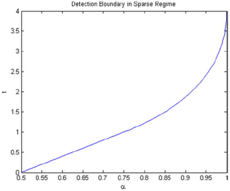
Detection boundary $t={\rho }_{\mathrm{binary}}^{\ast }(\alpha )$ in the sparse regime when θ corresponds to logistic regression. The detectable region is $t>{\rho }_{\mathrm{binary}}^{\ast }(\alpha )$, and the undetectable region is $t<{\rho }_{\mathrm{binary}}^{\ast }(\alpha )$. The curve corresponds to $t={\rho }_{\mathrm{binary}}^{\ast }(\alpha )$.

This is the same as the Gaussian detection boundary (1.1) multiplied by 1/4(θ′ (0))². The reason for the appearance of the factor 1/4(θ′ (0))² is that the Fisher information for a single Bernoulli sample under binary regression model (2.1) is equal to $\sqrt{4{({\theta }^{\prime }(0))}^2}$.

For every j ∈ {1, …, p}, we have

$${\widehat{\beta }}_j^{\mathrm{MLE}}\stackrel{d}{\to }N({\beta }_j,{\sigma }_j^2),$$

where ${\sigma }_j^2=4{({\theta }^{\prime }(0))}^2$ under H₀ and ${\sigma }_j^2\approx 4{({\theta }^{\prime }(0))}^2$ under H₁. To see this, note that under H₁ we have ${\sigma }_j^2=(\frac{1}{2}+\delta )(\frac{1}{2}-\delta )\approx 4{\theta }^{\prime }(0)$ where δ > 0 is small and denotes a departure of the Bernoulli proportion from the null value of $\frac{1}{2}$, that is, under H₁, the outcomes corresponding to the signals follow $\mathrm{Bernoulli}(\frac{1}{2}+\delta )$ or $\mathrm{Bernoulli}(\frac{1}{2}-\delta )$. This implies $\sqrt{\frac{1}{4{({\theta }^{\prime }(0))}^2}}\widehat{\mathit{\beta }}$ should yield a detection boundary similar to the multivariate Gaussian model case.

For the detection boundary in the corresponding binomial proportion model (6.1) and the testing problem (6.2), we define the following function:

$${\rho }_{\mathrm{binomial}}^{\ast }(\alpha )=\{\begin{array}{ll}\frac{(\alpha -(1/2))}{4},& \mathrm{if}\frac{1}{2}<\alpha <\frac{3}{4},\\ \frac{{(1-\sqrt{1-\alpha })}^2}{4},& \mathrm{if}\alpha \ge \frac{3}{4}.\end{array}$$ (6.4)

The following theorem provides the exact lower boundary for the ANOVA(r) designs for the binary regression model as well as the corresponding binomial problem.

Theorem 6.8

Let X ∈ ANOVA(r). Suppose r ≫ log (p) and k = p^1−α with $\alpha >\frac{1}{2}$

1. Consider the binary regression model (2.1) and the testing problem (2.3). Further suppose that θ ∈ BC² (0). Let $A=\sqrt{\frac{2t\log (p)}{r}}$. If $t<{\rho }_{\mathrm{binary}}^{\ast }(\alpha )$, all tests are asymptotically powerless.

2. Consider the binomial model (6.1) and the testing problem (6.2). Let $\mathrm{\Delta }=\sqrt{\frac{2t\log (p)}{r}}$. If $t<{\rho }_{\mathrm{binomial}}^{\ast }(\alpha )$, all tests are asymptotically powerless.

Remark 6.9

As mentioned in the Introduction, the analysis turns out to be surprisingly nontrivial since it seems not possible to simply reduce the calculations to the Gaussian case by doing a Taylor expansion of L_π around β = 0. In particular, a natural approach to analyze these problems is to expand the integrand of L_π by a Taylor series around β = 0 and thereby reducing the analysis to calculations in the Gaussian situation and a subsequent analysis of the remainder term. However, in order to find the sharp detection boundary, the analysis of the remainder term turns out to be very complicated and nontrivial. Thus, our proof to Theorem 6.8 is not a simple application of results from the Gaussian linear model.

6.2.2. Upper bound

According to Theorem 6.8, all tests are asymptotically powerless if $t<{\rho }_{\mathrm{binary}}^{\ast }(\alpha )$ in the sparse regime. In this section, we introduce tests which reach the lower bound discussed in the previous section. We divide our analysis into two subsections. In Section 6.2.2.1, we study the Higher Criticism Test defined by (5.2) which is asymptotically powerful as soon as $t>{\rho }_{\mathrm{binary}}^{\ast }(\alpha )$ in the sparse regime. In Section 6.2.2.3, we discuss a more familiar Max Test or minimum p-value test which attains the sharp detection boundary only for $\alpha \ge \frac{3}{4}$.

6.2.2.1. The Higher Criticism Test

In this section, we study the version of Higher Criticism introduced in Section 6.2. Recall, we have by Theorem 5.2 that the type I error of the Higher Criticism Test, as defined by equation (5.3), converges to 0. The next theorem states the optimality of the Higher Criticism Test as soon as the signal strength exceeds the detection boundary.

Theorem 6.10

Let X ∈ ANOVA(r). Suppose r ≫ log (p) and k = p^1−α with $\alpha >\frac{1}{2}$.

1. Consider the binary regression model (2.1) and the testing problem (2.3). Further suppose that θ ∈ BC²(0). Let $A=\sqrt{\frac{2t\log (p)}{r}}$. If $t>{\rho }_{\mathrm{binary}}^{\ast }(\alpha )$, then the Higher Criticism Test is asymptotically powerful.

2. Consider the binomial model (6.1) and the testing problem (6.2). Let $\mathrm{\Delta }=\sqrt{\frac{2t\log (p)}{r}}$. If $t>{\rho }_{\mathrm{binomial}}^{\ast }(\alpha )$, then the Higher Criticism Test is asymptotically powerful.

6.2.2.2. Comparison with the original Higher Criticism Test

We begin by providing a slight simplification of T_HC in ANOVA(r) designs. Let S be a generic Bin(r, $\frac{1}{2}$) random variable and B, B̄, respectively, denote the distribution function and the survival function of $\frac{|S-(r/2)|}{\sqrt{r/4}}$. Hence,

$$\mathrm{B}(t)=\mathbb{P}\left(\frac{|S-(r/2)|}{\sqrt{r/4}}\le t\right),\overline{\mathrm{B}}(t)=1-\mathrm{B}(t).$$

In the case of ANOVA(r) designs, $W_p(t)=\sqrt{p}\frac{{\overline{\mathrm{F}}}_p(t)-\overline{\mathrm{B}}(t)}{\sqrt{\overline{\mathrm{B}}}(t)(1-\overline{\mathrm{B}}(t))}$. The original Higher Criticism Test as defined by Donoho and Jin (2004) can also be calculated as a maximum over some appropriate function of p-values. By that token, ideally we would like to define the Higher Criticism Test statistic as

$${\mathrm{T}}_{\mathrm{HC}}^{\mathrm{Ideal}}=\underset{0<t<r/2}{\sup }{W}_p(t).$$

However, due to difficulties in calculating the null distribution for deciding a cut-off for the rejection region, we instead work with a discretized version of it. We detail this below in the context of ANOVA(r) designs. Define the jth p-value as $q_j=\mathbb{P}(|\mathrm{Bin}(r,\frac{1}{2})-\frac{r}{2}|>|Z_j-\frac{r}{2}|)$ for 1, …, p and let q₍₁₎, …, q_(p) be the ordered p-values based on exact binomial distribution probabilities. Define

$$T_{\mathrm{HC}}^{\prime }=\underset{1\le j\le p}{\max }\sqrt{p}\frac{(j/p)-(q_i)}{\sqrt{q_{(j)}(1-q_{(j)})}}.$$

It is difficult to analyze the distribution of ${\mathrm{T}}_{\mathrm{HC}}^{\prime }$ under the null to decide a valid cut-off for testing. The following proposition yields a relationship between T_HC, ${\mathrm{T}}_{\mathrm{HC}}^{\mathrm{Ideal}}$ and ${\mathrm{T}}_{\mathrm{HC}}^{\prime }$.

Proposition 6.11

Let ${|Z-\frac{r}{2}|}_{(j)}$ denote the jth order statistics based on $|Z_i-\frac{r}{2}|$, i = 1, …, p. For t such that ${|Z-\frac{r}{2}|}_{(p-j)}\le t<{|Z-\frac{r}{2}|}_{(p-j+1)}$, we have

$$\sqrt{p}\frac{{\overline{\mathrm{F}}}_p(t)-\overline{\mathrm{B}}(t)}{\sqrt{\overline{\mathrm{B}}(t)(1-\overline{\mathrm{B}}(t))}}\le \sqrt{p}\frac{(j/p)-q_{(j)}}{\sqrt{q_{(j)}(1-q_{(j)})}}.$$

Hence, from Proposition 6.11, we observe that we have the following inequality:

$${\mathrm{T}}_{\mathrm{HC}}^{\prime }\ge {\mathrm{T}}_{\mathrm{HC}}^{\mathrm{Ideal}}\ge {\mathrm{T}}_{\mathrm{HC}}.$$ (6.5)

This unlike the results in Donoho and Jin (2004) and Cai, Jeng and Jin (2011), where the leftmost inequality is a equality. Therefore, it is worth further comparing the above discussion to the Higher Criticism Test introduced by Donoho and Jin (2004), Hall and Jin (2010) in the Gaussian framework. In the case of orthogonal Gaussian linear models, T_HC, ${\mathrm{T}}_{\mathrm{HC}}^{\prime }$ and ${\mathrm{T}}_{\mathrm{HC}}^{\mathrm{Ideal}}$ are defined by standard normal survival functions and p-values, respectively, and one uses Z_j instead of $\frac{Z_j-(r/2)}{\sqrt{r/4}}$ in the definition of T_HC. This yields that in the Gaussian framework the leftmost inequality of (6.5) is an equality. Moreover, under the framework, standard empirical process results for continuous distribution functions yield asymptotics for ${\mathrm{T}}_{\mathrm{HC}}^{\mathrm{Ideal}}$ under the null. Therefore, in the Gaussian case the uncountable supremum in the definition of ${\mathrm{T}}_{\mathrm{HC}}^{\mathrm{Ideal}}$ is attained and the statistic is algebraically equal to a maximum over finitely many functions of p-values, namely, ${\mathrm{T}}_{\mathrm{HC}}^{\prime }$. However, due to the possibility of strict inequality in Proposition 6.11 for the binomial distribution, we cannot reduce our computation to p-values as in the Gaussian case. Although it is true that marginally each q_j is stochastically smaller than a U(0, 1) random variable, we are unable to find a suitable upper bound for the rate of ${\mathrm{T}}_{\mathrm{HC}}^{\prime }$ since it also depends on the joint distribution of q₍₁₎, …, q_(p). It might be possible to estimate the gaps between ${\mathrm{T}}_{\mathrm{HC}}^{\prime }$, ${\mathrm{T}}_{\mathrm{HC}}^{\mathrm{Ideal}}$ and T_HC, but since this is not essential for our purpose, we do not attempt this.

6.2.2.3. Rate optimal upper bound: Max Test

A popular multiple comparison procedure is the minimum p-value test. In the context of Gaussian linear regression, Donoho and Jin (2004) and Arias-Castro, Candès and Plan (2011) showed that the minimum p-value test reaches the sharp detection boundary if and only if $\alpha \ge \frac{3}{4}$. In this section, we introduce and study the minimum p-value test in binary regression models.

As before, define the jth p-value as

$$q_j=\mathbb{P}\left(\left|\mathrm{Bin}\left(r,\frac{1}{2}\right)-\frac{r}{2}\right|>\left|Z_j-\frac{r}{2}\right|\right)$$

for j = 1, …, p and let q₍₁₎, …, q_(p) be the ordered p-values. We will study the test based on the minimum p-value q₍₁₎. Note that it is equivalent to study the test based on the statistic

$$\underset{1\le j\le p}{\max }{W}_j,W_j=\frac{|Z_j-(r/2)|}{\sqrt{r/4}}.$$

From now on, we will call this the Max Test. In the following theorem, we show that similar to Gaussian linear models, for binary regression, the Max Test attains the sharp detection boundary if and only if $\alpha \ge \frac{3}{4}$. However, if one is interested in rate optimal testing, that is, only the rate or order of the detection boundary rather than the exact constants, the Max Test continues to perform well in the entire sparse regime.

Theorem 6.12

Let X ∈ ANOVA(r). Suppose r ≫ (log r)² log(p) and k = p^1−α with $\alpha >\frac{1}{2}$.

1. Suppose θ ∈ BC² (0) and let $A=\sqrt{\frac{2t\log (p)}{r}}$. Set ${\rho }_{\mathrm{Max},\mathrm{binary}}^{\ast }(\alpha )=\frac{{(1-\sqrt{1-\alpha })}^2}{4{({\theta }^{\prime }(0))}^2}.$

   Then in the model (2.1) and problem (2.3) one has the following:

   1. If $t>{\rho }_{\mathrm{Max},\mathrm{binary}}^{\ast }(\alpha )$, then the Max Test is asymptotically powerful.

   2. If $t<{\rho }_{\mathrm{Max},\mathrm{binary}}^{\ast }(\alpha )$, then the Max Test is asymptotically powerless.

2. Let $\mathrm{\Delta }=\sqrt{\frac{2t\log (p)}{r}}$. Set ${\rho }_{\mathrm{Max},\mathrm{binomial}}^{\ast }(\alpha )=\frac{{(1-\sqrt{1-\alpha })}^2}{4}$. Then in the model (6.1) and problem (6.2) one has the following:

   1. If $t>{\rho }_{\mathrm{Max},\mathrm{binomial}}^{\ast }(\alpha )$, then the Max Test is asymptotically powerful.

   2. If $t<{\rho }_{\mathrm{Max},\mathrm{bionmial}}^{\ast }(\alpha )$, then the Max Test is asymptotically powerless.

Theorem 6.12 implies that the detection boundary for the Max Test matches the detection boundary of the Higher Criticism Test only for $\alpha \ge \frac{3}{4}$. For $\alpha <\frac{3}{4}$, the detection boundary of the Max Test lies strictly above that of the Higher Criticism Test. Hence, the Max Test fails to attain the sharp detection boundary in the moderate sparsity regime, $\alpha <\frac{3}{4}$. Thus, if one is certain of high sparsity it can be reasonable to use the Max Test whereas the Higher Criticism Test performs well throughout the sparse regime. It is worth noting that the requirement r ≫ (log(r))² log(p) is a technical constraint and can be relaxed. In most situations, it does not differ much from the actual necessary condition r ≫ log(p), and hence we use r ≫ (log(r))² log(p) for proving Theorem 6.12.

7. Detection boundary and asymptotic analysis for Weakly Correlated Designs

In this section, we study the role of the parameter vector (n*,n_*, r*, r_*,Q_n,p, γ_n,p) in deciding the detection boundary for Weakly Correlated Designs defined in Definition 4.1. For the sake of brevity, we will often drop the subscripts n, p from Q and γ when there is no confusion. Recall Ω* from Section 4.

If we just concentrate on the observations corresponding to the rows with index in Ω*, we have an orthogonal design matrix similar to ANOVA(r) designs. Our proofs of lower bounds in both dense and sparse regimes and also the test statistics proposed for the attaining the sharp upper bound is motivated by this fact. Similar to ANOVA(r) designs, we divide our analysis into the dense and sparse regimes. Also, owing to the possible nonorthogonality of X for Weakly Correlated Designs, we cannot directly reduce this problem to testing homogeneity of binomial proportions as in (6.2). So, henceforth, we will be analyzing model (2.1) and corresponding testing problem (2.3). However, as we shall see, under certain combinations of (n*,n_*, r*, r_*,Q, γ), one can essentially treat the problem as an orthogonal design like in ANOVA(r) designs. This is explained in the following two sections.

7.1. Dense regime $(\alpha \le \frac{1}{2})$

We recall the definition of the GLRT from equation (5.1). The following theorem provides the lower and upper bound for the dense regime.

Theorem 7.1

Let X be a Weakly Correlated Design as in Definition 4.1. Suppose Let k = p^1−α with $\alpha \le \frac{1}{2}$ and r_* > 1. Assume θ ∈ BC²(0) and set γ = p^(1/2)−α. Then we have the following:

1. If $A\ll \sqrt{\frac{p^{1/2}}{k{r}^{\ast }}}$, then all tests are asymptotically powerless.

2. If $A\gg \sqrt{\frac{p^{1/2}}{k{r}_{\ast }}}$, then the GLRT is asymptotically powerful.

We note that the form of the detection boundary is exactly same as that in Theorem 6.5 for ANOVA(r) designs with r* and r_* playing the role of r. This implies that when n_*Q² is not too large ( $\frac{n_{\ast }{Q}^2}{r^{\ast }}\ll \gamma =p^{\left(1/2\right)-\alpha }$); we can still recover the same results as in ANOVA(r) designs because the columns of the design matrix are weakly correlated.

7.2. Sparse regime $(\alpha >\frac{1}{2})$

Unlike the dense regime, the sparse regime depends more heavily on the values of r* and r_*. The next theorem quantifies this result; it shows that in the sparse regime if r* ≪ log(p), then all tests are asymptotically powerless. This result is analogous to Theorem 6.6 for ANOVA(r) designs. Indeed this can be argued from Theorems 3.1 and 3.2. However, for the sake of completeness, we provide it here.

Theorem 7.2

Let X be a Weakly Correlated Design as in Definition 4.1. Let k = p^1−α with $\alpha >\frac{1}{2}$ and let |∪_i∉Ω* S_i| ≪ p. If r* ≪ log(p), then all tests are asymptotically powerless.

Remark 7.3

The condition |∪_i∉Ω* S_i| ≪ p, restricts the location of nonzero elements in the support of rows of X when the row has more than one nonzero element. This restriction imposes a structure on the deviation of X from orthogonality. As the proof of Theorem 7.2 will suggest, this condition ensures that the assumptions of Theorem 3.1 hold, and hence renders all tests asymptotically powerless irrespective of signal strength.

The following theorem provides the value of γ that is defined in condition (C3) in Definition 4.1, to ensure the results parallel to Theorem 6.8. Not surprisingly, the test attaining the sharp lower bound turns to be the version of the Higher Criticism Test introduced in Section 6. Similar to the ANOVA(r) design, it is also possible to introduce and study the Max Test which attains the sharp detection boundary only for $\alpha \ge \frac{3}{4}$. However, we omit this since it can be easily derived from the existing arguments.

Theorem 7.4

Let X be a Weakly Correlated Design as in Definition 4.1 and k = p^1−α with $\alpha >\frac{1}{2}$. Suppose r_* ≫ log(p), γ = log(p), where γ is defined in Definition 4.1. Further suppose that θ ∈ BC²(0).

1. Let $A=\sqrt{\frac{2t\log \left(p\right)}{r^{\ast }}}$. If $t<{\rho }_{\mathrm{binary}}^{\ast }(\alpha )$, then all tests are asymptotically powerless.

2. Let $A=\sqrt{\frac{2t\log \left(p\right)}{r_{\ast }}}$. If $t>{\rho }_{\mathrm{binary}}^{\ast }\left(\alpha \right)$, then the Higher Criticism Test is asymptotically powerful.

Remark 7.5

The assumptions on the design matrix in Theorem 7.4 is weaker than the assumptions in Theorem 7.2. In particular, one is allowed to go beyond |∪_i∉Ω* S_i| ≪ p in Theorem 7.2 as long as the condition (C3) is satisfied with γ = log(p). This is expected since the conditions under which all tests are asymptotically powerless irrespective of sample size are often more stringent.

Remark 7.6

Theorem 7.4 states that the Higher Criticism Test attains the sharp detection boundary in the sparse regime. Note that the difference in the denominators of A in the statement of upper and lower bound in Theorem 7.4 is unavoidable and the difference vanishes asymptotically if r*/r_* → 1. This is expected since the detection boundary depends on the column norms of the design matrix.

8. Simulation studies

We complement our study with some numerical simulations which illustrate the empirical performance of the test statistics described in earlier sections for finite sample sizes. Since detection complexity of the general weakly correlated binary design matrices depend on the behavior of ANOVA(r) type designs, we only provide simulations for strong one-way ANOVA type design. Let X be a balanced design matrix with p = 10,000 covariates and r replicates per covariate. For different values of sparsity index α ∈ (0, 1) and r, we study the performance of Higher Criticism Test, GLRT and Max Test, respectively, for different values of t, where t which corresponds to $A=\sqrt{\frac{2({\rho }_{\mathrm{logistic}}^{\ast }\left(\alpha \right)+t)\log \left(p\right)}{r}}$.

Following Arias-Castro, Candès and Plan (2011), the performance of each of the three methods is computed in terms of the empirical risk defined as the sum of probabilities of type I and II errors achievable across all thresholds. The errors are averaged over 300 trials. Even though the theoretical calculation of null distribution of the Higher Criticism Test statistic computed from p-values remains a challenge, we found that using the p-value based statistic ${\max }_{1\le j\le p/2}\sqrt{p}\frac{(j/p)-q_{(j)}}{\sqrt{q_{(j)}(1-q_{(j)})}}$ yielded expected results similar to our version of discretized Higher Criticism.

To be precise, the performance of the test based on ${\max }_{1\le j\le p/2}\sqrt{p}\frac{(j/p)-q_{(j)}}{\sqrt{q_{(j)}(1-q_{(j)})}}$ was similar to the performance of the test based on T_HC defined in Section 5.2. Note that this statistic is different from $T_{\mathrm{HC}}^{\prime }$ in that the maximum is taken over the first $\frac{p}{2}$ elements instead of all p of them. The main reason for this is the fact that, as noted by Donoho and Jin (2004), the information about the signal in the sample lies away from the extreme p-values. The GLRT is based on T_GLRT as defined in Section 5.1 and the Max Test is based on the test statistic defined in Section 6.2.2.3.

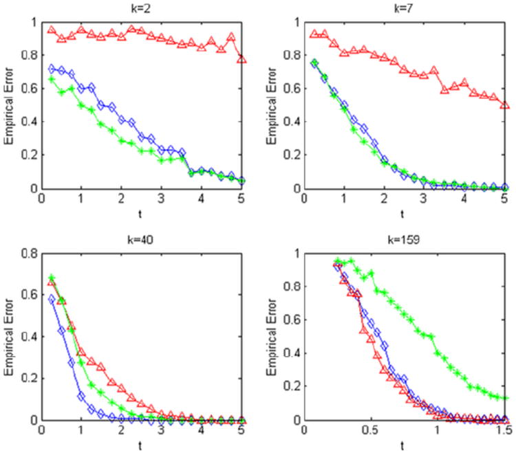
The results are reported in Figures 4 and 5. For $r=\sqrt{\log \left(p\right)}\ll \log \left(p\right)$ and k = 2, 7 which corresponds to $k\ll \sqrt{p}$, that is, the sparse regime, we can see that all tests are asymptotically powerless in Figure 4 which is expected from the theoretical results. However, even when $r=\lceil \sqrt{\log \left(p\right)}\rceil \ll \log \left(p\right)$, for the dense regime, and k = 159 and 631, we see from Figure 4 that the GLRT is asymptotically powerful whereas the other two tests are asymptotically powerless. Once r is much larger than log(p) in Figure 5, our observations are similar to Arias-Castro, Candès and Plan (2011). Here, we employ simulations for k = 2, 7, 40 which correspond to the sparse regime and for k = 159 which corresponds to the dense regime. We note that the performance of GLRT improves very quickly as the sparsity decreases and begins dominating the Max Test. The performance of the Max Test follows the opposite pattern with errors of testing increasing as k increases. The Higher Criticism Test, however, continues to have good performance across the different sparsity levels once r ≫ log(p).

Fig. 4.

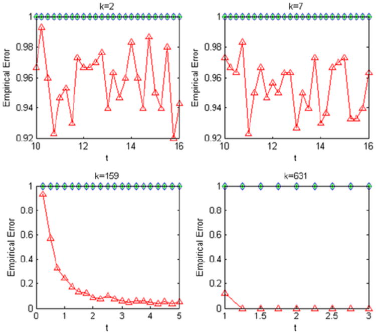
Simulation results are for p = 10,000 and $r=\lceil \sqrt{\log (p)}\rceil =4$. Sparsity level k is indicated below each plot. In each plot, the empirical risk of each method [GLRT (triangles); Higher Criticism (diamonds); Max Test (stars)] is plotted against t which corresponds to $A=\sqrt{\frac{\max \{2({\rho }_{\mathrm{logistic}}^{\ast }(\alpha )+t),0\}\log (p)}{r}}$.

Fig. 5.

Simulation results are for p = 10,000 and $r=\lceil {\left(\log (p)\right)}^5\rceil =66,280$. Sparsity level k is indicated below each plot. In each plot, the empirical risk of each method [GLRT (triangles); Higher Criticism (diamonds); Max Test (stars)] is plotted against t which corresponds to $A=\sqrt{\frac{2({\rho }_{\mathrm{logistic}}^{\ast }(\alpha )+t)\log \left(p\right)}{r}}$.

9. Discussions

In this paper, we study testing of the global null hypothesis against sparse alternatives in the context of general binary regression. We show that, unlike Gaussian regression, the problem depends not only on signal sparsity and strength, but also heavily on a design matrix sparsity index. We provide conditions on the design matrix which render all tests asymptotically powerless irrespective of signal strength. In the special case of design matrices with binary entries and certain sparsity structures, we derive the lower and upper bounds for the testing problem in both dense (rate optimal) and sparse regimes (sharp including constants). In this context, we also develop a version of the Higher Criticism Test statistic applicable for binary data which attains the sharp detection boundary in the sparse regime.

In this paper, we constructed tests by combining tests based on Z-statistics from the orthogonal part and the nonorthogonal part of the X. In particular, we combine procedures based on Z_j and $Z_j^{\mathbf{G}}$ separately. This helps us achieve optimal rates for upper bounds on testing errors under the same conditions required for lower bounds in these problems. Indeed, one can consider constructing GLRT and Higher Criticism Test using Z-statistics constructed based on whole X, that is, based on $Z_j^{\mathbf{X}}=X_j^{T}y$, j = 1,…, p directly. We could obtain similar results based on the combined Z-statistics under stronger structural information on G than what we require here.

In particular, the conditions regarding the relative size of G with respect to the orthogonal part of the design matrix, can be substantially relaxed if more structural assumptions on G are made. For example, for sequencing data, as observed in the Dallas Heart study data, for people having more than one mutation, the locations of the mutations are in fact usually clustered, due to linkage disequilibrium. For such structures, strong results can be obtained. We omit those results here due to space limitation. Future research is also needed to study the detection boundary for binary regression for more general design matrices.

The study of detection boundaries associated with binary regression models for a general design matrix is much more delicate. We allow in this paper for a more general sparse design when the nonorthogonal columns of the design matrix are sufficiently sparse and the number of subjects with multiple nonzero entries in the design matrix are not too large. Future research is needed to extend the results to a general design matrix allowing a stronger correlation among the covariates X_j ’s.

Supplementary Material

AOS1279

Supplement to “Hypothesis testing for high-dimensional sparse binary regression” (DOI: 10.1214/14-AOS1279SUPP;.pdf). The supplementary material contain the proofs of all theorems, propositions and supporting lemmas.

References

- Arias-Castro E, Candès EJ, Plan Y. Global testing under sparse alternatives: ANOVA, multiple comparisons and the higher criticism. Ann Statist. 2011;39:2533–2556. MR2906877. [Google Scholar]
- Baraud Y. Non-asymptotic minimax rates of testing in signal detection. Bernoulli. 2002;8:577–606. MR1935648. [Google Scholar]
- Cai TT, Jeng XJ, Jin J. Optimal detection of heterogeneous and heteroscedastic mixtures. J R Stat Soc Ser B Stat Methodol. 2011;73:629–662. MR2867452. [Google Scholar]
- 1000 Genomes Project Consortium and others. An integrated map of genetic variation from 1,092 human genomes. Nature. 2012;491:56–65. doi: 10.1038/nature11632. [DOI] [PMC free article] [PubMed] [Google Scholar]
- Donoho D, Jin J. Higher criticism for detecting sparse heterogeneous mixtures. Ann Statist. 2004;32:962–994. MR2065195. [Google Scholar]
- Fu W, O’Connor TD, Jun G, Kang HM, Abecasis G, Leal SM, Gabriel S, Rieder MJ, Altshuler D, Shendure J, et al. Analysis of 6,515 exomes reveals the recent origin of most human protein-coding variants. Nature. 2013;493:216–220. doi: 10.1038/nature11690. [DOI] [PMC free article] [PubMed] [Google Scholar]
- Hall P, Jin J. Innovated higher criticism for detecting sparse signals in correlated noise. Ann Statist. 2010;38:1686–1732. MR2662357. [Google Scholar]
- Ingster YuI, Suslina IA. Lecture Notes in Statistics. Vol. 169. Springer; New York: 2003. Nonparametric Goodness-of-Fit Testing Under Gaussian Models. MR1991446. [Google Scholar]
- Ingster YI, Tsybakov AB, Verzelen N. Detection boundary in sparse regression. Electron J Stat. 2010;4:1476–1526. MR2747131. [Google Scholar]
- Komlós J, Major P, Tusnády G. An approximation of partial sums of independent RV’s and the sample DF. I. Z Wahrsch Verw Gebiete. 1975;32:111–131. MR0375412. [Google Scholar]
- Lee S, Abecasis G, Boehnke M, Lin X. Analysis of rare variants in sequencing-based association studies. The American Journal of Human Genetics. 2014;95:5–23. [Google Scholar]
- Mukherjee R, Pillai NS, Lin X. Supplement to “Hypothesis testing for high-dimensional sparse binary regression”. 2014 doi: 10.1214/14-AOS1279SUPP. [DOI] [PMC free article] [PubMed] [Google Scholar]
- Nelson MR, Wegmann D, Ehm MG, Kessner D, Jean PS, Verzilli C, Shen J, Tang Z, Bacanu SA, Fraser D, et al. An abundance of rare functional variants in 202 drug target genes sequenced in 14,002 people. Science. 2012;337:100–104. doi: 10.1126/science.1217876. [DOI] [PMC free article] [PubMed] [Google Scholar]
- Plan Y, Vershynin R. One-bit compressed sensing by linear programming. Comm Pure Appl Math. 2013a;66:1275–1297. MR3069959. [Google Scholar]
- Plan Y, Vershynin R. Robust 1-bit compressed sensing and sparse logistic regression: A convex programming approach. IEEE Trans Inform Theory. 2013b;59:482–494. MR3008160. [Google Scholar]
- Tang H, Jin X, Li Y, Jiang H, Tang X, Yang X, Cheng H, Qiu Y, Chen G, Mei J, et al. A large-scale screen for coding variants predisposing to psoriasis. Nature Genetics. 2014;46:40–50. doi: 10.1038/ng.2827. [DOI] [PubMed] [Google Scholar]
- Victor RG, Haley RW, Willett DL, Peshock RM, Vaeth PC, Leonard D, Basit M, Cooper RS, Iannacchione VG, Visscher WA, et al. The Dallas Heart Study: A population-based probability sample for the multidisciplinary study of ethnic differences in cardiovascular health. The American Journal of Cardiology. 2004;93:1473–1480. doi: 10.1016/j.amjcard.2004.02.058. [DOI] [PubMed] [Google Scholar]
Associated Data
This section collects any data citations, data availability statements, or supplementary materials included in this article.
Supplementary Materials