From within-host interactions to epidemiological competition: a general model for multiple infections

Abstract

Many hosts are infected by several parasite genotypes at a time. In these co-infected hosts, parasites can interact in various ways thus creating diverse within-host dynamics, making it difficult to predict the expression and the evolution of virulence. Moreover, multiple infections generate a combinatorial diversity of cotransmission routes at the host population level, which complicates the epidemiology and may lead to non-trivial outcomes. We introduce a new model for multiple infections, which allows any number of parasite genotypes to infect hosts and potentially coexist in the population. In our model, parasites affect one another's within-host growth through density-dependent interactions and by means of public goods and spite. These within-host interactions determine virulence, recovery and transmission rates, which are then integrated in a transmission network. We use analytical solutions and numerical simulations to investigate epidemiological feedbacks in host populations infected by several parasite genotypes. Finally, we discuss general perspectives on multiple infections.

1. Introduction

There is increasing evidence that multiple parasite strains or species infecting the same host is a common context of parasitism in the wild [1–4]. These co-infections occur for several host–parasite interactions that range from bacteria infected by bacteriophage viruses to animals or plants infected by viruses, bacteria or worms [5,6]. In addition to being a major concern in public health, human and veterinary medicine and phytopathology, co-infections are also a challenging subject for ecology and evolution. In a co-infected host, the different strains or species of parasites (hereafter referred to as ‘genotypes’) can interact in various ways [7–9]. For instance, some symbiont bacteria produce siderophores that harvest iron for the whole microbiota [10], whereas others produce bacteriocins that break down the bacterial cell envelope [11]. Such processes generate diverse within-host dynamics that make it difficult to predict the evolution or even sometimes the expression of the ‘overall virulence’ [12,13], i.e. the additional host mortality rate in the co-infected host. Moreover, considering multiple infections at the host population level generates a combinatorial diversity of (co)transmission routes, which complicates the epidemiology. This can lead to non-trivial outcomes of epidemics involving multiple genotypes.

The unpredictable outcome of the within-host interactions between parasites and the combinatorial complexity of the cotransmissions are probably the two main reasons why the vast majority of epidemiological models still lean on classical SIR (susceptible, infected, removed) models [14,15] which consider only one parasite genotype infecting a population of hosts. Models allowing for several genotypes are often restricted to two strains [16,17] or arbitrarily choose between a superinfection pattern [16,18] and a co-infection pattern [12,17,19]. In superinfections, parasite genotypes cannot coexist within the host and one always outcompetes the others. In co-infections, within-host coexistence is made possible but these models usually rely on strong assumptions such as no within-host interactions [19], fixed relatedness [20] or epidemiological equivalence between genotypes [21].

Physiological and epidemiological observations render the state of the art of modelling multiple infections unsatisfying. For instance, it is obvious that dividing the reality between co-infections (always coexistence) and superinfection (never coexistence) is oversimplifying. In several pathogens, for instance, coexistence can be only transitory and one of the genotypes can eventually exclude the others, as shown in the case of rodent malaria [22]. Furthermore, arbitrarily limiting the number of genotypes per host to two is oversimplifying, as shown, for example, in the case of human malaria [3]. A final unsatisfying model limitation is that parasites only interact through one type of process. Yet, it is known that bacteria, for instance, can simultaneously compete for host resources, produce public goods (PGs) and spite [23].

Here, we develop a new model for multiple infections, which captures many kinds of within-host outcomes, while allowing for an arbitrary number of parasite genotypes. We based our approach on nesting the within-host parasite growth into the between-host epidemiology. Nested models have already been investigated in epidemiology to study multiple infections, either by modelling exploitation competition through host resource use [24], or immune cell infection dynamics by viruses [25,26]. However, existing nested models (reviewed in [27]) often ignore several within-host processes, such as within-host parasite interactions, and force the outcome of infection (superinfection or co-infection). By explicitly allowing parasite genotypes to affect one another's within-host growth in more than one way, through the production of PGs, spite, competition for host resources or interactions with the host immune system, we do not need to make assumptions such as superinfection or co-infection. Such states appear as outcomes of the within-host interactions. We then use these within-host outcomes to define infection, recovery and death rates, allowing for partial cotransmission (i.e. we do not impose constraints on which genotype combination an infected host transmits) and numerically simulate epidemics.

We show that relaxing assumptions commonly made leads to rich and complex behaviour of the epidemics, because of epidemiological feedbacks. Such feedbacks could not be captured by previous models based solely on within-host dynamics [20] because they failed to integrate the between-host level. Here, we also propose a methodology to capture these feedbacks when estimating the basic reproduction number, that is the number of secondary infections caused by an infected host in a fully susceptible host population during its entire period of infectiousness [28].

2. Within-host dynamics

The first challenging step is to model the within-host growth of an arbitrary number of unrelated genotypes by taking into account several processes. Indeed, current models typically, though not always, only involve a single process and/or at most two genotypes. To this end, we assume that the parasite load of each genotype follows a quadratic ordinary differential equation (ODE) inspired by the classical framework of population dynamics [29]. Besides constant basic growth and density-dependent feedback, we allow the instantaneous parasite growth to be affected by molecules they produce: PGs and spite. We present the equations and main assumptions before solving the system at steady state.

We consider an arbitrary number n ∈ ℕ^★ of parasite genotypes which are not necessarily related nor from the same species (all the notations used thereafter are summarized in the electronic supplementary material, appendix A). Each genotype is defined by a set of within-host traits, which are assumed to be constant (no plasticity). We denote the set of parasite genotypes (where : = means ‘equals by definition’). We wish to model the variation with continuous time t of the parasite load vector in a host co-infected by all n genotypes.

(a). Public production dynamics

Parasites such as symbiotic bacteria can produce and secrete molecules in the (within-host) environment [13]. Because any genotype can be affected by molecules produced by another genotype, we refer to these as public productions (PPs). PP can have positive effects on the growth of the receiver. This is the case for siderophores [30] and more generally, what we refer to as PGs [9]. PPs can also be detrimental to the receiver as in the case of bacteriocins [11] and we refer to this as spite [31]. 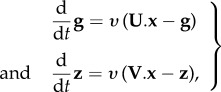We assume each genotype can produce at most one type of PG and one type of spite, implying there are 2n concentrations of molecules that also vary with time, respectively, for PG and for spite. We assume that PPs are produced by the parasites at a constant rate, independently of the current PPs, and are cleared in a non-specific but concentration-dependent way at a standard rate υ. Overall, the dynamics of the PP concentrations follow

2.1

where and are the diagonal matrices of PP production rates standardized by υ.

(b). Parasite load dynamics

PGs increase parasite growth rate, while spite molecules decrease it. We assume that these effects linearly depend on the molecule concentrations, which are spatially homogeneous. One type of PP can have different effects depending on the genotype of the receiver. We can define the matrix of PG effects on growth rate , where γ_k,j > 0 is the effect of the PG type produced by genotype j on the growth of genotype k. Likewise, is the matrix of spite effects on growth rate, where σ_k,j > 0 is the effect (in absolute value) of the spite type produced by genotype j on the growth rate of genotype k if k ≠ j. We assume a genotype is not affected by its own spite type (that is σ_k,k = 0).

In addition to these within-host secreted PPs, we group all the other genotype-to-genotype interactions into called the matrix of density-dependent effects, where η_k,j ∈ ℝ is the density-dependent effect of genotype j on the growth rate of genotype k. These density-dependent effects could reflect competition for host resources, indirect interactions through the elicitation of the host immune system or any other within-host process through which parasites could interact. Note that Γ, Σ and H are not necessarily symmetrical.

Finally, with ϱ: = (ϱ_k)_k∈𝒢 being the basic growth rate vector, the parasite load vector x satisfies the following ordinary nonlinear differential equation:

2.2

where ⊙ denotes the Hadamard (element-wise) matrix product. As the basic growth rate takes place in the only linear term of equation (2.2), it actually captures not only the rate at which a parasite genotype would grow at first if isolated but also the cost of PG and spite production.

The within-host dynamics are summarized in figure 1. Note that the total number of parameters for this part of the model is 3n² + 2n + 1.

Figure 1.

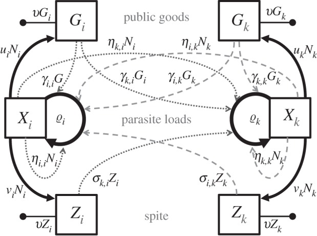
Within-host flow diagram for two different genotypes i and k. Plain arrows represent PP flows, while dotted-ended arrows represent PP clearance flows. Dotted arrows and dashed arrows are per capita growth rate modulation effects generated by genotype i parasites and by genotype k parasites, respectively. PGs (G_i and G_k) increase the growth of all genotypes (X_i and X_k), while spite (Z_i and Z_k) only harms the other genotype.

(c). Steady state

These within-host dynamics are complex and, as explained in the next section, we will often need to summarize them using their steady state. We denote by .^ a steady-state value of a variable. The steady-state vectors and cancel out in equations (2.1), thus leading to two equalities

2.3

Therefore, a within-host equilibrium is fully determined by the parasite load vector

If we assume, for the moment, that the values of are non-zero, setting equation (2.2) to 0 and using equation (2.3), it is straightforward that the only steady-state parasite load vectors are the ones that satisfy

2.4

where M is the constant matrix sum

2.5

thereafter called stationary interaction matrix.

Usually, and for random sets of parameter values, M is not singular. This implies that is unique and analytically found as

2.6

In the special case where the determinant of M is 0, equation (2.4) has an infinite number of solutions and there is no other option than to numerically integrate the within-host system (equations (2.1) and (2.2)).

Let us now relax our assumption of non-zero values of This makes sense when a particular genotype did not take part in the host inoculation, implying that its parasite load is always equal to 0. We then consider a partial combination of genotypes, that is to say any proper subset i of . The rows of equation (2.2) associated with the genotypes that do not belong to i are tautological at steady state and therefore are removed. The new set of equations we obtain satisfies the assumption of non-zero steady-state values. The solution of equation (2.6), restricted to the rows that belong to i, is the unique steady-state parasite load associated to the partial combination of genotypes i which we denote (see proof in the electronic supplementary material, appendix B.1).

3. Linking the within- and between-host levels

To eventually make inferences at the between-host level, we need to somehow simplify the within-host dynamics. In this part, we introduce the class concept, which gives an epidemiological meaning to partial genotype combinations. We also nest within-host outcomes into the between-host dynamics based on the assumption that the within-host steady state is quickly reached. Put differently, we impose a time-scale separation between the two levels. This assumption is commonly used in nested models [27]. Note that we identify a case where it cannot be satisfied (when there is unlimited within-host growth) and present a way of handling this situation via what we call ultrainfection.

(a). Host and inoculum classes

We define a class as any combination of genotypes. As there are genotypes, there are classes, which is the power set of . Mathematically, a class is any element i of . We call susceptible a host infected by no genotype (the class of which is the empty set ∅). We call singly infected host a host infected by only one genotype and co-infected host a host infected by at least two different genotypes. We call rank of a given class i the number of genotypes that belong to i, that is For computational purposes, it is useful to order these classes which is why we introduce a binary labelling operator in the electronic supplementary material, appendix C.1.

Once a host is infected by a genotype combination, it may transmit any subset of its co-infecting genotypes. We call inoculum a combination of genotypes transmitted by an infected host. The set of all possible inocula is also We assume that hosts infected by the same genotype combination are identical in every point. We also make no difference between inocula containing the same genotype combination, even if they originate from hosts infected by different genotype combinations.

(b). Ultrainfection and constraints on susceptible and single-infection classes

The susceptible state is unstable if parasites grow in a singly infected host, i.e. if ϱ_k > 0, which we will assume from now on (the proof is shown in the electronic supplementary material, appendix C.3, and involves the expression of the within-host jacobian matrix calculated in electronic supplementary material, appendix C.2). As a consequence, no infection can end by the extinction of all genotypes: either the within-host dynamics reach a steady state or at least one parasite load goes to infinity. In order to avoid the latter case (because it is not compatible with the time-scale separation assumption), we invoke two modelling assumptions from the between-host dynamics, namely

• (i) the infected host death rate is proportional to the total parasite load; and

• (ii) the size of the host population is constant.

Following these assumptions, if a host is infected by an inoculum that causes an infinite within-host parasite growth, its death rate is infinite (i); it thus dies instantaneously upon infection and is replaced by a susceptible host (ii). To picture this, one can think of a singly infected host that would become infected by another parasite genotype which facilitates the growth of the first genotype, and vice versa, such that both parasite loads increase endlessly. If we assume that this process is much faster than the transmission process and that very high parasite loads eventually lead to host death, the host will die before infecting another host and is thus epidemiologically irrelevant. We call this case ultrainfection as it cannot be considered within the superinfection–co-infection framework.

The drawback of allowing ultrainfection is that some parameter sets might result in genotypes that do not reach a steady state in any class, such that the between-host dynamics would be in fact governed by an effective number of genotypes n′ smaller than n. To avoid these ‘shadow genotypes’, one solution is to force the steady state in single infections to be both positive and stable. When a susceptible is infected by only one genotype, let us say k, the infected steady-state parasite load is then and its value is given by equation (2.6) applied for n = 1,

3.1

Given that ϱ_k > 0, the single-infection parasite load is positive and stable if and only if (for the proof of the stability, see electronic supplementary material, appendix C.4)

3.2

As the effect of PG on self and its production rate are both assumed to be positive, this implies that the self-density-dependent effect is negative (η_k,k < 0). One can interpret 1/η_k,k as the carrying capacity. Inequality (3.2) will be checked for all parameter sets used thereafter.

(c). Biological and epidemiological co-infection classes

When at least two genotypes co-infect the same host, finding the steady state reached by the system is a mathematical challenge for several reasons:

• (i) the number of possible steady states is an exponential function of the class rank,

• (ii) the stability of a steady state cannot be analytically deduced from the parameters in the general case,

• (iii) several steady states can be biologically meaningful at the same time, i.e. positive and stable (found with numerically computed eigenvalues), and

• (iv) the nonlinearity of the system causes unpredictability of the output given the initial conditions.

This leaves us with no other option than to numerically simulate higher rank infection events as follows.

First, we have to withdraw from the analysis all the host classes for which the associated (unique) steady state is not biologically meaningful. We thus say that an infected class is biological if its associated steady state is both positive and stable. Even though it is unstable and zero valued, the susceptible class is considered as a biological class too. We denote the set of biological classes by ℬ ⊂ Note that the set of inocula arising from hosts that belong to ℬ can be greater than ℬ itself. For instance, let k be a genotype absent from class i and let i ∪ {k} be a biological class. If genotype k is such that it stabilizes the within-host dynamics in a host of class i ∪ {k} (by limiting the growth of highly spite-producing genotypes for example), i may not be a biological host class even though i is a possible inoculum because it can be produced by biological class i ∪ {k} hosts.

A class may be biologically meaningful but epidemiologically meaningless if no infection event leads to it. For this reason, we define the infection operator ϕ which has two arguments, the receiver host class r and the inoculum class p. ϕ(r, p) is the output class, that is the class into which a host from class r turns if it is infected by class inoculum. In terms of system dynamics theory, ϕ(r, p) is the class associated to the potentially new steady state the within-host system reaches after the perturbation corresponding to the inoculation. We show in the electronic supplementary material, appendix C.6, that non-steady-state attractors can be avoided if the self-density-dependent effects η_k,k are negative and strong enough and if PP rates u_k and v_k are small enough. Note that ϕ(r, p) can be the empty set because ultrainfection is allowed for co-infected classes.

A biological infected class i is said to be epidemiological if it can appear during an epidemic, that is if there is at least one infection event involving two biological classes that leads to it. More formally, class i is epidemiological if there is a couple of biological classes (r, d) ∈ ℬ², r being the receiver host class and d the donor host class, such that there exists an inoculum class p of d that satisfies ϕ(r, p) = i. As an exception, the susceptible class is also epidemiological. The set of epidemiological classes is denoted by ℰ (and ℰ if the susceptible class is excluded).

If a class is not epidemiological, then there is no infection event to renew these hosts that inevitably recover or die, even if initially present. After some time, this non-epidemiological compartment has completely vanished with no other consequence than having delayed an initial input of susceptibles. For this reason, we only consider epidemiological classes in the between-host dynamics of our model.

For formal definitions of ℬ, ϕ and ℰ, see the electronic supplementary material, appendix C.5.

4. Between-host dynamics

In this part, we use the steady-state parasite loads and the previously introduced class system to define the compartments and the flow rates of a deterministic between-host dynamical system. This system is conceived as an extended SIS (susceptible, infected, susceptible) model with sequential recovery in a randomly mixed host population of constant size, which is a common framework in modelling of infectious diseases [12]. However, unlike previous models where transmission is also sequential (that is only one genotype at a time) [21], this model allows for partial cotransmission, that is the possibility for any host class to transmit any subset of genotypes it is co-infected with. A consequence of this is that suceptibles can directly turn into co-infected hosts. Assuming also that the overall transmission rate is constant, the appropriate infection rate for partial cotransmission is given hereafter.

(a). Infected hosts dynamics

Due to the time-scale separation, infected hosts from the same class have the same parasite load. Each host class is then considered as a compartment characterized by its proper time-dependent density . Note that the index-set notation is analogous to the one used in Andreasen et al. [32] for cross-immunity. These host class densities (at most 2ⁿ) define the density vector

Infection events are due to uniformly random encounters between two hosts of different classes. The donor host can infect the receiver host with any class of inoculum it may generate (any non-empty subset of its class), independently of the parasite genotypes the receiver is already infected by.

Recovery is allowed for every infected host class but only sequentially, which means that a given host can only recover from one parasite genotype at a time. Moreover, it does not provide any immunization. The between-host part of our model can therefore be seen as a generalization to multiple infections of the classical SIS model [33].

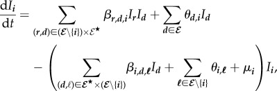
Given all these assumptions, the density of any infected host i satisfies the following autonomous quadratic ODE, where are infection rates, recovery rates and death rates:

4.1

the five right side terms, respectively, correspond to

• (i) the infection input flow, by which donor hosts d infect receiver hosts r which become hosts i,

• (ii) the recovery input flow, by which hosts d lose one genotype and become hosts i,

• (iii) the infection output flow, by which donor hosts d infect receiver hosts i which become hosts ,

• (iv) the recovery output flow, by which hosts i lose one genotype and become hosts , and

• (v) the death output flow, by where hosts i die.

(b). Susceptible host dynamics

We assume a constant host population size (s° > 0). Susceptible hosts density may decrease through infection and may increase through recovery or replacement of dead infected hosts. Overall, S satisfies the following ODE:

4.2

where the second term corresponds to the ultrainfection input flow.

(c). Modelling the epidemiological events

Making explicit the infection, recovery and death rates used in equations (4.1) and (4.2) is the key step of the nesting [27]. Here, we include the within-host outcome into between-host dynamics through the dependance of the epidemiological events on the steady-state parasite loads. From now on, denotes the within-host steady-state parasite load of genotype k in host class i (the hat is omitted to avoid confusion with between-host steady state).

We use constants to characterize the scaling rate of each event type, that is transmission-infection (β), recovery (θ) and death (μ). β, θ and μ are the only epidemiological parameters.

(i). Infection rates

We assume that all infected hosts have the same overall transmission rate, equal to β, the constant transmission factor. This is motivated by two reasons. The first one is that the inoculum dose cannot affect the outcome of the infection because of the within-host dynamics determinism; further, we assume that the total parasite load does not affect the contact rate of infected hosts with other hosts. The second reason to keep the transmission rate constant is to make sure that if higher parasite loads, leading to higher host death rate, are selected, this will be because of within-host competition and not because of a transmission advantage. We thus avoid imposing a trade-off relationship between virulence and transmission. We model transmission by independent random drawing of each genotype within each inoculum, using frequencies (that is, relative parasite loads) as proxies for probabilities of being drawn.

The rate at which a receiver host r turns into a host i through infection by a donor d is given by

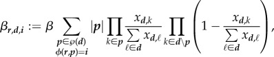4.3

where β is the constant transmission factor, is the sum over all possible inocula of host d that turn host r into host i, |p| is the rank of the inoculum class (number of genotypes), 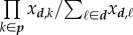is the product of genotype frequencies in d over all genotypes of p, and 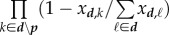is conversely the product of the complementary frequencies over the remaining genotypes of d.

Importantly, β_r,d,i is an infection rate and not a transmission rate, as it quantifies the flow between two host compartments due to infection. In models that consider only one kind of host that can be infected, S, and only one kind of infected host (I), there is only one infection rate, β (and βSI is the infection flow) [15]. This infection rate is then also the transmission rate because there is only one host class that can be infected (S) and because infection always leads to the same host class (I). The infection rate–transmission rate equality still holds in more complex models with several infected host types if genotypes are transmitted one at a time [21,34]. In our model of transmission, however, donor hosts can cotransmit any subset of their co-infecting genotype combination, whereas receiver hosts may not be affected by such contacts or may be affected differently according to within-host parameters. Infection flows are thus unpredictable here because they depend, through the infection operator ϕ, on the outcomes of the within-host dynamics, which determine how steady-state parasite loads are affected by contamination of new genotypes. Because ODEs (4.1) and (4.2) only describe flows between compartments, β_r,d,i refers to infection rates and not to more intuitive transmission rates.

Nonetheless, it is possible to make an interpretation of the transmission process based on the definition of β_r,d,i. To do so, one should consider that transmission is a process that does not depend on the outcome of the contamination (which becomes an infection event only if the receiver host class changes). In other words, if we denote by β_d, the overall transmission rate of infected host class d, β_r,d,i gives β_d when ignoring the condition ϕ(r, p) = i under the sum or when assuming that all the inocula classes p of d are epidemiological.

In the case where we assume that all the inocula classes of the donor host class d are epidemiological, ϕ (∅︀, p) = p for all p ∈ ℘(d)^★ and β_d is measured as the overall transmission rate to a susceptible, that is .

Subsequently, it is possible to define the rate at which a given genotype k is transmitted by hosts from class d. We denote this rate β_d,k. We show in the electronic supplementary material, appendix D.1, that

4.4

as expected, but also that

4.5

As a consequence, the transmission rate of a host does not depend either on the total parasite load nor on the number of infecting genotypes. For a given genotype, a higher parasite load confers no transmission advantage in single infections for a given genotype but it does confer an advantage in co-infections because the probability of being transmitted increases with its frequency. Transmission rates of co-infected hosts thus reflect the outcome of the within-host dynamics.

(ii). Recovery rates

Recovery rates are the rate at which hosts d turn into hosts i through recovery,

4.6

where θ is the constant recovery factor, and 1 is the number of genotypes that make class d hosts to reach class i through a recovery event. Note that the condition implies that is an epidemiological class.

For a given couple of host classes (d, i) ∈ ℰ^★ × ℰ, recovery is thus interpreted as a constant rate θ multiplied by the number of ways a class d host can recover and turn into a class i host. This is also the number of genotypes the recovery from which leads the parasite loads to the steady-state . This number is greater than one if and only if several genotypes cannot survive in the co-infection without the presence of each other.

The total recovery rate of a given infected host class d is |d|θ as recovering from a genotype always leads to another host class.

(iii). Death rates

The death rates are given as the sum over all parasite loads times a constant death factor,

4.7

Death rates are assumed to be linear functions of the total parasite load: the higher the parasite load a host carries, the more rapidly it dies. Total parasite load can therefore be used as a proxy for virulence.

(d). Synthesis

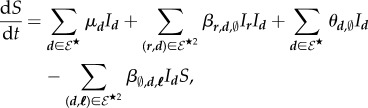
The following master equation captures the between-host dynamics:

4.8

where is the infection input flow matrix, is the infection output flow matrix, is the recovery input flow matrix, Θ is the recovery output flow matrix and Δ is the death matrix. There is no general expression for these matrices because their structure depends on the way classes are ordered. For an explicit definition of these matrices according to the labelling we use for computing the model, see the electronic supplementary material, appendix D.2.

Although equation (4.8) cannot be solved analytically, it is a useful expression of the between-host dynamics that allows for fast computing.

Between-host dynamics are summarized in figure 2.

Figure 2.

Between-host flow diagram focused on host class i, represented here as a set of five out of n = 10 genotypes. Not all the flows involving are shown but each type of event is shown at least once. The rates are given as they appear in the ODE satisfied by . The matrix through which each flow is introduced into the master equation is shown in brackets. The solid filled triangle-ended arrows stand for infection flows and are joined by dashed lines that indicate the donor. The solid hollow square-ended arrows stand for recovery flows. While a host can be infected by several genotypes simultaneously, it recovers only from one genotype at a time. The dot-ended arrow followed by a dotted arrow represents the death flow that leads to the susceptible compartment, as a consequence of the constant population size assumption.

5. Basic reproduction numbers and epidemiological feedback

The basic reproduction number, denoted by ℛ₀, is the most widely used parameter in epidemiological modelling [14,34,35]. ℛ₀ is defined as the expected number of secondary infections produced by a single infected individual during its entire period of infectiousness in a fully susceptible population [28,36,37]. Hence, it is often interpreted as the fitness of the parasite [15,38,39] or as the inverse of the minimum proportion of vaccinated hosts required to eradicate an infectious disease [37]. More generally, ℛ₀ corresponds to the epidemiological threshold above which the endemic state is always reached (i.e. when ℛ₀ > 1).

The latest and most general method to determine the basic reproduction number relies on the asymptotic instability of the disease-free equilibrium [40,41], that is to say ℛ₀ greater than 1 if and only if the between-host steady state where all hosts are susceptibles is unstable. This method, called ‘next-generation’, is usually convenient because it does not require finding the infected steady-state densities. On the other hand, it may not provide any information on the proportion of susceptible or infected hosts at the infected steady state. According to the instability of the ‘disease-free equilibrium’, the ‘next-generation basic reproduction number’ of our model is

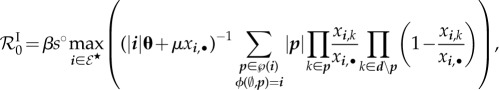5.1

where • stands for the sum over the given index (see proof in electronic supplementary material, appendix E.1).

Other methods calculate ℛ₀ via the positivity condition of the infected steady-state density [42,43]. In this case ℛ₀ is simply the inverse of the proportion of the remaining susceptibles [44]. If we call J the sum of the infected hosts densities, we have which gives the following ‘endemic basic reproduction number’

5.2

This quantity can be written in our model as a function of the steady-state marginal arithmetic means of infection, recovery and death rates, as

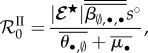5.3

where the marginal arithmetic means over one and two indices are, respectively, denoted by 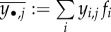and 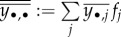(see proof in the electronic supplementary material, appendix E.2).

These two basic reproduction numbers share two important features.

First, like the basic reproduction number of simple models (such as SIS and SIR), they are the ratio of a transmission factor in a fully susceptible host population over a sum of recovery and death rates. This is classically interpreted as the expected number of secondary infected hosts at the beginning of an epidemic, where there is only one infected host (as the transmission rate is multiplied by the infected host life expectancy).

Second, ℛ₀ > 1 means that there is at least one infected compartment that is non-zero at steady state. This does not provide any information, however, on which host class and parasite genotype is involved in the endemic.

However, unlike the next-generation basic reproduction number (), the rates involved in the endemic basic reproduction number () are arithmetic means that depend on the distribution of host class frequencies at steady state. Therefore, it is possible for to show complex behaviours when epidemiological parameters vary.

Because between-host dynamics are nonlinear, changes in epidemiological parameters that determine the rates of epidemiological events can cause non-trivial modifications of the steady state. These are often referred to as epidemiological feedbacks [13]. We prove in the electronic supplementary material, appendix E.3, that the endemic basic reproduction number can capture these while the next-generation basic reproduction number cannot. This is also illustrated in figure 3.

Figure 3.

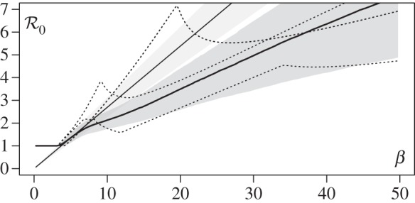
Apprehending epidemiological feedbacks through the endemic basic reproduction number. Considering five parasite genotypes (n = 5), 300 within-host parameter sets were randomly generated (see below) and 200 epidemic simulations were ran with each parameter set by varying the transmission factor β from 0 to 50. The constant recovery and death factors were fixed (μ = 5 and θ = 3). The initial density of infected hosts was set to 10⁻³s°, equally distributed to all the epidemiological host classes. Both basic reproduction numbers were calculated according to equations (5.1) and (5.2) for each run. was also numerically derived twice with respect to β. Over all parameter sets and all values of β, the standard deviation of is about 0.11 and the maximum is about 3.94. The figure shows the mean of (thin solid line) and (thick solid line) as a function of β over the 300 parameter sets, along their standard deviation (respectively, the light grey area and the dark grey area). The of three particular parameter sets (dotted lines) are also given as examples of strong epidemiological feedbacks. The within-host parameters were drawn in the standard uniform distribution 𝒰(0,1), excepted for η_ij, i ≠ j, drawn in 𝒰(−1, 1) and η_i,i was calculated as with drawn in 𝒰(0, 1). The standard clearing rate υ was fixed to 1.

Our simulations in figure 3 show that is a nonlinear function of intermediate values of β (even after averaging over hundreds of parameter sets), confirming that it captures epidemiological feedbacks. Moreover, individual parameter combinations (dotted lines) often exhibit local minima of . Therefore, any increase or decrease in β starting from this minimum will increase the steady-state total prevalence of infection. This means that public health interventions that decrease transmission could increase disease spread or, conversely, that factors increasing contact rate between hosts could slow down disease spread. This unexpected effect is correlated with genotypic diversity, as the median of is −3.33 × 10⁻² for the n = 5 results shown in figure 3 and −1.05 × 10⁻⁵ in similar simulations done for n = 2 (not shown).

To understand the phenomenon that leads to the nonlinearities in , it helps to consider the case of two genotypes that can co-infect the same host. When β is hardly large enough for (and ) to be greater than one, the genotype with the lowest parasite load in single infections is the only one that becomes endemic. The second genotype is epidemiologically cleared because it kills hosts faster, such that its proper basic reproduction number is lower than one (recall that transmission does not increase with parasite load in single infection). When β is large enough to compensate for the higher death rate induced by the second genotype, this genotype also spreads in the host population. Susceptible hosts are turned into singly infected hosts at first, but as the two genotypes can co-infect the same host, both singly infected host classes infect one another and become co-infected hosts. Nonlinearities can then appear if the total parasite load of the co-infected host is greater than the parasite load of the singly infected. Indeed, some of the singly infected hosts become co-infected and then die more rapidly than if they had remained singly infected, so the basic reproduction number decreases, even if β has increased. Note that our model shows coexistence of parasite genotypes not over the evolutionary time scale between singly infected hosts, as shown in previous sutdies [25,45], but over the epidemic time scale with the persistence of co-infected hosts.

An analoguous reasoning can be done in the case of superinfection. As above, the genotype with the highest parasite load in single infections spreads in the population already infected by the first genotype only if β is large enough so it compensates the higher death rate of its singly infected hosts. Nonlinearities can then appear if the second genotype superinfects the first-genotype-infected hosts. Some of the latter hosts become infected by the second genotype and die more rapidly than if they had remained infected by the first genotype. Again decreases, even though β has increased.

If nonlinearity is possible for only two genotypes, it is even more favoured for a higher number of genotypes because the infection patterns can be a combination of superinfections and co-infections, thus multiplying the sources of nonlinearity.

6. Discussion

There is a crying lack of general models for multiple infections. The few exceptions that allow for more than two parasite genotypes rely on very stringent assumptions [19,21]. Here, we introduce a novel model with many potentialities. Above all, it can include any number of unrelated different parasite genotypes, whereas the vast majority of existing models are restricted to a single monomorphic parasite, or few related parasites. Our model also brings new features to infectious diseases modelling.

The first feature is the explicit modelling of diverse within-host dynamics, where the host plays the role of an isolated constant ecosystem in which parasites grow. As in population dynamics [29] and multispecies ecological models [46,47], the growth rate of each parasite genotype is affected by its own density and the density of the other genotypes. PPs (PGs and spite) are also taken into account through their own proper dynamics. Along with parasite-load-dependent effects, PPs enrich the diversity of within-host dynamics and outcomes. Although PGs and spite have already been integrated in within-host dynamics [10,20,48], they have never been included together and linked with an epidemiological model, while it is known that some parasites can produce both PGs and spite with epidemiological consequences [23]. Our model can also integrate additional interactions, especially competition for host resources, host immune response and cross-immunity through the parasite-load-dependent effects.

Nested dynamics have already been tackled [12,27], but have never been generalized to several within-host interactions and for more than two parasite genotypes. This flexibility generates a great diversity of infection patterns which increases exponentially, as the number of parasite combinations, with the number of considered genotypes.

In particular, linking the two levels allows us to identify a biological scenario that the superinfection and the co-infection hypotheses fail to capture. This occurs when genotype combinations are unstable and cause unlimited growth. Indeed, while several genotypes can grow inside the host (as in co-infections), the host may vanish at the host population level (as in superinfections) because of infinite death rate. We call such a pattern ultrainfection.

A second new feature is the set of definitions of biological and epidemiological classes for hosts and inocula. These definitions allow us to build functions to go beyond the classical superinfection–co-infection dichotomy [18,19] which has proved to be problematic [26]. A final original feature of the between-host part of the model allows for partial cotransmission, that is an infected host can infect another host with any subset of its co-infecting genotypes combination, unlike the other multiple infection models that assume sequential or all-or-nothing transmission (but see [49]).

Epidemiological feedbacks drive between-host outcomes [34] and selective pressures [13]. Despite the complexity of our model, we show that it is possible to capture these feedbacks through the endemic basic reproduction number (see also [36]). As shown in figure 3, in some situations, the basic reproduction number, and thus disease prevalence, can increase even if the transmission factor decreases, because of the multiplicity of genotypes. This effect is missed by methods that are based on the next-generation basic reproduction number [50] because it is equal to the endemic basic reproduction number when only one genotype is considered (see the electronic supplementary material, appendix E.4). Overlooking parasite genotypic diversity can therefore have major consequences, as quarantine measures could, for instance, increase disease spread instead of preventing it. Overall, we argue that accounting for parasite genotypic diversity and using the endemic basic reproduction number to study epidemiological feedbacks is key to controlling infectious diseases.

As this is the first analysis of this multi-strain multiple infection model, we had to make some simplifying assumptions. Some of these, such as the time-scale separation, are constitutive of the model but others could be alleviated or modified. In particular, the assumptions linking within-host steady-state variables (population sizes) to epidemiological parameters (transmission rate, virulence and recovery rate) can be changed without affecting the between-host master equation. This is important as these assumptions are likely to depend on the biological system considered. Here, we assumed the transmission rate to be constant, which has the advantage that the only selective pressure allowing the persistence of virulent parasites has to come from the within-host level. Further extensions of this model could consider a link between parasite load and transmission rate. However, earlier models have shown that further assumptions would then be needed because if both virulence and transmission rates are linear functions of parasite load, natural selection will always favour the strains with the highest possible level of virulence [51]. One possibility could be to focus on a biological system where these relationships have been parametrized, such as HIV in humans [52], myxomatosis in rabbits [53], Ophryocystis elektroscirrha in monarch butterflies [54] or the cauliflower mosaic virus in turnips [55].

The between-host dynamics used here are also based on simplifying assumptions that may not be suitable for all host–parasite systems: time-scale separation, random mixing, host homogeneity, lack of immunization and constant population size, range from the strongest and hardest to adapt from the given equations to the weakest and easy to relax.

Finally, a direct application of this model has to do with parameter inference. Indeed, for many diseases, we have detailed epidemiological data on the prevalence of co-infections that include combinatorial diversity (for instance in the case of human papillomavirus [56]). Such data, possibly combined with information on within-host processes, could allow us to compare between models and estimate parameters.

Overall, our model opens new perspectives for investigating the evolution of parasite traits such as virulence and PGs and spite production rates in multiple infections owing to its capacity for handling the combinatorial complexity of cotransmissions and epidemiological feedbacks.

Authors' contributions

M.T.S., S.A. and Y.M. conceived the project, M.T.S. performed the analysis, and M.T.S., S.A. and Y.M. wrote the article.

Competing interests

We have no competing interests.

Funding

M.T.S., S.A. and Y.M. acknowledge support from the CNRS, the UM and the IRD. S.A. is supported by an ATIP-Avenir.

References

- 1.Petney TN, Andrews RH. 1998. Multiparasite communities in animals and humans: frequency, structure and pathogenic significance. Int. J. Parasitol. 28, 377–393. ( 10.1016/S0020-7519(97)00189-6) [DOI] [PubMed] [Google Scholar]
- 2.Lord C, Barnard B, Day K, Hargrove J, McNamara J, Paul R, Trenholme K, Woolhouse MEJ. 1999. Aggregation and distribution of strains in microparasites. Phil. Trans. R. Soc. Lond. B 354, 799–807. ( 10.1098/rstb.1999.0432) [DOI] [PMC free article] [PubMed] [Google Scholar]
- 3.Juliano JJ, Porter K, Mwapasa V, Sem R, Rogers WO, Ariey F, Wongsrichanalai C, Read A, Meshnick SR. 2010. Exposing malaria in-host diversity and estimating population diversity by capture-recapture using massively parallel pyrosequencing. Proc. Natl Acad. Sci. USA 107, 20 138–20 143. ( 10.1073/pnas.1007068107) [DOI] [PMC free article] [PubMed] [Google Scholar]
- 4.Balmer O, Tanner M. 2011. Prevalence and implications of multiple-strain infections. Lancet Infect. Dis. 11, 868–878. ( 10.1016/S1473-3099(11)70241-9) [DOI] [PubMed] [Google Scholar]
- 5.Raso G, et al. 2004. Multiple parasite infections and their relationship to self-reported morbidity in a community of rural Côte d'Ivoire. Int. J. Epidemiol. 33, 1092–1102. ( 10.1093/ije/dyh241) [DOI] [PubMed] [Google Scholar]
- 6.Bentwich Z, Kalinkovich A, Weisman Z, Borkow G, Beyers N, Beyers AD. 1999. Can eradication of helminthic infections change the face of AIDS and tuberculosis? Immunol. Today 20, 485–487. ( 10.1016/S0167-5699(99)01499-1) [DOI] [PubMed] [Google Scholar]
- 7.Brown SP, Grenfell BT. 2001. An unlikely partnership: parasites, concomitant immunity and host defence. Proc. R. Soc. Lond. B 268, 2543–2549. ( 10.1098/rspb.2001.1821) [DOI] [PMC free article] [PubMed] [Google Scholar]
- 8.Mideo N. 2009. Parasite adaptations to within-host competition. Trends Parasitol. 25, 261–268. ( 10.1016/j.pt.2009.03.001) [DOI] [PubMed] [Google Scholar]
- 9.Kümmerli R, Brown SP. 2010. Molecular and regulatory properties of a public good shape the evolution of cooperation. Proc. Natl Acad. Sci. USA 107, 18 921–18 926. ( 10.1073/pnas.1011154107) [DOI] [PMC free article] [PubMed] [Google Scholar]
- 10.West SA, Buckling A. 2003. Cooperation, virulence and siderophore production in bacterial parasites. Proc. R. Soc. Lond. B 270, 37–44. ( 10.1098/rspb.2002.2209) [DOI] [PMC free article] [PubMed] [Google Scholar]
- 11.Riley MA, Wertz JE. 2002. Bacteriocins: evolution, ecology, and application. Annu. Rev. Microbiol. 56, 117–137. ( 10.1146/annurev.micro.56.012302.161024) [DOI] [PubMed] [Google Scholar]
- 12.Choisy M, de Roode JC. 2010. Mixed infections and the evolution of virulence: effects of resource competition, parasite plasticity, and impaired host immunity. Am. Nat. 175, E105–E118. ( 10.1086/651587) [DOI] [PubMed] [Google Scholar]
- 13.Alizon S, de Roode JC, Michalakis Y. 2013. Multiple infections and the evolution of virulence. Ecol. Lett. 16, 556–567. ( 10.1111/ele.12076) [DOI] [PubMed] [Google Scholar]
- 14.Kermack WO, McKendrick AG. 1932. Contributions to the mathematical theory of epidemics. II. The problem of endemicity. Proc. R. Soc. Lond. A 138, 55–83. ( 10.1098/rspa.1932.0171) [DOI] [Google Scholar]
- 15.Anderson R, May R. 1982. Coevolution of hosts and parasites. Parasitology 85, 411–426. ( 10.1017/S0031182000055360) [DOI] [PubMed] [Google Scholar]
- 16.Levin S, Pimentel D. 1981. Selection of intermediate rates of increase in parasite–host systems. Am. Nat. 117, 308–315. ( 10.1086/283708) [DOI] [Google Scholar]
- 17.van Baalen M, Sabelis MW. 1995. The dynamics of multiple infection and the evolution of virulence. Am. Nat. 146, 881–910. ( 10.1086/285830) [DOI] [Google Scholar]
- 18.Nowak MA, May RM. 1994. Superinfection and the evolution of parasite virulence. Proc. R. Soc. Lond. B 255, 81–89. ( 10.1098/rspb.1994.0012) [DOI] [PubMed] [Google Scholar]
- 19.May RM, Nowak MA. 1995. Coinfection and the evolution of parasite virulence. Proc. R. Soc. Lond. B 261, 209–215. ( 10.1098/rspb.1995.0138) [DOI] [PubMed] [Google Scholar]
- 20.Brown SP, Hochberg ME, Grenfell BT. 2002. Does multiple infection select for raised virulence? Trends Microbiol. 10, 401–405. ( 10.1016/S0966-842X(02)02413-7) [DOI] [PubMed] [Google Scholar]
- 21.Lion S. 2013. Multiple infections, kin selection and the evolutionary epidemiology of parasite traits. J. Evol. Biol. 26, 2107–2122. ( 10.1111/jeb.12207) [DOI] [PubMed] [Google Scholar]
- 22.de Roode JC, Helinski ME, Anwar MA, Read AF. 2005. Dynamics of multiple infection and within-host competition in genetically diverse malaria infections. Am. Nat. 166, 531–542. ( 10.1086/491659) [DOI] [PubMed] [Google Scholar]
- 23.Garbutt J, Bonsall MB, Wright DJ, Raymond B. 2011. Antagonistic competition moderates virulence in Bacillus thuringiensis. Ecol. Lett. 14, 765–772. ( 10.1111/j.1461-0248.2011.01638.x) [DOI] [PubMed] [Google Scholar]
- 24.Bremermann HJ, Pickering J. 1983. A game-theoretical model of parasite virulence. J. Theor. Biol. 100, 411–426. ( 10.1016/0022-5193(83)90438-1) [DOI] [PubMed] [Google Scholar]
- 25.Boldin B, Diekmann O. 2008. Superinfections can induce evolutionarily stable coexistence of pathogens. J. Math. Biol. 56, 635–672. ( 10.1007/s00285-007-0135-1) [DOI] [PubMed] [Google Scholar]
- 26.Alizon S, van Baalen M. 2008. Multiple infections, immune dynamics, and the evolution of virulence. Am. Nat. 172, E150–E168. ( 10.1086/590958) [DOI] [PubMed] [Google Scholar]
- 27.Mideo N, Alizon S, Day T. 2008. Linking within- and between-host dynamics in the evolutionary epidemiology of infectious diseases. Trends Ecol. Evol. 23, 511–517. ( 10.1016/j.tree.2008.05.009) [DOI] [PubMed] [Google Scholar]
- 28.Anderson RM, May RM. 1991. Infectious diseases of humans, vol. 1 Oxford, UK: Oxford University Press. [Google Scholar]
- 29.Verhulst PF. 1838. Notice sur la loi que la population suit dans son accroissement. Correspondance Mathématique et Physique Publiée par A. Quetelet 10, 113–121. [Google Scholar]
- 30.Neilands J. 1995. Siderophores: structure and function of microbial iron transport compounds. J. Biol. Chem. 270, 26 723–26 726. ( 10.1074/jbc.270.45.26723) [DOI] [PubMed] [Google Scholar]
- 31.Gardner A, West SA, Buckling A. 2004. Bacteriocins, spite and virulence. Proc. R. Soc. Lond. B 271, 1529–1535. ( 10.1098/rspb.2004.2756) [DOI] [PMC free article] [PubMed] [Google Scholar]
- 32.Andreasen V, Lin J, Levin SA. 1997. The dynamics of cocirculating influenza strains conferring partial cross-immunity. J. Math. Biol. 35, 825–842. ( 10.1007/s002850050079) [DOI] [PubMed] [Google Scholar]
- 33.Kermack WO, McKendrick AG. 1927. A contribution to the mathematical theory of epidemics. Proc. R. Soc. Lond. A 115, 700–721. ( 10.1098/rspa.1927.0118) [DOI] [Google Scholar]
- 34.Alizon S. 2013. Co-infection and super-infection models in evolutionary epidemiology. Interface Focus 3, 20130031 ( 10.1098/rsfs.2013.0031) [DOI] [PMC free article] [PubMed] [Google Scholar]
- 35.Anderson RM, May RM. 1979. Population biology of infectious diseases: part I. Nature 280, 361–367. ( 10.1038/280361a0) [DOI] [PubMed] [Google Scholar]
- 36.Diekmann O, Heesterbeek J, Metz JA. 1990. On the definition and the computation of the basic reproduction ratio R0 in models for infectious diseases in heterogeneous populations. J. Math. Biol. 28, 365–382. ( 10.1007/BF00178324) [DOI] [PubMed] [Google Scholar]
- 37.Diekmann O, Heesterbeek J. 2000. Mathematical epidemiology of infectious diseases: model building, analysis, and interpretation. New York, NY: Wiley. [Google Scholar]
- 38.Alizon S, Hurford A, Mideo N, van Baalen M. 2009. Virulence evolution and the trade-off hypothesis: history, current state of affairs and the future. J. Evol. Biol. 22, 245–259. ( 10.1111/j.1420-9101.2008.01658.x) [DOI] [PubMed] [Google Scholar]
- 39.Alizon S, Michalakis Y. 2015. Adaptive virulence evolution: the good old fitness-based approach. Trends Ecol. Evol. 30, 248–254. ( 10.1016/j.tree.2015.02.009) [DOI] [PubMed] [Google Scholar]
- 40.Van den Driessche P, Watmough J. 2002. Reproduction numbers and sub-threshold endemic equilibria for compartmental models of disease transmission. Math. Biosci. 180, 29–48. ( 10.1016/S0025-5564(02)00108-6) [DOI] [PubMed] [Google Scholar]
- 41.Hurford A, Cownden D, Day T. 2009. Next-generation tools for evolutionary invasion analyses. J. R. Soc. Interface 7, 561–571. ( 10.1098/rsif.2009.0448) [DOI] [PMC free article] [PubMed] [Google Scholar]
- 42.Heffernan J, Smith R, Wahl L. 2005. Perspectives on the basic reproductive ratio. J. R. Soc. Interface 2, 281–293. ( 10.1098/rsif.2005.0042) [DOI] [PMC free article] [PubMed] [Google Scholar]
- 43.Roberts M. 2007. The pluses and minuses of R0. J. R. Soc. Interface 4, 949–961. ( 10.1098/rsif.2007.1031) [DOI] [PMC free article] [PubMed] [Google Scholar]
- 44.Dietz K, Schenzle D. 1985. Proportionate mixing models for age-dependent infection transmission. J. Math. Biol. 22, 117–120. ( 10.1007/BF00276550) [DOI] [PubMed] [Google Scholar]
- 45.Pugliese A. 2002. On the evolutionary coexistence of parasite strains. Math. Biosci. 177, 355–375. ( 10.1016/S0025-5564(02)00083-4) [DOI] [PubMed] [Google Scholar]
- 46.Lotka AJ. 1925. Elements of physical biology. Baltimore, MD: Williams and Wilkins. [Google Scholar]
- 47.Volterra V. 1928. Variations and fluctuations of the number of individuals in animal species living together. ICES J. Mar. Sci. 3, 3–51. ( 10.1093/icesjms/3.1.3) [DOI] [Google Scholar]
- 48.Buckling A, Brockhurst M. 2008. Kin selection and the evolution of virulence. Heredity 100, 484–488. ( 10.1038/sj.hdy.6801093) [DOI] [PubMed] [Google Scholar]
- 49.Alizon S. 2013. Parasite co-transmission and the evolutionary epidemiology of virulence. Evolution 67, 921–933. ( 10.1111/j.1558-5646.2012.01827.x) [DOI] [PubMed] [Google Scholar]
- 50.Anderson R, May R. 1983. Vaccination against rubella and measles: quantitative investigations of different policies. J. Hyg. 90, 259–325. ( 10.1017/S002217240002893X) [DOI] [PMC free article] [PubMed] [Google Scholar]
- 51.Alizon S, van Baalen M. 2005. Emergence of a convex trade-off between transmission and virulence. Am. Nat. 165, E155–E167. ( 10.1086/430053) [DOI] [PubMed] [Google Scholar]
- 52.Fraser C, Hollingsworth TD, Chapman R, de Wolf F, Hanage WP. 2007. Variation in HIV-1 set-point viral load: epidemiological analysis and an evolutionary hypothesis. Proc. Natl Acad. Sci. USA 104, 17 441–17 446. ( 10.1073/pnas.0708559104) [DOI] [PMC free article] [PubMed] [Google Scholar]
- 53.Dwyer G, Levin SA, Buttel L. 1990. A simulation model of the population dynamics and evolution of myxomatosis. Ecol. Monogr. 60, 423–447. ( 10.2307/1943014) [DOI] [Google Scholar]
- 54.de Roode JC, Yates AJ, Altizer S. 2008. Virulence-transmission trade-offs and population divergence in virulence in a naturally occurring butterfly parasite. Proc. Natl Acad. Sci. USA 105, 7489–7494. ( 10.1073/pnas.0710909105) [DOI] [PMC free article] [PubMed] [Google Scholar]
- 55.Doumayrou J, Avellan A, Froissart R, Michalakis Y. 2013. An experimental test of the transmission-virulence trade-off hypothesis in a plant virus. Evolution 67, 477–486. ( 10.1111/j.1558-5646.2012.01780.x) [DOI] [PubMed] [Google Scholar]
- 56.Garland SM, Steben M, Sings HL, James M, Lu S, Railkar R, Barr E, Haupt RM, Joura EA. 2009. Natural history of genital warts: analysis of the placebo arm of 2 randomized phase III trials of a quadrivalent human papillomavirus (types 6, 11, 16, and 18) vaccine. J. Infect. Dis. 199, 805–814. ( 10.1086/597071) [DOI] [PubMed] [Google Scholar]
Associated Data
This section collects any data citations, data availability statements, or supplementary materials included in this article.