Introduction of a new critical p value correction method for statistical significance analysis of metabonomics data

Abstract

Nuclear magnetic resonance (NMR) spectroscopy-based metabonomics is of growing importance for discovery of human disease biomarkers. Identification and validation of disease biomarkers using statistical significance analysis (SSA) is critical for translation to clinical practice. SSA is performed by assessing a null hypothesis test using a derivative of the Student’s t test, e.g., a Welch’s t test. Choosing how to correct the significance level for rejecting null hypotheses in the case of multiple testing to maintain a constant family-wise type I error rate is a common problem in such tests. The multiple testing problem arises because the likelihood of falsely rejecting the null hypothesis, i.e., a false positive, grows as the number of tests applied to the same data set increases. Several methods have been introduced to address this problem. Bonferroni correction (BC) assumes all variables are independent and therefore sacrifices sensitivity for detecting true positives in partially dependent data sets. False discovery rate (FDR) methods are more sensitive than BC but uniformly ascribe highest stringency to lowest p value variables. Here, we introduce standard deviation step down (SDSD), which is more sensitive and appropriate than BC for partially dependent data sets. Sensitivity and type I error rate of SDSD can be adjusted based on the degree of variable dependency. SDSD generates fundamentally different profiles of critical p values compared with FDR methods potentially leading to reduced type II error rates. SDSD is increasingly sensitive for more concentrated metabolites. SDSD is demonstrated using NMR-based metabonomics data collected on three different breast cancer cell line extracts.

Introduction

Nuclear magnetic resonance (NMR) spectroscopy is widely used in metabonomics for discovery of potential biomarkers of human diseases [1, 2]. While high-resolution NMR spectroscopy provides rich information of human urine, serum, cell lines, and so on [3], it also generates large data sets, which when combined with inter-individual variations, significantly increases data analysis complexity [4]. Hence, there is continuing development of data reduction methods to facilitate biomarker discovery and validation. In the past two decades, projection methods such as principal components analysis (PCA) [5, 6] and partial least squares discriminant analysis (PLS-DA) [7, 8] have been used frequently to facilitate interpretation of metabonomics data. PCA provides a visual overview of the data making it easier to detect clustering patterns and data outliers, whereas PLS-DA is intended for model building and classification. Orthogonal signal correction PLS-DA (O-PLS-DA) has been introduced to filter noise uncorrelated between case and control samples [9]. In these projection methods, score and loading plots are generated to allow visual assessment of data. The scores plot represents the similarity relationship between spectra, with similar spectra clustering in the principal component space, whereas the loadings plot indicates the contribution that each variable (e.g., NMR peak) makes to group separation in the scores plot [10]. The variables with the largest loadings indicate potential metabolic biomarkers for human diseases. The first step in validating the importance of metabolites identified from the loadings plot is to determine if the differences in metabolite concentrations between populations are statistically significant. Thus, statistical significance analysis (SSA) of PCA and PLS-DA loadings data are critical to metabolomics-based biomarker discovery and validation and translation to clinical use.

PCA and PLS-DA loadings and scores can be affected significantly by data scaling pretreatment [2] as this process affects the variance/covariance matrix, and the eigenvectors and eigenvalues obtained from diagonalization of the variance/covariance matrix ultimately determine the scores and loadings. Three data pretreatment scaling methods are mainly used in NMR-based metabonomics studies [11]. No scaling is often used as NMR peak intensities are directly comparable. No scaling tends to give more weight to the variance/covariance of the strongest NMR peaks compared with variations in the weaker NMR peaks. Auto scaling, i.e., scaling to unit variance, calculated by division of the difference of the mean-centered variable intensities by the pooled standard deviations, is intended to be used either when variables are not directly comparable, or when there is no prior knowledge about the relative importance of the variables. While auto scaling gives equal importance to all variables regardless of their prominence in the data set, i.e., weak peaks are given equal weight to strong peaks, it sacrifices information about relative metabolite concentrations. PLS-DA and statistical total correlation spectroscopy (STOCSY) [12] are based on auto scaling. STOCSY, designed for identification of peaks belonging to the same metabolite and for detecting correlated changes in metabolite concentrations, relies on calculation of Pearson correlation coefficients between variables, which can introduce higher than expected correlation noise making it sometimes difficult to interpret the results [13]. Pareto scaling, in which centered data are divided by the square root of the standard deviation, is a compromise between no scaling and auto scaling, where variations of weaker features in the data are given more weight relative to stronger features compared with no scaling data pretreatment.

In PLS-DA, it is standard to pre-process raw data by mean centering followed by auto scaling prior to calculating the variance/covariance matrix. Consequently, the differences between the observed variable intensity and the mean variable intensities (actually the integrated areas of each variable or “bucket”) are divided by the pooled bucket intensity standard deviations [14, 15]. This data pretreatment step results in unit variance for each variable or bucket, and as a result, information regarding the relative variance and relative intensities of the variables are lost as the magnitude of the standard deviation tends to correlate with variable intensity [14, 16]. Although auto scaling is standard for PLS-DA, it has become common to plot the magnitude of each variable loading multiplied by its corresponding standard deviation at each variable frequency to restore relative metabolite concentration information. The loadings for each variable are then scaled to a maximum value of one and used to generate a heat map with values ranging from 0 to 1, and the peaks in the resulting PLS-DA spectrum are color coded according to this heat map. A threshold value is selected from this heat map, which is based on the variable loadings, as a cutoff to identify important variables. We refer to this manner of presentation of PLS-DA as adjusted PLS-DA (aPLS-DA). In general, PLS-DA is used for model building and classification. A limitation of PLS-DA data presentation is that the loadings are not subjected to SSA.

SSA depends on null hypothesis testing, typically with the use of a modified Student’s t test, e.g., a Welch’s t test. The null hypothesis states that there is no difference between the means of two groups of measurements. Application of the t test requires definition of a significance level, α, which is used as a criterion to reject the null hypothesis. A typical value of α is 0.05, meaning that there will be no more than a 5 % probability that a true null hypothesis will be falsely rejected. This type of error is referred to as a type I error, which leads to a false positive relationship. Stated alternatively, an α value equal to 0.05 corresponds to a 95 % confidence level in accurately rejecting a false null hypothesis. The t test generates a test statistic that is converted into a p value, and if the p value is less than the significance level, the null hypothesis can be rejected. However, when multiple tests are conducted on the same data set, the probability of a type I error occurring increases. To ensure a constant family-wise type I error rate, various methods have been introduced to correct the critical p value that must be applied to preserve the desired significance level for all simultaneous inferences made across the entire data set [17, 18]. The most conservative approach is the Bonferroni correction (BC) which assumes that all the variables in the data set are independent [19–21], and as a result, BC sacrifices sensitivity if the variables in the data set are not truly independent. In metabonomics studies, it is possible for NMR peaks to vary dependently either when the resonances belong to the same metabolites or when they belong to metabolites that share a common biochemical pathway, in either case, invalidating the independent variable hypothesis. In the case of partially dependent data sets, too-conservative application of a multiple testing correction can lead to type II errors, i.e., false negatives. In such cases, which will essentially always be the case for NMR-based metabonomics studies, alternative methods for correcting for multiple simultaneous testing must be applied to avoid type II errors. False discovery rate (FDR) methods like Benjamini–Hochberg FDR (BH-FDR) [22] or Benjamini–Yekutieili FDR (BY-FDR) [23] were developed to reduce type II error rates, and as a result are more sensitive and less conservative than BC. In PLS-DA, p values are not calculated; alternatively, a quantity called variable importance (VIP) has been introduced to analyze PLS-DA loadings, which reflects the influence of every term (x_k) in the model on the Y matrix. VIP values larger than one are considered important (user tutorial of SIMCA-P+(v.11), Umetrics) [24]. The method was not designed to control type I or II error but arbitrarily establishes a cut off for the PLS-DA loadings. However, none of these methods gives weight to metabolite concentration information, which may be a potentially important consideration for some clinical applications.

Here, we introduce a new method for correcting the critical p value threshold used for SSA in the case of multiple testing in partially dependent data sets. We refer to the new method as standard deviation step down (SDSD). The new SDSD method is more sensitive and less conservative than BC and allows for adjustment and refinement to improve sensitivity while reducing type II error rate depending on the anticipated or measured fraction of dependent variables in the data set. The SDSD method takes into account relative metabolite concentration information, placing progressively more importance on the strongest features in a data set, similar to PCA with no scaling, but with greater sensitivity. SDSD, compared with other existing methods, results in a fundamentally different profile of variable critical p values. Whereas FDR and Holm’s procedures utilize rank order of p values as a step down scale factor, ensuring that the smallest p value variables are subjected to the most stringent critical p value threshold, the SDSD step down factor is based on rank order of standard deviations, and therefore there is no strict relationship between raw p value and assigned stringency, potentially leading to reduced type II error rates, i.e., false negatives. The SDSD method is demonstrated using NMR-based metabolic profiling data collected on cell extracts from three distinct breast cancer cell lines, as described below. The new method can also be applied to other techniques with large numbers of variables, such as liquid chromatography–mass spectrometry (LC-MS)-based metabonomic data sets.

Experimental section

Materials and methods: data collection and processing

Three different modified MCF-7 breast cancer cell lines were used to test the new SDSD correction method. MCF-7 cells transfected with genes encoding the splice variants osteopontin-A (A) or osteopontin-C (C) were used as case groups, and MCF-7 cells transfected with an empty vector (V) were used as a control group [25]. Six samples were prepared from each group. Breast cancer cells were extracted using a methanol–chloroform–water method as previously reported [26, 27], and NMR data (Bruker 600 MHz) were collected on the hydrophilic cell extracts. All NMR spectra were recorded at 298 K using 3 mm NMR tubes (Norell) with a spectral width of 17 ppm. Two ¹H NMR experiments optimized by Bruker (Bruker BioSpin, Billerica, MA) for metabonomics studies were run on all samples: a standard one-dimensional (1D) pulse and acquire pulse sequence employing presaturation water-suppression (zgpr) and the 1D first increment of a nuclear Overhauser effect spectroscopy (NOESY) experiment with presaturation. All experiments included on-resonance water presaturation achieved by irradiation during a 4.0-s recycle delay. The 90° pulse width was determined for every sample using the automatic pulse calculation feature in TopSpin 3.1. All pulse widths were 8.5±0.5 μs. The zgpr experiment was used to screen samples and ensure that presaturation and shimming were sufficient to collect reliable data. Shimming quality was determined by measuring the full width at half height (FWHH) of the TSP peak, which was deemed acceptable when the FWHH was 1.0±0.5 Hz. 1D zgpr ¹H spectra were acquired using eight scans and two dummy scans, with 45 K points per spectrum. This resulted in an acquisition time of 1.92 s. Once the spectrum was determined to be of acceptable quality the 1D NOESY experiment was collected. The 1D first increment of the NOESY experiment was collected using 128 scans with four dummy scans. 65 K points per spectrum were collected which resulted in an acquisition time of 3.21 s. All NMR spectra were processed using the AU program apk0.noe. This AU program automatically corrects phase, baseline, and chemical shift registration relative to TSP in TopSpin 3.1. A representative NMR spectrum is shown in Fig. S1, Electronic supplementary material.

Principal components analysis

NMR spectra bucketing and PCA were conducted using Amix 3.9.11 (Bruker Biospin, Billerica, MA, USA). Manual bucketing of NMR spectra resulted in 235 buckets. All spectra were subjected to total intensity normalization [28]. Manual bucketing employed unequal bucket widths to optimize quantification of one peak per bucket to preserve accurately metabolite concentration information [29]. Residual water and internal standard peaks were excluded from the analysis.

Statistical significance analysis

Statistical significance analysis of the loadings data was performed using Amix 3.9.11 based on the procedure published by Goodpaster et al. [30] except that a Kruskal–Wallis test was used instead of the Mann–Whitney U test for nonparametric analysis of data sets that were not normally distributed.

Partial least squares discriminant analysis

SIMCA-P+ (v.11; Umetrics, Umea, Sweden) was used to calculate PLS-DA parameters using standard auto scaling preprocessing. MatLab R2011a (Mathworks Inc., Natick, MA) was used to generate heat map-color coded plots of adjusted PLS-DA coefficients using an in-house written program. PLS-DA and aPLS-DA were calculated using the same bucket table as for SSA, and the square of back scaled loading was used in the adjusted PLS-DA method. Cross validation was also done in SIMCA-P+ (v.11) in which R² represented the fit and Q² represented the prediction ability. The parameters were calculated by the following equations [31].

$$R^2=1-{{\displaystyle \sum \left(\mathit{observed}-\mathit{fitted}\right)}}^2/\mathit{sum}\mathit{of}\mathit{squares}$$

$$Q^2=1-{{\displaystyle \sum \left(\mathit{observed}-\mathit{predicted}\right)}}^2/\mathit{sum}\mathit{of}\mathit{squares}$$

Bonferroni correction

BC was applied by dividing the significance level by the number of variables (N) in the data set, in this case, the number of buckets [32]. The BC critical p value can be expressed by the equation as follows.

BC: $p_{\mathit{critical}}=\frac{0.05}{N}$, where N is the number of variables

Holm’s correction

The Holm’s correction applies a step down scale factor to the significance level, α. Instead of using a constant variable number, N, to scale α, it first ranks the raw variable p values from low to high (with rank number i) and then the critical p value for variable i is calculated by dividing α by N+1−i. Hence, the lowest p value variable has a critical p value equals to BC and the largest raw p value variable will have a critical p value equal to α (0.05 for 95 % confidence level). The critical p value for the ith variable can be expressed by the equation as follows.

Holm’s correction: $p_{\mathit{critical}}(i)=\frac{0.05}{N+1-i}$, where N is the number of variables and i is the rank of p values from low to high [33].

Benjamini and Hochberg false discovery rate

The BH-FDR method is implemented by ranking the raw variable p values from low to high, multiplying each p value by the number of variables, N, and dividing by its rank order, i [22]. If the resulting BH-FDR-corrected p value is less that the significance level, the variable is considered statistically significant. Rearranging this expression, one can generate a unique BH-FDR-corrected critical p value for each variable by multiplying the significance level by the rank order, i, of the variable’s p value and dividing by the number of variables, N. As a result, the FDR-corrected critical p value will be equal to the BC critical p value for the variable with the smallest raw p value. Conversely, the variable with the largest p value will have an BH-FDR-corrected critical p value equal to the significance level, i.e., p_critical=0.05. Thus, a variable with a raw p value smaller than its BH-FDR-corrected critical p value will be considered statistically significant. The BH-FDR-corrected critical p value for the ith variable in the rank order can be expressed by the following equation.

BH-FDR: $q_{\mathit{crit}\mathrm{i}\mathit{cal}}(i)=\frac{0.05i}{N}$, where i=1 to N, is the rank order of p values from low to high for N variables

Benjamini–Yekutieli false discovery rate

The BY-FDR [23] is more stringent than BH-FDR but less stringent than Holm’s correction (except for very large rank-order variables) and BC. BY-FDR is a scaled version of BH-FDR. After the BH-FDR critical p values are calculated, they are divided by the accumulated sum of 1/i where i is the rank of p values. The BY-FDR-corrected critical p value for the ith variable in the rank order can be expressed by the following equation.

BY-FDR: $q_{\mathit{critical}}(i)=\frac{0.05i}{N{\displaystyle {\sum }_{i=1}^N\frac{1}{i}}}$, where i=1 to N, is the rank order of p values from low to high for N variables [23].

Standard deviation step down

In the SDSD method, the bucket p values are ranked by decreasing bucket standard deviation from the largest standard deviation starting at 1 to the smallest standard deviation ending at N, where N is equal to the number of buckets. If the product of the raw p value and its corresponding rank is smaller than the significance level, typically 0.05, the bucket is considered statistically significant. The SDSD-corrected critical p value reduces to the BC critical p value for the bucket with the smallest standard deviation and to the uncorrected significance level, α, for the bucket with the largest standard deviation. Because concentration information is lost with auto scaling, in which the raw bucket intensity is divided by the pooled standard deviation, multiplication of the p value by the rank order of the standard deviation can be applied to indirectly restore concentration information. Rank order was used instead of raw standard deviation since the rank order is insensitive to random fluctuations of standard deviation magnitudes for different buckets. Though various FDR step down methods have been developed to reduce type I errors [33–37], none have considered or utilized relative metabolite concentration as a scale factor. The SDSD-corrected critical p value for the ith variable in the rank order can be expressed by the following equation. The SDSD procedure is schematically summarized in Fig. S6, Electronic supplementary material.

SDSD: $p_{\mathit{critical}}=\frac{0.05}{i}$, where i=1: N, is the rank of standard deviation from high to low.

Results and discussion

Comparison of BC, Holm’s correction, FDR, and SDSD

Bonferroni correction

The BC method was introduced to control the family-wise type I error rate when multiple inferences are made from a single data set consisting of independent variables [32]. BC is the most conservative method for correcting the critical p value threshold used to reject a null hypothesis in a Student’s t test in the case of multiple testing to preserve the desired family-wise significance level, α. The conservative nature of the BC comes at the cost of weaker power for detection of real differences between data sets, i.e., true positives, in partially dependent data sets. As it is the most conservative approach, BC is the method of choice when variables contain large differences or when the variables are truly independent. Conversely, in NMR spectroscopy data sets, the assumption that all spectral frequency buckets will vary independently is almost never justified because many peaks in the NMR spectrum can belong to the same metabolite, and changes in a metabolite concentration can result in several variables varying dependently. Therefore, NMR spectra of biofluids like human urine will contain many dependent, or correlated, variables, and so the BC method generally makes too conservative a correction to the critical p value threshold. As a result, for NMR studies, BC will tend to sacrifice power, i.e., sensitivity, for detecting real differences in the data. Given the nature of human biological fluids, such as urine, it is impossible to predict a priori how many correlated or dependent variables will exist in a given data set; however, all features with raw p values less than the significance level should be considered potentially important variables. The BC generates a new critical p value threshold that is independent of the rank-order of the variable p values, i.e., constant (Fig. 1).

Fig. 1.

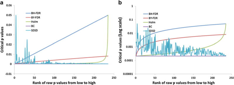
a Graphical representation of critical p values as a function of p value rank order. The standard BC is depicted as a constant line (purple) whose critical p value is independent of p value rank. The BH-FDR and BY-FDR results are depicted in blue and red, respectively. The Holm’s correction is shown in green. b Critical p values are plotted using a log scale to highlight differences among the various methods

Holm’s correction

The Holm’s procedure is a step down of the BC corresponding to a nonlinear inverse function where the independent variable is the p value rank order. Given the inverse function nature of the Holm’s correction formula, the Holm’s critical p value deviates negligibly from the BC critical p value until the p value rank-order approaches the total number of variables in the data set, after which the critical p value sharply approaches the significance level, α (Fig. 1). As a result, when the data set contains large numbers of variables, as in NMR data sets, the Holm’s correction is similar to the BC except for those variables whose p value rank-order approaches the total number of variables, N, in the data set. Variables with the lowest p value rank order, i.e., those variables with the smallest p values, are subjected the most stringent critical p value cutoff, whereas the variables with the largest p values are subjected to the most liberal critical p value cutoff, which rapidly approaches that of the raw significance level as the rank order approaches N.

Benjamini and Hochberg false discovery rate

The BH-FDR procedure [22] involves a linear step down from the significance level, α, to the BC critical p value. The step down factor is the rank order of the raw p value from low to high, i.e., the variable with the smallest p value will have the rank order value of 1 and the variable with the largest p value will have the rank order equal to N. The result is a linear extrapolation between the BC critical p value for the smallest raw p value to the significance level, α, for the largest raw p value (Fig. 1). A variable with a raw p value smaller than the BH-FDR-corrected critical p value is considered significant. The BH-FDR is naturally more sensitive than BC, however, as with the Holm’s correction, the smallest p value variables are subjected to the most stringent critical p value threshold. Furthermore, because the t test statistics are calculated based on the difference in group means divided by their pooled standard deviations [38], the t test statistic does not preserve or consider relative metabolite concentration information.

Benjamini–Yekutieli false discovery rate

The BY-FDR is essentially a scaled BH-FDR, where the scale factor is one over the accumulated sum of the p value rank orders. The result is a nearly linear function, like BH-FDR, that is scaled to a smaller maximum critical p value (Fig. 1). Consequently, BY-FDR is more stringent than BH-FDR for all variables, but more sensitive than BC. Again, BY-FDR has the characteristic, due to the multiplier being equal to the p value rank order, that the variable with the smallest p value has the most stringent critical p value and the variables with the largest p values have the most liberal critical p value threshold.

Standard deviation step down

In this manuscript, we introduce a new critical p value correction method, referred to as SDSD, with the goal of providing a technique that is appropriately less conservative than BC for analysis of partially dependent data sets, while at the same time, offering an approach that is fundamentally different from the preceding methods in that the variables with the smallest raw p values are not, by design, assigned the most stringent critical p value thresholds. SDSD achieves a fundamentally different critical p value profile by indirectly utilizing relative metabolite concentration, i.e., standard deviation, as its scale factor, instead of p value rank order. Analysis of the data set described below illustrates that there is no strict or ordered relationship between the raw variable p values and the critical p value, as is observed in the FDR and Holm’s procedures, where the smallest raw p value variables are ascribed the most stringent critical p values (Fig. 1). As a result, there is an increased probability that the smallest p value variables will be assigned more liberal critical p values, increasing their chance of being statistically significant, and potentially minimizing type II error rates. Metabolites with the greatest concentration in the sample are given higher priority, as long as their raw p values meet the significance level threshold. In doing so, the SDSD method places progressively more emphasis on the increasingly concentrated metabolites in the sample that experience statistically significant differences between comparison groups.

Comparison of statistical significance analysis of PCA loadings using BC, FDR, and SDSD

In the following sections, we examine NMR spectra of extracts of three different MCF-7 human breast cancer cell lines: one expressing the osteopontin-C splice variant (group C), one expressing the osteopontin-A splice variant (group A), and one transfected with an empty vector (group V) [25].

The PCA scores plot for the group C versus group V comparison using no scaling is shown in Fig. 2a. The groups separated into two statistically significant distinct clusters according to the Mahalanobis distance [39], D_M, and F test score (D_M=1.98 and F=5.32). Based on the most conservative BC method, three significant buckets were identified (red squares in Fig. 2b). The less conservative BH-FDR approach identified seven additional significant buckets for a total of ten (green triangles and black circles in Fig. 2b). SDSD also identified a total of ten buckets, including two significant buckets not found by either BC or BH-FDR. The two additional buckets had large loadings and therefore they are reasonable to be considered additional important buckets in the PCA. All buckets identified by BC were also significant by SDSD. However, two buckets identified as significant by BH-FDR were not significant by SDSD (black circles in Fig. 2b). The two insignificant buckets by BH-FDR had small loadings, and therefore it is unlikely that they should be considered important in the PCA.

Fig. 2.

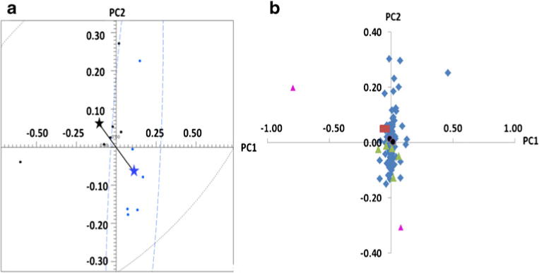
PCA analysis of the group C versus group V comparison. a PCA scores plot and b PCA loadings plot. Red squares are significant by all three methods: BC, FDR, and SDSD. Green triangles are significant by SDSD and FDR. Purple triangles are significant by SDSD but not by FDR. Black circles are significant by FDR but not by SDSD

The BY-FDR and Holm’s correction were also examined. To compare the PLS-DA loadings assessment, VIP was ana-lyzed as well (Table S2, Electronic supplementary material). From these investigations, we can see that Holm’s produced the same significant buckets as BC, as expected, while BY-FDR identified one more than BC but less than BH-FDR and SDSD. VIP (1 used as cut off) selected 77 variables with the largest p value=0.1, which is clearly too liberal. The main differences in the features of these methods are summarized in Table S1, Electronic supplementary material. For the following analysis, the BH-FDR was used as the representative FDR method for comparison with SDSD correction.

Figure 3 shows the distribution of bucket p values for the group C versus group V comparison with respect to standard deviation scaled to a maximum value of 1. Critical p value lines defined by significance level, BC, and SDSD are indicated in the plot. SDSD critical p values are represented by a curve as each bucket has a unique critical p value depending on its standard deviation rank order, as discussed above. Significant buckets based on the BC method, i.e., those having raw p values less than the BC critical value, are colored red. Orange solid circles indicate additional significant buckets identified by the SDSD correction method. The plot illustrates how, even though multiple buckets may have the same raw p value, only those that fall to the right of the SDSD critical p value line are considered statistically significant, which is a consequence of their being weighted by a higher standard deviation rank order.

Fig. 3.

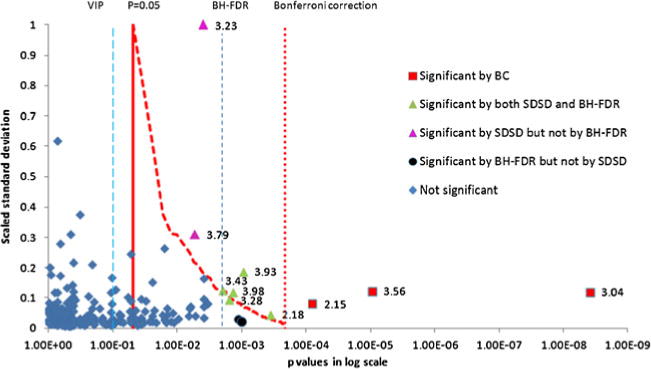
Distribution of raw bucket p values according to scaled standard deviation obtained from the C versus V comparison NMR data set. The solid red vertical line indicates the critical p value based on the significance level of α=0.05. The red dotted vertical line indicates the BC corrected critical p value. The red dashed curve shows SDSD critical values for peaks with raw p values between the significance level and the BC critical value. The y values for this curve are the normalized standard deviations for the bucket with its corresponding SDSD critical value. Red squares are significant by the BC method. Buckets with raw p values to the right of the SDSD critical values curve and to the left of the BC critical line (solid green triangles) indicate additional significant buckets identified by the SDSD method. Purple triangles are significant by SDSD but not by FDR. The resonance at 3.23 ppm belongs to O-phosphocholine and the resonance at 3.79 ppm belongs to glutamine. Black circles are significant by FDR but not by SDSD. The NMR pseudo spectra constructed from the PC1 loadings is shown in Fig. S4, Electronic supplementary material

Comparison of significance using SSA and PLS-DA

Figure 4a, b shows p values obtained from a Welch’s t test plotted against the absolute value of the first loading of PLS-DA for the group C versus group V comparison. An inverse relationship was observed as expected, i.e., buckets with the smallest raw p values typically corresponded to variables with the largest loadings. The log scale plot in Fig. 4b (and Fig. S2, Electronic Supplementary Material) clearly shows that p values are much more sensitive to variable differences compared to PLS-DA loadings in the very large difference regime (large loadings, small p values), where the p values span six orders of magnitude (10⁻³–10⁻⁹) over just a 13 % change in the magnitude of the largest PLS-DA loading (0.14–0.16). This observation is significant because the standard method of data presentation in the adjusted PLS-DA relies on heat-map color coding the PLS-DA spectrum by the absolute value of the loadings scaled to a maximum value of 1, but no SSA of the loadings is performed. As a result, there is increased possibility of false positive prediction if the p value of the largest loading happens to be relatively large.

Fig. 4.

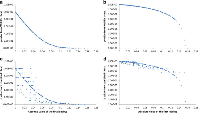
Scatter plot of p values from statistical significance analyses (group C versus group V) relative to the absolute value of the first PLS-DA loading. a Welch’s t test; b Welch’s t test with log y axis; c combined t test; d combined t test with log y axis. PLS-DA (R²X=0.759; Q²=0.554 from cross validation by SIMCA-P+ (v.11))

A similar trend was observed when a combined t test was applied in cases where one or more of the data sets failed to pass a normal data distribution test. In this case, a non-parametric Kruskal–Wallis test was used to determine the p value. In this application, the term combined t test refers to the fact that the technique used to determine the p values depended on whether or not the bucket data passed a Shapiro–Wilks normality test [40]. As a consequence, p values for some data were determined using a parametric Welch’s t test and some were determined using the non-parametric Kruskal–Wallis test [30], which is more accurate for small, non-normally distributed data sets. From Fig. 4c, d, an inverse relationship between p values and PLS-DA loadings was observed with the combined t test, however, the correlation between p value and loading magnitude was weaker, especially for small to mid-range loadings. The trend between p value and loading was stronger for the largest loadings, indicating that the SSA combined t test also offers some advantage compared with PLS-DA.

Comparison of important data features using BC, SDSD, and PLS-DA

PCA was conducted on another data set (group A versus group V) using no scaling preprocessing to illustrate the relative power of BC, SDSD, and PLS-DA. The resulting scores plot (Fig. 5a) indicated that the two groups separated into two statistically distinct clusters (Mahalanobis distance=5.36, F=38.8). SSA was calculated using both the Welch’s t test and the combined t test. Plots of the resulting p values versus PLS-DA loadings can be found in Fig. S3, Electronic supplementary material. A heat-map plot of the loadings based on the p values as a function of critical p value correction method is shown in Fig. 5b. Thirteen buckets were identified based on the BC threshold, whereas ten features were clearly identified from the PLS-DA plot (Fig. 5c). In the analysis of the PLS-DA plot, the bucket intensities in the “spectrum” are equal to the bucket loadings multiplied by the bucket standard deviations and the resulting peak is heat-map colored according to the scaled loading, where the largest loading is scaled to a value of 1. Therefore, in PLS-DA, the effective threshold refers to the smallest scaled loading for which a bucket is considered important; however, this does not directly indicate statistical significance. Whereas the BC is based on the assumption that all the variables are independent, we have already discussed above that this assumption cannot be justified in NMR spectra of human biofluids, and therefore, although the NMR spectra were represented by a total of 235 buckets, dividing the significance level of 0.05 by 235 to correct for multiple simultaneous testing will produce a too conservative critical p value threshold. Therefore, we plotted the most conservative SDSD result using 235 buckets, and then we softened the SDSD correction assuming just 100 independent variables. To accomplish, although the SDSD still had to be applied to 235 buckets, the step down factor was scaled to a value of 100/235=0.425 instead of 1.0 for each bucket. As a result, the critical p values for the conservative SDSD correction, i.e., SDSD (235), ranged from 0.05 (p_critical(1)=0.05/1=0.05) for the bucket with the largest standard deviation and lowest rank order to 0.0002 (p_critical(235)=0.05/235=0.0002) for the bucket with the smallest standard deviation and highest rank order assuming 235 independent variables with a step down factor of 1. For the less conservative SDSD correction, i.e., SDSD (100), the critical p values ranged from 0.05 (p_critical (1)=0.05/1=0.05) for the bucket with the largest standard deviation and lowest rank order to 0.0002 (p_critical (235)=0.05/(235*(100/235))=0.0005) for the bucket with the smallest standard deviation and highest rank order, assuming 100 independent variables with a step down factor of 100/235=0.425.

Fig. 5.

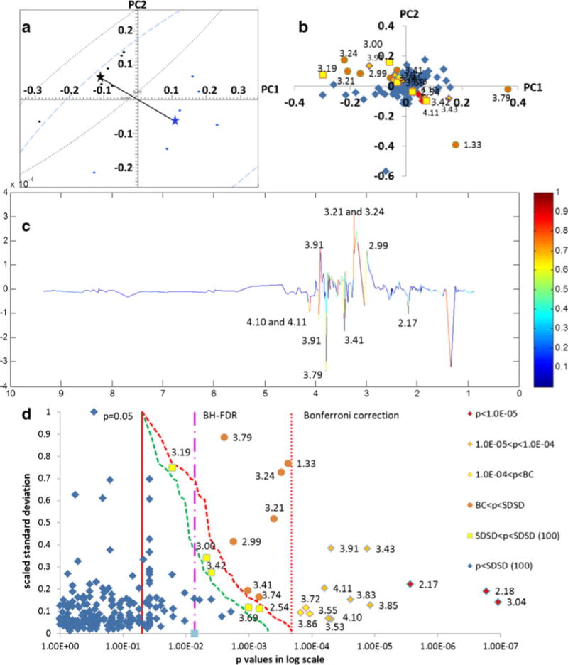
Comparison of group Aversus group V NMR-based metabonomics data using BC, SDSD, and PLS-DA. a PCA scores plot, b PCA loadings plot heat-map colored by bucket p values: red diamonds (p<10⁻⁵), orange diamonds (10⁻⁵<p<10⁻⁴), yellow diamonds (10⁻⁴<p<BC), orange circles (BC<p<SDSD correction (235 variables), and yellow squares (SDSD correction<p<SDSD (100 variables). c Loadings plot of the first latent variable from PLS-DA. d Buckets p value distribution according to scaled standard deviation. The colors and symbols of the markers are the same as in (a). The solid red vertical line indicates the critical p value base on the significance level; the dotted red vertical line indicates the BC critical p value; the dashed red line indicates the SDSD critical p value line using 235 variables; and the dashed green line indicates the SDSD critical p value line using 100 variables. The threshold for significant buckets identified by the FDR method is indicated by the pink dashed–dotted line; all buckets to the right of this critical line are significant by FDR. The NMR pseudo spectra for these data constructed from the PC1 loadings is shown in Fig. S5, Electronic supplementary material

The significant buckets identified by all four methods are indicated in Fig. 5d, which shows the distribution of bucket p value according to scaled standard deviation. Statistically significant buckets are indicated with the same symbols and coloring scheme as in Fig. 5b. The BC method identified 13 significant buckets, compared with 10 for the PLS-DA (Fig. 5c), whereas the SDSD (235) identified 7 additional buckets compared to BC for a total of 20, and the SDSD (100) identified 5 additional buckets compared with SDSD (235) for a total of 25. These results indicated that SDSD correction generates about twice as many significant buckets compared with PLS-DA, and SDSD is based on statistically relevant p values instead of scaled loadings. BH-FDR identified the most significant buckets, however, it is acknowledged in the literature to have the poorest control of family-wise error [41]. Indeed, the effective FDR critical value of 0.0073 corrects for only seven simultaneous tests compared with the most conservative BC, which corrected for 235. Hence, SDSD appears more realistic and reliable compared with FDR as a critical p value correction for multiple testing, while at the same time preserving and considering metabolite concentration information.

Conclusions

In this paper, we introduce the SDSD critical p value correction method. SDSD has several characteristics that are important relative to metabonomics investigations. First, SDSD offers increased sensitivity, i.e., power to detect true positives, in partially dependent data sets, while at the same time, attempting to maintain a constant family-wise type I error rate. In principle, SDSD can be quantitatively optimized utilizing a reasonable estimate of the number of dependent variables in a data set. Second, SDSD generates a fundamentally different profile of variable critical p values in which the smallest p value variables will not, by design, be assigned the most stringent critical p values, in contrast to the FDR and Holm’s methods, which ascribe the most stringent thresholds to the smallest p value variables. This characteristic should help minimize type II errors, i.e., false negatives. Third, SDSD indirectly utilizes metabolite concentration as its scale factor. The result is a progressively more sensitive critical p value for the most concentrated metabolites in solution. Ultimately, buckets with the smallest standard deviations, typically corresponding to the weakest concentration metabolites in solution, are subject to a critical p values approaching to the conservative BC value.

The rationale for SDSD is twofold. The first addresses the variable dependency in NMR data sets of human biological fluids. Application of the BC would require that all variables, i.e., NMR frequency buckets, are independent, which cannot be justified since several buckets can belong to the same metabolite, and many metabolites will be represented by multiple buckets. Said another way, many of the variables in a NMR data set will, in fact, be dependent. Therefore, the appropriate correction for multiple simultaneous testing will naturally be less stringent compared with the conservative BC method. The second is concerning the choice to place increasing emphasis on stronger features in the data set. In so doing, we skew the analysis so that the most liberal critical p values tend to be assigned to the most concentrated metabolites in the biofluid and the most stringent critical p values are ascribed to the most weakly concentrated metabolites in the same sample. While the assumption that changes in the most abundant metabolites in solution are more important than changes in the weakest represented metabolites in solution may not be universally true, SDSD provides a tool to filter or “skew” the analysis in such a way that focuses attention on the most concentrated metabolites in solution when such an approach is desirable or justified. An intriguing consequence of indirectly using metabolite concentration as the scale factor is that SDSD generates a fundamentally different profile of critical p values compared with existing FDR and Holm’s corrections, ascribing a more liberal critical p value cutoff to the lowest p value variables and potentially minimizing type II error rates, i.e., false negatives.

References

- 1.Lindon J, Nicholson J, Holmes E, Everett J. Metabonomics: metabolic processes studied by NMR spectroscopy of biofluids. Concepts Magn Reson. 2000;12(5):289–320. doi: 10.1002/1099-0534(2000)12:5<289::AID-CMR3>3.0.CO;2-W. [Google Scholar]
- 2.Lindon JC, Nicholson JK, Holmes E. The handbook of metabonomics and metabolomics. Elsevier; Amsterdam: 2007. [Google Scholar]
- 3.Beckonert O, Keun H, Ebbels T, Bundy J, Holmes E, Lindon J, Nicholson J. Metabolic profiling, metabolomic and metabonomic procedures for NMR spectroscopy of urine, plasma, serum and tissue extracts. Nat Protoc. 2007;2(11):2692–2703. doi: 10.1038/nprot.2007.376. [DOI] [PubMed] [Google Scholar]
- 4.Halouska S, Powers R. Negative impact of noise on the principal component analysis of NMR data. J Magn Reson. 2006;178(1):88–95. doi: 10.1016/j.jmr.2005.08.016. [DOI] [PubMed] [Google Scholar]
- 5.Choi Y, Kim H, Hazekamp A, Erkelens C, Lefeber A, Verpoorte R. Metabolomic differentiation of cannabis sativa cultivars using H-1 NMR spectroscopy and principal component analysis. J Nat Prod. 2004;67(6):953–957. doi: 10.1021/np049919c. [DOI] [PubMed] [Google Scholar]
- 6.Romick-Rosendale L, Goodpaster A, Hanwright P, Patel N, Wheeler E, Chona D, Kennedy M. NMR-based metabonomics analysis of mouse urine and fecal extracts following oral treatment with the broad-spectrum antibiotic enrofloxacin (Baytril) Magn Reson Chem. 2009;47:S36–S46. doi: 10.1002/mrc.2511. [DOI] [PubMed] [Google Scholar]
- 7.Wishart D. Quantitative metabolomics using NMR. Trac Trends Anal Chem. 2008;27(3):228–237. doi: 10.1016/j.trac.2007.12.001. [DOI] [Google Scholar]
- 8.Gu H, Pan Z, Xi B, Asiago V, Musselman B, Raftery D. Principal component directed partial least squares analysis for combining nuclear magnetic resonance and mass spectrometry data in metabolomics: application to the detection of breast cancer. Anal Chim Acta. 2011;686(1–2):57–63. doi: 10.1016/j.aca.2010.11.040. [DOI] [PMC free article] [PubMed] [Google Scholar]
- 9.Fonville J, Richards S, Barton R, Boulange C, Ebbels T, Nicholson J, Holmes E, Dumas M. The evolution of partial least squares models and related chemometric approaches in metabonomics and metabolic phenotyping. J Chemometr. 2010;24(11–12):636–649. doi: 10.1002/cem.1359. [DOI] [Google Scholar]
- 10.Trygg J, Holmes E, Lundstedt T. Chemometrics in meta-bonomics. J Proteome Res. 2007;6(2):469–479. doi: 10.1021/pr060594q. [DOI] [PubMed] [Google Scholar]
- 11.Van Den Berg R, Hoefsloot H, Westerhuis J, Smilde A, Van Der Werf M. Centering, scaling, and transformations: improving the biological information content of metabolomics data. Bmc Genomics. 2006;7 doi: 10.1186/1471-2164-7-142. [DOI] [PMC free article] [PubMed] [Google Scholar]
- 12.Cloarec O, Dumas M, Craig A, Barton R, Trygg J, Hudson J, Blancher C, Gauguier D, Lindon J, Holmes E, Nicholson J. Statistical total correlation spectroscopy: an exploratory approach for latent biomarker identification from metabolic H-1 NMR data sets. Anal Chem. 2005;77(5):1282–1289. doi: 10.1021/ac048630x. [DOI] [PubMed] [Google Scholar]
- 13.Wei S, Zhang J, Liu L, Ye T, Gowda G, Tayyari F, Raftery D. Ratio analysis nuclear magnetic resonance spectroscopy for selective metabolite identification in complex samples. Anal Chem. 2011;83(20):7616–7623. doi: 10.1021/ac201625f. [DOI] [PMC free article] [PubMed] [Google Scholar]
- 14.Cloarec O, Dumas M, Trygg J, Craig A, Barton R, Lindon J, Nicholson J, Holmes E. Evaluation of the orthogonal projection on latent structure model limitations caused by chemical shift variability and improved visualization of biomarker changes in H-1 NMR spectroscopic metabonomic studies. Anal Chem. 2005;77(2):517–526. doi: 10.1021/ac048803i. [DOI] [PubMed] [Google Scholar]
- 15.Claus S, Tsang T, Wang Y, Cloarec O, Skordi E, Martin F, Rezzi S, Ross A, Kochhar S, Holmes E, Nicholson J. Systemic multi-compartmental effects of the gut microbiome on mouse metabolic phenotypes. Molecular Systems Biology. 2008;4 doi: 10.1038/msb.2008.56. [DOI] [PMC free article] [PubMed] [Google Scholar]
- 16.Wang B, Goodpaster AM, Kennedy MA. Investigating the coefficient of variation, signal-to-noise ratio, and effects of normali-zation to aid in validation of biomarkers in NMR-based metabonomic studies. Chemometr Intell Lab Syst. 2013 doi: 10.1016/j.chemolab.2013.07.007. (in press) [DOI] [PMC free article] [PubMed] [Google Scholar]
- 17.Broadhurst DI, Kell DB. Statistical strategies for avoiding false discoveries in metabolomics and related experiments. Metabolomics. 2006;2(4):171–196. doi: 10.1007/s11306-006-0037-z. [DOI] [Google Scholar]
- 18.Reiner A, Yekutieli D, Benjamini Y. Identifying differentially expressed genes using false discovery rate controlling procedures. Bioinformatics. 2003;19(3):368–375. doi: 10.1093/bioinformatics/btf877. [DOI] [PubMed] [Google Scholar]
- 19.Narum S. Beyond Bonferroni: less conservative analyses for conservation genetics. Conserv Genet. 2006;7(5):783–787. doi: 10.1007/s10592-005-9056-y. [DOI] [Google Scholar]
- 20.Perneger T. What’s wrong with Bonferroni adjustments. Br Med J. 1998;316(7139):1236–1238. doi: 10.1136/bmj.316.7139.1236. [DOI] [PMC free article] [PubMed] [Google Scholar]
- 21.Nakagawa S. A farewell to Bonferroni: the problems of low statistical power and publication bias. Behav Ecol. 2004;15(6):1044–1045. doi: 10.1093/beheco/arh107. [DOI] [Google Scholar]
- 22.Benjamini Y, Hochberg Y. Controlling the false discovery rate—a practical and powerful approach to multiple testing. J R Stat Soc Ser B Methodol. 1995;57(1):289–300. [Google Scholar]
- 23.Benjamini Y, Yekutieli D. The control of the false discovery rate in multiple testing under dependency. Annal Stat. 2001;29(4):1165–1188. [Google Scholar]
- 24.Eriksson L, Johansson E, Kettaneh-Wold N, Trygg J, Wikström C, Wold S. Multi- and megavariate data analysis: part II: advanced applications and method extensions. Umetrics Inc. 2006 http://urn.kb.se/resolve?urn=urn:nbn:se:umu:diva-12897.
- 25.He B, Mirza M, Weber G. An osteopontin splice variant induces anchorage independence in human breast cancer cells. Oncogene. 2006;25(15):2192–2202. doi: 10.1038/sj.onc.1209248. [DOI] [PubMed] [Google Scholar]
- 26.Gottschalk M, Ivanova G, Collins D, Eustace A, O’connor R, Brougham D. Metabolomic studies of human lung carcinoma cell lines using in vitro H-1 NMR of whole cells and cellular extracts. NMR Biomed. 2008;21(8):809–819. doi: 10.1002/nbm.1258. [DOI] [PubMed] [Google Scholar]
- 27.Watanabe M, Sheriff S, Ramelot T, Kadeer N, Cho J, Lewis K, Balasubramaniam A, Kennedy M. NMR based metabonomics study of dag treatment in a c2c12 mouse skeletal muscle cell line myotube model of burn-injury. Int J Pept Res Ther. 2011;17(4):281–299. doi: 10.1007/s10989-011-9264-x. [DOI] [Google Scholar]
- 28.Zhang S, Zheng C, Lanza I, Nair K, Raftery D, Vitek O. Interdependence of signal processing and analysis of urine H-1 NMR spectra for metabolic profiling. Anal Chem. 2009;81(15):6080–6088. doi: 10.1021/ac900424c. [DOI] [PMC free article] [PubMed] [Google Scholar]
- 29.Lindon JC, Nicholson JK, Holmes E. The handbook of metabonomics. NMR spectroscopy techniques for application to metabonomics. Elsevier; Amsterdam: 2007. [Google Scholar]
- 30.Goodpaster A, Romick-Rosendale L, Kennedy M. Statistical significance analysis of nuclear magnetic resonance-based metabonomics data. Anal Biochem. 2010;401(1):134–143. doi: 10.1016/j.ab.2010.02.005. [DOI] [PubMed] [Google Scholar]
- 31.Eriksson L, Umetrics A. Multi- and megavariate data analysis. P. 1, basic principles and applications. Umetrics Academy; Umeå: 2006. [Google Scholar]
- 32.Nichols T, Hayasaka S. Controlling the familywise error rate in functional neuroimaging: a comparative review. Stat Methods Med Res. 2003;12(5):419–446. doi: 10.1191/0962280203sm341ra. [DOI] [PubMed] [Google Scholar]
- 33.Holm S. A simple sequentially rejective multiple test procedure. Scand J Stat. 1979;6(2):65–70. [Google Scholar]
- 34.Hochberg Y. A sharper bonferroni procedure for multiple tests of significance. Biometrika. 1988;75(4):800–802. doi: 10.1093/biomet/75.4.800. [DOI] [Google Scholar]
- 35.Beger R, Schnackenberg L, Holland R, Li D, Dragan Y. Metabonomic models of human pancreatic cancer using 1d proton NMR spectra of lipids in plasma. Metabolomics. 2006;2(3):125–134. doi: 10.1007/s11306-006-0026-2. [DOI] [Google Scholar]
- 36.Simes R. An improved bonferroni procedure for multiple tests of significance. Biometrika. 1986;73(3):751–754. doi: 10.1093/biomet/73.3.751. [DOI] [Google Scholar]
- 37.Holland B, Copenhaver M. Improved Bonferroni-type multiple testing procedures. Psychol Bull. 1988;104(1):145–149. doi: 10.1037//0033-2909.104.1.145. [DOI] [Google Scholar]
- 38.Ruxton G. The unequal variance t-test is an underused alternative to Student’s t-test and the Mann–Whitney u test. Behav Ecol. 2006;17(4):688–690. doi: 10.1093/beheco/ark016. [DOI] [Google Scholar]
- 39.Goodpaster A, Kennedy M. Quantification and statistical significance analysis of group separation in NMR-based metabonomics studies. Chemometr Intell Lab Syst. 2011;109(2):162–170. doi: 10.1016/j.chemolab.2011.08.009. [DOI] [PMC free article] [PubMed] [Google Scholar]
- 40.Shapiro S, Wilk M. An analysis of variance test for normality (complete samples) Biometrika. 1965;52:591. doi: 10.2307/2333709. [DOI] [Google Scholar]
- 41.Blaise B, Shintu L, Elena B, Emsley L, Dumas M, Toulhoat P. Statistical recoupling prior to significance testing in nuclear magnetic resonance based metabonomics. Anal Chem. 2009;81(15):6242–6251. doi: 10.1021/ac9007754. [DOI] [PubMed] [Google Scholar]
Associated Data
This section collects any data citations, data availability statements, or supplementary materials included in this article.