A Two-Sample Test for Equality of Means in High Dimension

Abstract

We develop a test statistic for testing the equality of two population mean vectors in the “large-p-small-n” setting. Such a test must surmount the rank-deficiency of the sample covariance matrix, which breaks down the classic Hotelling T² test. The proposed procedure, called the generalized component test, avoids full estimation of the covariance matrix by assuming that the p components admit a logical ordering such that the dependence between components is related to their displacement. The test is shown to be competitive with other recently developed methods under ARMA and long-range dependence structures and to achieve superior power for heavy-tailed data. The test does not assume equality of covariance matrices between the two populations, is robust to heteroscedasticity in the component variances, and requires very little computation time, which allows its use in settings with very large p. An analysis of mitochondrial calcium concentration in mouse cardiac muscles over time and of copy number variations in a glioblastoma multiforme data set from The Cancer Genome Atlas are carried out to illustrate the test.

1 Introduction

In many applications it is desirable to test whether the means of high-dimensional random vectors are the same in two populations. Often, the number of components in the random vectors exceeds the number of sampled observations, the so-called “large-p-small-n” problem, and conventional test statistics become unviable. Given the steadily growing availability and interest in high-dimensional data, particularly in biological applications, test statistics that are viable for high-dimensional data are in increasing demand. The challenge when p > > n is to model the structure of dependence among the p components without estimating each of the p(p + 1)/2 unique entries in the full covariance matrix. The classical test for equal mean vectors between two populations is Hotelling’s T² test, but the test statistic is undefined when p is larger than the sum of the sample sizes (minus 2), because it involves inverting the p × p sample covariance matrix. Several procedures are available which circumvent full covariance matrix estimation. We acheive this in the important case in which the p components admit an ordering in time, space, or in another index, such that the dependence between two components is related to their displacement. When measurements are taken along a chromosome, for example, the location of each measurement is recorded, providing an index over which dependence may be modeled, affording gains in power. For concreteness, it is here assumed that the components admit a unidirectional ordering.

To fix notation, let X₁, X₂, . . ., $X_n\in {\mathbb{R}}^p$ and Y₁, Y₂, . . ., $Y_m\in {\mathbb{R}}^p$ be independent identically distributed random samples from two populations having p × 1 mean vectors μ₁ and μ₂ and p × p covariance matrices Σ₁ and Σ₂, respectively. The hypotheses of interest become H₀ : μ₁ = μ₂ versus H₁ : μ₁ ≠ μ₂.

There are some methods available for testing H₀ : μ₁ = μ₂ versus H₁ : μ₁ ≠ μ₂ in the “large-p-small-n” setting. Srivastava (2007) presented a modification of Hotelling’s T² statistic which handles the singularity of the sample covariance matrix by replacing its inverse with the Moore-Penrose inverse. Wu et al. (2006) proposed the pooled component test, for which the test statistic is the sum of the squared univariate pooled two-sample t-statistics for all p vector components, which they assumed to follow a scaled chi-square distribution. Bai & Saranadasa (1996) presented a test statistic which uses only the trace of the sample covariance matrix and performs well when the random vectors of each population can be expressed as linear transformations of zero-mean i.i.d. random vectors with identity covariance matrices. Each of these methods assumes a common covariance matrix between the two populations, that is that Σ₁ = Σ₂.

More recently, under a setup similar to that of Bai & Saranadasa (1996), but which accommodates unequal covariances, Chen & Qin (2010) introduced a method (hereafter called the Ch-Q test), which allows Σ₁ ≠ Σ₂ and sidesteps covariance matrix estimation altogether. Srivastava & Kubokawa (2013) proposed a method (hereafter called the SK test) for multivariate analysis of variance in the large-p-small-n setting, of which the high-dimensional two-sample problem is an instance. Cai et al. (2014) presented a test (hereafter called the CLX test) based upon the supremum of standardized differences between the observed mean vectors, and offer an illuminating discussion about the conditions under which supremum-based tests are likely to outperform sum-of-squares-based tests, which include the Ch-Q and SK tests as well as the test we introduce in this paper. If the differences between μ₁ and μ₂ are rare, but large where they occur, i.e. the signals are sparse but strong, a supremum-based test should have greater power than a sum-of-squares-based test. The reason is that tests which sum the differences across a large number of indices will not be greatly influenced by a very small number of large differences. If, however, there are many differences between μ₁ and μ₂, but these differences are small, i.e. the signals are dense but weak, the supremum of the differences across all the indices will not likely be extreme enough to arouse suspicion of the null. A sum-of-squares based test statistic, however, will represent an accumulation of the large number of weak signals, and will have more power. Dense-but-weak signal settings do exist, for example in the analysis of copy number variations, where mildly elevated or reduced numbers of DNA segment copies in cancer patients are believed to occur over regions of the chromosome rather than at isolated points (Olshen et al. (2004), Baladandayuthapani et al. (2010)). It is for such cases that our test is designed.

Section 2 describes the GCT test statistic and Section 3 gives its asymptotic distribution. Section 4 presents a simulation study of the GCT, comparing its performance with that of the Ch-Q, SK, and CLX tests in terms of power and maintenance of nominal size. Section 5 implements the GCT as well as the Ch-Q, SK, and CLX tests on a copy number data set and a time series data set. Concluding remarks appear in Section 7 and the Appendix provides proofs of the main results. Full details for the proofs may be found in the Supplementary Material.

2 Test Statistic

The GCT statistic is computed as follows. Let $T_n=p^{-1}(t_{n1}^2+t_{n2}^2+\cdots +t_{np}^2)$, where

$$t_{nj}^2={({\overline{X}}_{nj}-{\overline{Y}}_{mj})}^2{(s_{nj}^2∕n+{\vartheta }_{mj}^2∕m)}^{-1}$$ (1)

for j = 1, . . ., p, where X̄_nj and Ȳ_mj are the sample means of the j^th vector component and $s_{nj}^2$ and ${\vartheta }_{mj}^2$ are the sample variances of the j^th vector component for the X and Y samples, respectively. Thus T_n is the mean of the squared unpooled univariate two-sample t-statistics $t_{nj}^2$ over all components j = 1, . . ., p.

The GCT statistic is a centered and scaled version of T_n defined as $G_n\equiv p^{1∕2}(T_n-{\widehat{\xi }}_n)∕{\widehat{\zeta }}_n$, where ${\widehat{\xi }}_n$ and $p^{1∕2}∕{\widehat{\zeta }}_n$ are described below. The equal means hypothesis is rejected at level α when |G_n|> Φ^–1(1 – α/2), where Φ(·) is the standard normal cumulative distribution function.

In what shall be called the moderate-p version of the test, ${\widehat{\xi }}_n\equiv 1$, so that $G_n^{\left(M\right)}\equiv p^{1∕2}(T_n-1)∕{\widehat{\zeta }}_n$. For the large-p version, higher-order expansions suggest a centering of the form ${\widehat{\xi }}_n\equiv 1+n^{-1}{\widehat{a}}_n+n^{-2}{\widehat{b}}_n$, so that

$$G_n^{\left(L\right)}\equiv p^{1∕2}\{T_n-(1+n^{-1}{\widehat{a}}_n+n^{-2}{\widehat{b}}_n)\}∕{\widehat{\zeta }}_n.$$ (2)

The quantities ${\widehat{a}}_n$ and ${\widehat{b}}_n$ are defined as ${\widehat{a}}_n\equiv ({\widehat{c}}_{n1}+\cdots +{\widehat{c}}_{np})∕p$ and ${\widehat{b}}_n\equiv ({\widehat{d}}_{n1}+\cdots +{\widehat{d}}_{np})∕p$, where ${\widehat{c}}_{nj}$ and ${\widehat{d}}_{nj}$ are obtained by plugging sample moments into the expressions given in Lemma 1 for c_nj and d_nj for each of the components j = 1, . . ., p.

Though T_n is a mean of squared marginal two-sample t-statistics, the construction of the scaling will account for the dependence among them. In both the moderate- and large-p versions of the test statistic, the scaling $p^{1∕2}∕{\widehat{\zeta }}_n$ is the same. Let

$$\widehat{\gamma }\left(k\right)={(p-k)}^{-1}\sum _{j=1}^{p-k}(t_{nj}^2-T_n)(t_{n(j+k)}^2-T_n),$$ (3)

which is the sample autocovariance function of the squared t-statistics. Then the scaling ${\widehat{\zeta }}_n$ is defined such that

$${\widehat{\zeta }}_n^2\equiv \sum _{\mid k\mid <L}w(k∕L)\widehat{\gamma }\left(k\right),$$ (4)

where w(x) is an even, piecewise function of x such that w(0) = 1, |w(x)|≤ 1 for all x, and w(x) = 0 for |x|> 1, and L is a user-selected lag window size.

The choices of the lag window w(·) considered here are the Parzen window

$$w_p\left(x\right)=\{\begin{array}{cc}1-6{\mid x\mid }^2+6{\mid x\mid }^3,\hfill & \mid x\mid <1∕2\hfill \\ 2{(1-\mid x\mid )}^3.\hfill & 1∕2\le x\le 1\hfill \\ 0,\hfill & \mid x\mid >1\hfill \end{array}\phantom{\}}$$

found in Brockwell & Davis (2009) and the trapezoid window

$$w_T(k∕r)=\{\begin{array}{cc}1,\hfill & \mid k\mid <[L∕2]\hfill \\ 1-\left(\frac{k-[L∕2]}{r-[L∕2]}\right),\hfill & [L∕2]\le k\le L\hfill \\ 0,\hfill & \mid k\mid >L\hfill \end{array}\phantom{\}}$$

from Politis & Romano (1995), where [x] denotes the largest integer not exceeding x.

3 Main Results

Let $\alpha \left(r\right)=\sup \{\alpha ({\mathcal{F}}_1^k,{\mathcal{F}}_{k+r}^p):1\le k\le p-r\}$, where ${\mathcal{F}}_a^b\equiv {\mathcal{F}}_{a,n}^b=\sigma \langle \{t_{nj}:a\le j\le b\}\rangle$ and where for any σ-fields, $\mathcal{F}$ and $\mathcal{G}$,

$$\alpha (\mathcal{F},\mathcal{G})=\sup \{\mid P(A\cap B)-P\left(A\right)P\left(B\right)\mid :A\in \mathcal{F},B\in \mathcal{G}\}$$

denotes the strong mixing coefficient between $\mathcal{F}$ and $\mathcal{G}$. Then the following conditions are assumed in deriving the asymptotic distribution of the test statistic T_n.

• (C.1) For some δ ∈ (0, ∞), (i) ${\sum }_{r=1}^{\infty }\alpha {\left(r\right)}^{\delta ∕(2+\delta )}<\infty$, and (ii) $E{\mid t_{nj}^2\mid }^{2r+\delta }<c<\infty$ for all j = 1, . . ., p for some integer r ≥ 1.

• (C.2) The limit ${\lim }_{n\to \infty }\frac{1}{p-k}{\sum }_{j=1}^{p-k}\mathrm{Cov}(t_{nj}^2,t_{n(j+k)}^2)=\gamma \left(k\right)$ exists for all k > 0.

• (C.3)

  1. max{E|X_1j|¹⁶, E|Y_1j|¹⁶, j = 1, . . ., p} = O(1).
  2. min{Var(X_1j), Var(Y_1j)} > c > 0.

The following theorem establishes the asymptotic normality of the test statistic under the appropriate centering and scaling.

Theorem 1 Suppose that p ≡ p_n = o(n⁶) and (C.1)–(C.3) hold with r = 1 in (C.1). Then

$$\underset{x\in \mathbb{R}}{\sup }\mid P(T_n-1<x)-\Phi \{\sqrt{p}(x-n^{-1}{a}_n-n^{-2}{b}_n)∕{\tau }_{\infty }\}\mid =o\left(1\right),$$

where ${\tau }_{\infty }^2=\gamma \left(0\right)+2{\sum }_{k=1}^{\infty }\gamma \left(k\right)$ and a_n = (c_n1 + ··· + c_np)/p and b_n = (d_n1 + ··· + d_np)/p, where c_nj and d_nj for j = 1, . . ., p are as in Lemma 1 in the Appendix.

Remark 1 Theorem 1 shows that $G_n\equiv p^{1∕2}(T_n-{\widehat{\xi }}_n)∕{\widehat{\zeta }}_n{\to }^d$ Normal(0, 1) as n → ∞.

3.1 Technical Details

The choice of the centering quantity ${\widehat{\xi }}_n$ comes from noting that ET_n = 1+O(n^–1) as n → ∞. This follows from the fact that t_nj converges in distribution to Z, where Z ~ Normal(0, 1), for all j = 1, . . ., p, and EZ² = 1. Thus $E\left\{\sqrt{p}(T_n-1)\right\}=\sqrt{p}O\left(n^{-1}\right)$, so that when ${\widehat{\xi }}_n\equiv 1$, the expectation of the test statistic differs from zero by $\sqrt{p}O\left(n^{-1}\right)$, restricting p to grow at a rate such that p = o(n²). When ${\widehat{\xi }}_n\equiv 1+n^{-1}{\widehat{a}}_n+n^{-2}{\widehat{b}}_n$, the expectation of the test statistic is $\sqrt{p}O\left(n^{-3}\right)$, allowing p = o(n⁶). Hence the “moderate-” and “large-p” designations. One may also consider an intermediate-p version of the test which uses only $n^{-1}{\widehat{a}}_n$ in the centering correction, allowing p = o(n⁴), but its performance is not investigated here.

While the large-p test allows for p = o(n⁶), an advantage of the moderate-p test is its robustness to outliers. The centering correction in the large-p test involves high-order sample moments which are volatile when the data come from a very heavy-tailed distribution, in which case the centering value of 1 is preferable.

The formulation of ${\widehat{\zeta }}_n$ rests on the assumption that the p components admit a logical ordering such that their dependence is autocovarying and diminishing as components are further removed—that is, that the covariance between components may be described with an autocovariance function that decays sufficiently fast. In the proof of Theorem 1, the asymptotic variance of p^1/2T_n under some regularity conditions is shown to be ${\sum }_{h=-\infty }^{\infty }\gamma \left(h\right)$, which is equal to 2π times the spectral density f(·) of the sequence ($t_{n1}^2,t_{n2}^2,\dots$) evaluated at 0. Thus $\widehat{f}\left(0\right)={\left(2\pi \right)}^{-1}{\sum }_{\mid k\mid <L}w(k∕L)\widehat{\gamma }\left(k\right)$ provides the scaling in (4).

3.2 Power of the Generalized Component Test

In order to compute the asymptotic power of the GCT, the expected value of $T_n=p^{-1}(t_{n1}^2,\dots ,t_{np}^2)$ must be computed under the alternative H₁ : μ_1j – μ_2j = δ_j for j = 1, . . ., p where δ_j ≠ 0 for at least one j. Let ${\xi }_n^{\left(1\right)}$ denote E(T_n|H₁ true). Then the power of the GCT, which is $P(\mid p^{1∕2}(T_n-{\widehat{\xi }}_n)∕{\widehat{\zeta }}_n)\mid >z_{\alpha ∕2}\mid H_1\text{true})$, is equal to

$$1-P(-z_{\alpha ∕2}-p^{1∕2}({\xi }_n^{\left(1\right)}-{\widehat{\xi }}_n)∕{\widehat{\zeta }}_n<p^{1∕2}(T_n-{\xi }_n^{\left(1\right)}∕{\widehat{\zeta }}_n)<z_{\alpha ∕2}-p^{1∕2}({\xi }_n^{\left(1\right)}-{\widehat{\xi }}_n)∕{\widehat{\zeta }}_n\mid H_1\text{true}).$$

Under conditions (C.1)–(C.3) we can invoke the asymptotic normality of $p^{1∕2}(T_n-{\xi }_n^{\left(1\right)})∕{\widehat{\zeta }}_n$ and the consistency of ${\widehat{\zeta }}_n$ for ζ and approximate the power with

$$1-\{\Phi (z_{\alpha ∕2}-p^{1∕2}({\xi }_n^{\left(1\right)}-{\widehat{\xi }}_n)∕\zeta )-\Phi (-z_{\alpha ∕2}-p^{1∕2}({\xi }_n^{\left(1\right)}-{\widehat{\xi }}_n)∕\zeta )\}$$

so that it is a function of $p^{1∕2}({\xi }_n^{\left(1\right)}-{\widehat{\xi }}_n)∕\zeta$.

Given the tedium of computing ${\xi }_n^{\left(1\right)}=E\{p^{-1}{\sum }_{j=1}^p{t}_{nj}^2\mid H_1\text{true}\}-n{p}^{-1}{\sum }_{j=1}^{p}E[{({\overline{X}}_{nj}-{\overline{Y}}_{mj})}^2∕\{s_{nj}^2+(n∕m){\vartheta }_{mj}^2\}\mid H_1\text{true}]$ to within O(n^–3) of its true value as was done for ${\widehat{\xi }}_n$ under the null hypothesis (cf. Lemma 1), we replace $s_{nj}^2$ and ${\vartheta }_{mj}^2$ with their population values ${\sigma }_{1j}^2$ and ${\sigma }_{2j}^2$ and ${\xi }_n^{\left(1\right)}\approx 1+n{({\mu }_{1j}-{\mu }_{2j})}^2∕\{{\sigma }_{1j}^2+(n∕m){\sigma }_{2j}^2\}$.

If we may replace n, $p^{1∕2}({\xi }_n^{\left(1\right)}-{\widehat{\xi }}_n)∕\zeta$ with $n{p}^{-1∕2}{\sum }_{j=1}^p{\delta }_j^2∕\{{\sigma }_{1j}^2+(n∕m){\sigma }_{2j}^2\}∕\zeta$, then the power may be expressed

$$1-(\Phi [z_{\alpha ∕2}-n{p}^{-1∕2}\sum _{j=1}^p{\delta }_j^2∕\{{\sigma }_{1j}^2+(n∕m){\sigma }_{2j}^2\}∕\zeta ]-\Phi [-z_{\alpha ∕2}-n{p}^{-1∕2}\sum _{j=1}^p{\delta }_j^2∕\{{\sigma }_{1j}^2+(n∕m){\sigma }_{2j}^2\}∕\zeta ]).$$

From this expression we note that under p = o(n²)

$$\text{Power}\to \{\begin{array}{cc}1,\hfill & p^{1∕2}{n}^{-1}=o(\sum _{j=1}^p{\delta }_j^2∕\{{\sigma }_{1j}^2+(n∕m){\sigma }_{2j}^2\})\hfill \\ \alpha ,\hfill & \sum _{j=1}^p{\delta }_j^2∕\{{\sigma }_{1j}^2+(n∕m){\sigma }_{2j}^2\})=o\left(p^{1∕2}{n}^{-1}\right)\hfill \end{array}\phantom{\}}$$

For example, if δ_j = δp^–1/2 for j = 1, . . ., p for some δ > 0 then the power will converge to 1, but if δ_j = δp^–(1/2+ε) for j = 1, . . ., p the test will have “nonpower” above the significance level as n, p → ∞.

4 Simulation Studies

The performances of the GCT, Ch-Q, SK, and CLX tests were compared in terms of size control and power under various settings. For the sample sizes (n, m) = {(45, 60), (90, 120)} with p = 300, two-sample data were generated such that for each subject the p components were (i) independent (IND), (ii) ARMA dependent, or (iii) long-range (LR) dependent. For each dependence structure, the innovations used to generate each subject series were (a) Normal(0,1), (b) skewed innovations, coming from a gamma(4, 2) distribution centered at zero, thus having mean zero and variance 4(2)² = 16, and (c) heavy-tailed innovations from a Pareto(a, b) distibution with distribution function F(x) = 1 – (1 + x/b)^–1/a where the density was shifted to the origin and reflected across the vertical axis to form a “double” Pareto distribution. Under this double Pareto distribution,

$$E{\mid X\mid }^r=\{\begin{array}{cc}\infty ,\hfill & r\ge a\hfill \\ b^r\Gamma (a-r)\Gamma (1+r)∕\Gamma \left(a\right),\hfill & r<a.\hfill \end{array}\phantom{\}}$$

Once a zero-mean series was generated for each subject, it was added to the p × 1 mean vector μ₁ or μ₂, depending on the population to which the subject belonged. Under IND, the zero-mean series consisted of p independent identically distributed innovations from the chosen innovation distribution. For the ARMA dependence structure, p-length series from an ARMA process with AR parameters ϕ₁ = {0.4, –0.1} and MA parameters θ₁ = {0.2, 0.3} were used for both populations. Under the LR structure, realizations of zero-mean, long-range-dependent processes with self-similarity parameter H₁ = (1/2)(2 – 0.75) = 0.625 were used. The algorithm used for generating vectors of long-range dependent random variables is found in Hall et al. (1998).

At each sample size, dependence structure, and innovation distribution combination, a simulation was run in which Σ₁ = Σ₂ and in which Σ₂ = 2Σ₁, where the unequal covariance setting was imposed by scaling the zero-mean series for the population 2 subjects by √2.

For the CLX test, which features an equal-covariances and an unequal-covariances version, Cai et al. (2014) suggest first testing H₀ : Σ₁ = Σ₂ using a test from Cai et al. (2013) and then choosing the version of the CLX test accordingly. Since in practice it is generally not known whether Σ₁ = Σ₂ holds, the test of H₀ : Σ₁ = Σ₂ was performed in each simulation run to determine which version of the CLX test would be used. The CLX test requires an estimate for the precision matrix $\Omega ={\Sigma }_1^{-1}(={\Sigma }_2^{-1})$ or Ω = {Σ₁ + (n/m)Σ₂}^–1 for the unequal-covariances version. Of the two methods the authors suggest for estimating , that which is presented in Cai et al. (2011) and provided in the R package fastclime (Pang et al. (2013)) was chosen and implemented under default settings.

For power simulations, the alternate hypotheses were that μ₁ = 0 and ${\mu }_2={[\delta 1_{\beta p}^{\prime },\left(0\right)1_{(1-\beta )p}^{\prime }]}^{\prime }$, where 1_k was a k × 1 vector of ones, p was the number of components, and β ∈ [0, 1] was the proportion of the p components for which the difference in means was nonzero. The number of components p was fixed at 300 and the power was simulated for β ∈ {0, 0.1, 0.2, 0.4, 0.6, 0.8, 0.9, 1}. The difference or signal δ was chosen such that the signal to noise ratio δ/σ was equal to 1/8, where σ was the standard deviation of the innovations used to construct each series (each p-variate observation); thus δ = σ/8 was used.

Full factorial simulation results for {(45, 60), (90, 120)} × {IND, ARMA, LR} × {Normal, Skewed, Heavy-tailed} × {Σ₁ = Σ₂, Σ₂ = 2Σ₁} are given in the Supplementary Material and selected results are highlighted here. In addition to the factorial simulation, the tests were evaluated under heteroscedastic component variances and ultra-heavy tailed (infinite-variance) innovations.

4.1 Performance under normality

Table 1 displays the simulated Type I error rates of the four tests under the sample sizes (n, m) = (45, 60), (90, 120) across the three dependence structures under Normal(0, 1) innovations and for Σ₁ = Σ₂. For the GCT, results are given for the Parzen and trapezoid lag windows at lag window sizes L = 10, 15, 20 for the moderate-p (upper panel) and the large-p (lower panel) choice of the centering. The Ch-Q, SK, and CLX Type I error rates are duplicated in the upper and lower panels as the moderate- and large-p versions of the GCT were applied to the same 500 simulated data sets.

Table 1.

Type I error rates over S = 500 simulations with nominal size α = .05 for the moderate- and large-p GCT under the Parzen and trapezoid lag windows at lengths L = 10, 15, 20 and for the Ch-Q, SK, CLX tests under Normal(0, 1) innovations with Σ₁ = Σ₂.

p = 300, Σ1 = Σ2						Normal(0, 1) Innovations
${\widehat{\xi }}_n\equiv 1$						Parzen Window			Trapezoid Window
n	m	Cov	Ch-Q	SK	CLX	L = 10	L = 15	L = 20	L = 10	L = 15	L = 20
45	60	IND	0.07	0.04	0.09	0.06	0.07	0.07	0.06	0.08	0.07
		ARMA	0.06	0.04	0.08	0.06	0.07	0.07	0.07	0.08	0.07
		LR	0.05	0.04	0.10	0.06	0.06	0.07	0.08	0.09	0.07
90	120	IND	0.05	0.04	0.07	0.06	0.06	0.06	0.07	0.08	0.06
		ARMA	0.05	0.04	0.06	0.07	0.07	0.08	0.08	0.09	0.08
		LR	0.03	0.03	0.07	0.05	0.05	0.07	0.06	0.08	0.07

${\widehat{\xi }}_n\equiv 1+a_n∕n+b_n∕n^2$						Parzen Window			Trapezoid Window
n	m	Cov	Ch-Q	SK	CLX	L = 10	L = 15	L = 20	L = 10	L = 15	L = 20
45	60	IND	0.07	0.04	0.09	0.07	0.07	0.07	0.07	0.08	0.07
		ARMA	0.06	0.04	0.08	0.07	0.07	0.07	0.07	0.08	0.07
		LR	0.05	0.04	0.10	0.07	0.07	0.08	0.08	0.09	0.08
90	120	IND	0.05	0.04	0.07	0.06	0.06	0.07	0.07	0.08	0.07
		ARMA	0.05	0.04	0.06	0.08	0.08	0.08	0.08	0.09	0.08
		LR	0.03	0.03	0.07	0.06	0.06	0.06	0.07	0.09	0.06

The Ch-Q and SK tests maintained very close-to-nominal Type I error rates. The CLX test exhibited slightly inflated Type I error rates under the IND and LR dependence structures for the smaller sample sizes (n, m) = (45, 60), but maintained close-to-nominal rates for (n, m) = (90, 120). For the GCT, the Parzen window appeared to control the Type I error rate slightly better than the trapezoid window, and the Type I error rates were similar for the three choices of the lag window size.

Power simulation results under normal innovations appear in Figure S.6 of the Supplementary Material.

4.2 Effect of skewness

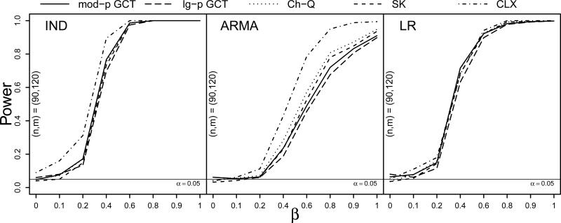
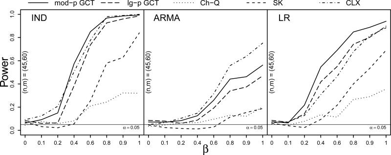
The results of the Type I error simulation with skewed innovations were similar to those in the Normal(0, 1) case and can be seen in Table S.3 of the Supplementary Material. For the power simulation, Figure 1 plots the proportion of rejections across 500 simulation runs against the proportion β of the p = 300 components in which μ₁ and μ₂ differed, where β ∈ {0, 0.1, 0.2, 0.4, 0.6, 0.8, 0.9, 1}. The three panels show the power curves of the four tests under the IND, ARMA, and LR dependence structures, respectively, when the innovations came from the centered gamma(4, 2) distribution and when the sample sizes were (n, m) = (90, 120). The four tests exhibited similar performance under these settings, though under independence the size of the CLX test was somewhat inflated, yet its power increased more rapidly in β than that of the other tests under ARMA dependence.

Figure 1.

Power curves at sample sizes (n, m) = (90, 120) for the moderate- and large-p GCT, Ch-Q, SK, and CLX tests against the proportion of nonzero mean differences β under IND, ARMA, and LR dependence (left to right) with centered gamma(4, 2) innovations and Σ₁ = Σ₂. Based on S = 500 simulations.

4.3 Effect of heavy-tailedness

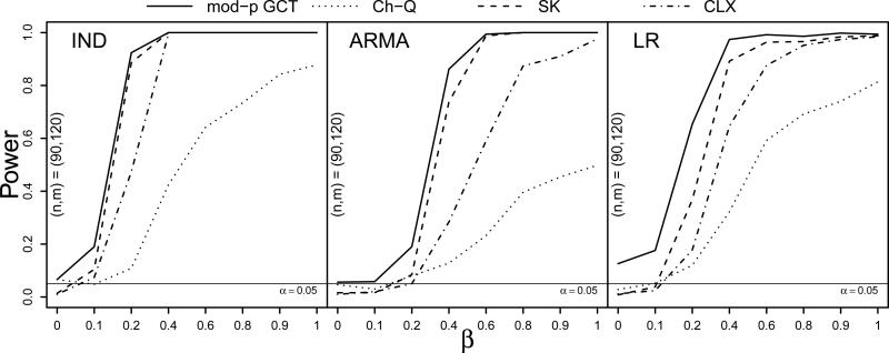
The results for the heavy-tailed simulation with innovations coming from the double Pareto(16.5, 8) distribution did not differ greatly from those of the normal- and skewed-innovations simulations. Full results may be found in the Supplementary Material. In order to assess the robustness of the GCT to violations of its moment conditions, ultra-heavy tailed data were simulated using innovations from a double Pareto(1.5, 1) distribution, which has infinite variance. Since the centering corrections ${\widehat{a}}_n$ and ${\widehat{b}}_n$ in the large-p GCT are computed using higher order sample moments, only the moderate-p GCT was here considered, as its centering of 1 gives it stability. Under these settings, the signal, which was set to δ = .5, is very weak relative to the noise, such that as the proportion β of non-null mean differences goes to 1, a dense-but-weak signal structure is simulated. The resulting power curves are shown in Figure 2, in which the Ch-Q test is seen to have much less power than the others; the CLX also suffers a reduction in power under ARMA and LR dependence. Under LR dependence, the size of the GCT was somwhat inflated, but it was very close to nominal for the IND and ARMA cases. In the ARMA case, the GCT exhibited greater power than the other tests across the range of alternatives.

Figure 2.

Power curves at sample sizes (n, m) = (90, 120) for the large-p GCT, Ch-Q, SK, and CLX tests against the proportion of nonzero mean differences β under IND, ARMA, and LR dependence (left to right) with double Pareto(1.5,1) innovations and Σ₁ = Σ₂. Based on S = 500 simulations.

4.4 Effect of heteroscedasticity

The effect of heteroscedasticity on the GCT may be anticipated by noting that $t_{nj}^2$ from (1) can be expressed

$$t_{nj}^2={\left[\frac{\sqrt{n}\{({\overline{X}}_{nj}-{\mu }_{1j})-({\overline{Y}}_{mj}-{\mu }_{2j})\}}{\sqrt{s_{nj}^2+(n∕m){\vartheta }_{mj}^2}}+\frac{\sqrt{n}{\delta }_j}{\sqrt{s_{nj}^2+(n∕m)}{\vartheta }_{mj}^2}\right]}^2$$ (5)

where δ_j = μ_1j – μ_2j, for j = 1, . . ., p. The second term is equal to zero under H₀. Under H₁, for a fixed difference δ_j, the variances ${\sigma }_{1j}^2$ and ${\sigma }_{2j}^2$ affect the magnitude of $t_{nj}^2$ such that very small values for ${\sigma }_{1j}^2$ and ${\sigma }_{2j}^2$ promote very large values of $t_{nj}^2$. Since th scaling ${\widehat{\zeta }}_n$ for T_n is a function of $\widehat{\gamma }(\cdot )$, the estimated autocovariance function of $t_{n1}^2$, $t_{n2}^2$, . . ., $t_{np}^2$, as seen from (3) and (4), extreme values of $t_{nj}^2$ will pull ${\widehat{\zeta }}_n$ upward, shrinking T_n toward zero. Extreme values of $t_{nj}^2$ will tend to occur if ${\sigma }_{1j}^2$ and ${\sigma }_{2j}^2$ are very small when δ_j ≠ 0. Although smaller variances ought to ensure a greater likelihood of rejecting H₀, if ${\widehat{\zeta }}_n$ is inflated by extreme values of $t_{nj}^2$, the GCT statistic will be close to zero, and the test will fail to reject, hence condition (C.3) (ii). Large values of ${\sigma }_{1j}^2$ and ${\sigma }_{2j}^2$ when δ_j = ≠ 0 will tend to reduce $t_{nj}^2$, but since it is bounded below by zero, extreme values will not occur. The size of the test should be robust to any scaling of the variances, as the second term in (5) will be zero when H₀ is true.

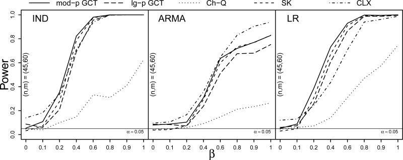
To investigate the impact of heterscedasticity on the performance of the four tests, the standard deviations of the components were each scaled by a realization from the exponential distribution with mean 1/2 shifted to the right by 1/2 such that the average scaling was 1 and so that the scaled variances were bounded away from 0. The power simulation with centered gamma(4, 2) innovations was repeated under these heteroscecastic conditions with (n, m) = (45, 60). Figure 3 exhibits a dramatic reduction in the power of the Ch-Q test due to heteroscedasticity. The CLX test exhibited somewhat inflated size under the IND and LR dependence structures, while the SK test and the GCT demonstrated robustness to the heteroscedstic variance scalings.

Figure 3.

Power curves at sample sizes (n, m) = (45, 60) for the moderate- and large-p GCT, Ch-Q, SK, and CLX tests against the proportion of nonzero mean differences β under IND, ARMA, and LR dependence (left to right) with heteroscedastic centered gamma(4, 2) innovations and Σ₁ = Σ₂. Based on S = 500 simulations.

4.5 Effect of unequal covariance matrices

Of the four tests, the SK test is the only one which assumes a common covariance matrix for the two populations. Cai et al. (2014) suggest first testing H₀ : Σ₁ = Σ₂ with a test from Cai et al. (2013) and implementing the equal or unequal covariances version of the CLX test accordingly. The Ch-Q and the GCT do not require any assumption or testing of equality between the covariance matrices. The SK is thus anticipated to perform more poorly than the others when the covariance matrices are unequal.

To impose inequality between Σ₁ and Σ₂, the zero-mean sequences for each subject from population two were scaled by √2 before the signal μ₂ was added. This imposed the condition that Σ₂ = 2Σ₁.

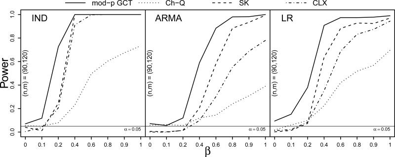
Figure 5 displays results for a simulation in which the variances of the second population were scaled by two and in which the variances in both populations were heteroscedastic. The SK lost much of its power under these settings, which was expected given its assumption of a common covariance matrix in the two populations. The Ch-Q test exhibited low power as before owing to the heteroscedasticity, but performed none the worse for the unequally scaled variances. The GCT achieved the greatest power under the LR dependence structure, having less power than the CLX test in the ARMA case.

Figure 5.

Power curves at sample sizes (n, m) = (90, 120) for the moderate-p GCT, Ch-Q, SK, and CLX tests against the proportion of nonzero mean differences β under IND, ARMA, and LR dependence (left to right) with double Pareto(1.5,1) innovations and Σ₂ = 2Σ₁. Based on S = 500 simulations.

Lastly, under the ultra heavy-tailed innovation distribution with unequally scaled covariances between the two populations, the GCT exhibited superior power to the Ch-Q, SK, and CLX tests under all three dependence stuctures at the (n, m) = (90, 120) sample sizes. Although the size of the GCT was somewhat inflated under the LR dependence structure, it maintained the nominal Type I error rate in the ARMA case, under which it achieved roughly 60% power when β = 0.4 while the CLX test achieved only about 10% power.

5 Copy Number Variation Example

The GCT, Ch-Q, SK, and CLX tests were each applied to a data set from The Cancer Genome Atlas containing copy number measurements at chromosomal copy number locations in 92 long-term-surviving patients, who survived for more than two years after their initial diagnosis and 138 short-term-surviving patients, who survived for fewer than 2 years after their initial diagnosis of a brain cancer called glioblastoma multiforme (GBM). Pinkel & Albertson (2005) suggest that the numbers of copies of certain DNA segments within a cell may be associated with cancer development and spread. It is thus of interest to identify regions along the genome in which high numbers of copies are associated with the incidence or severity of cancer, as such regions may harbor cancer-causing or tumor-suppressor genes. In studies having relatively few patients, several thousand copy number measurements are taken along each arm of each chromosome, which makes identifying regions for which two patient groups have different mean copy number profiles a high-dimensional problem. Additionally, it is believed that copy number variations between patient groups will occur over stretches of the chromosome (spanning multiple probes) rather than at isolated points (singleton probe locations) (Olshen et al. (2004), Baladandayuthapani et al. (2010)), suggesting a serial dependence over the chromosome as well as the presence of a dense-but-weak rather than a sparse-but-strong signal structure.

We restricted our analysis to the q arm of chromosome 1, the longest chromosome, on which there are 8,895 copy number measurements. Each measurement is a log-ratio of the number of copies at each location over 2, where 2 is the number of copies found in normal DNA. Positive measurements thus indicate duplications and negative measurements indicate deletions. The measurements, in conformity with the assumption of the GCT that the components of interest admit a logical ordering, are recorded along with their locations given in the number of base pairs from the end of the DNA strand. For many of the 8,895 components, there are a few missing values in either or both of the samples such that the average proportion of missing values per component is 0.0276 for the long-term survivors and 0.0273 for the short-term survivors. Prior to analysis, each missing value was replaced with the mean of the non-missing values for the same component in the same sample.

Although a test may reject H₀ : μ₁ = μ₂ when μ_j is the 8895 × 1 vector of copy number means for j = 1, 2, a wholesale conclusion for the entire arm of the chromosome is of little use if it is desired to identify particular regions in which copy number differences lie. In order to break the chromosome arm into meaningful regions in which the equal means hypothesis is of interest, we performed a method of segmentation called circular binary segmentation (CBS) from Olshen et al. (2004). This procedure locates change points in the copy number sequence for a single sequence of copy number values, and is implemented in the R package DNAcopy (Seshan & Olshen (2013)). In order to segment the q arm of chromosome 1 for equal means hypothesis testing when multiple patients are observed, the CBS procedure was applied to the 8895 × 1 vector of differences in means X̄ – Ȳ using weights equal to $s_j^2∕n+{\vartheta }_j^2∕m$ for j = 1, . . ., 8895. Before computing X̄, Ȳ, and $s_j^2$ and ${\vartheta }_j^2$ for j = 1, . . ., p, each series was smoothed using the function smooth.CNA() from the DNAcopy package. The CBS procedure provided 26 segments of varying lengths at the edges of which change points were detected in the vector of differences in means. As a set of 7 contiguous segments contained small numbers of markers (44, 14, 26, 39, 26, 21, 27) they were collapsed into a single segment having 197 markers, which left 20 regions within which the number of probes p ranged from 73 to 1811. Such splitting of the chromosome into windows or segments has been widely used in genome-wide association studies in searching for chromosomal regions in which genetic variants are associated with a continuous or dichotomous clinical outcome, as in Wu et al. (2011).

The large- and moderate-p GCT with lag window size L = (2/3)p^1/2 and the Ch-Q, SK, and CLX tests were applied to each of the twenty segments identified by the CBS procedure to test H_0k : μ_1k = μ_2k for k = 1, . . ., 20 (Though smoothing was used in identifying the segments, the analysis was carried out on the raw, unsmoothed data). Since the equal-means hypothesis was tested for twenty different regions simultaneously, the sets of p-values which each of the four tests generated were compared with the Benjamini & Hochberg (1995) discovery rate (FDR) threshold. For m tests of hypotheses, the m p-values are ordered p₍₁₎ ≤ p₍₂₎ ≤ . . . ≤ p_(m) and then the hypothesis to which p_(i) corresponds is rejected if i ≤ k, where k = max{j : p_(j) ≤ (j/m)q}. This procedure was originally shown to control the FDR at q for m independent hypothesis tests, though Benjamini & Yekutieli (2001) showed that for many common types of positive dependence among the m test statistics, the same procedure still adequately controls the FDR. The procedure was therefore applied to the twenty p-values computed from each test.

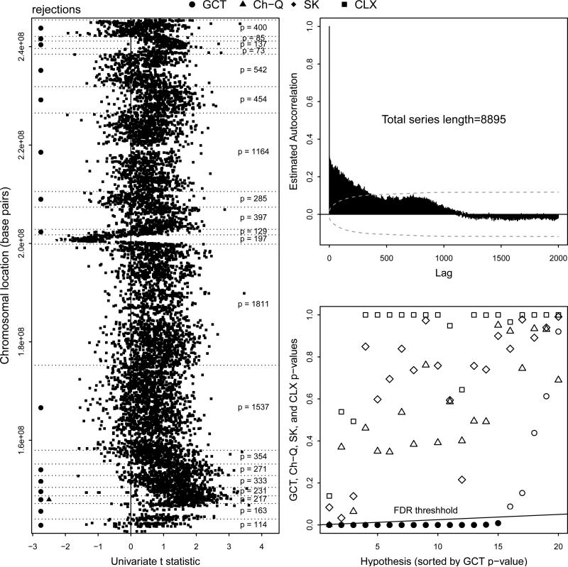
Figure 6 summarizes the analysis. The left panel displays the univariate two-sample t-statistics, which are the t_nj values for j = 1, . . ., 8895, against their locations in base pairs along the q arm of chromosome 1. The vertical line at zero marks the value around which the t-statistics would be centered under the null hypotheses, and the horizontal dotted lines delineate the CBS-selected segments of the chromosome arm. The numbers of copy number markers p within each segment appear on the right. Rejections acheived by the tests are marked with symbols appearing on the left, where rejections for each test are determined by the Benjamini & Hochberg (1995) FDR procedure.

Figure 6.

(Left) Univariate t-statistics (t_nj) plotted against base-pair location on q arm of chromosome 1. Filled symbols denote rejections from FDR procedure for the GCT, Ch-Q, SK, and CLX tests. The number of components p within each CBS-selected chromosomal region is shown. (Upper right) Estimated autocorrelation function for squared univariate t-statistics along q arm of chromosome 1 with large-lag confidence bands. (Lower right) FDR results, hypotheses sorted by GCT p-values. FDR rejection threshold shown with filled symbols denoting rejections.

The upper right panel of Figure 6 displays the estimated autocorrelation function of the squared two-sample univariate t-statistics, the $t_{nj}^2$ values for j = 1, . . ., 8895, along the q arm of chromosome 1. The 95% confidence bounds using the large-lag standard error described in Anderson (1977) are shown, which suggest that dependence decays in conformity with (C.1) (i).

The lower right panel of Figure 6 shows the results of the FDR procedure. The upward sloping line is given by y = (x/m)q, which is the Benjamini & Hochberg (1995) FDR rejection threshold. The p-values for all four tests are shown, but are ordered according to the ranking of the large-p GCT p-values (The rejection decisions were the same for the moderate- and large-p versions of the GCT). The SK and CLX tests did not achieve any rejections; the Ch-Q test achieved one rejection, and the GCT rejected equal means for fifteen of the twenty regions.

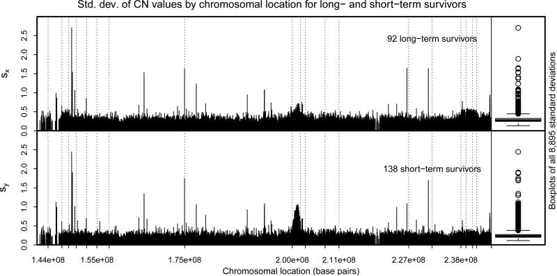
Figure 7 offers an explanation of the additional power demonstrated by the GCT. The upper and lower panels show the estimated standard deviation at each of the 8,895 copy number locations across the q arm of chromosome 1 for the 92 long-term and 138 short-term survivors, respectively. Both panels exhibit spikes at shared locations as well as prominent humps around 2.0 × 10⁸ Mbps, suggesting that the variances are not constant across the chromosome; nor are the humps at equal heights for the two groups of patients. The boxplots of the 8,895 standard deviations for each group reveal significant right skewness, suggesting heavy-tailedness of some of the component distributions. The minimum estimated standard deviations for the long- and short-term survivors were 0.1314 and 0.1123, respectively, indicating that the component variances are bounded sufficiently away from zero. The severe heteroscedasticity as well as the inequality of variances between the two samples appear to have attenuated the power of the Ch-Q and SK tests just as in the simulation.

Figure 7.

Sample standard deviations of copy number at all 8,894 copy number locations for long- and short-term survivors with boxplots at right. Gaps occur at chromosomal locations where no copy number measurements were taken. Vertical dashed lines delineate the twenty CBS-selected regions in which the equal means hypothesis was tested.

None of the univariate two-sample t-statistics in the lefthand panel of Figure 6 are very extreme, the largest of their magnitudes being 3.607. This suggests that the difference between the copy number profiles of short- and long-term survivors consists of smaller differences distributed over a larger number of components rather than larger differences over a smaller number of components. That is, the signals appear to be dense but weak rather than sparse but strong. In such a setting the CLX test will likely have low power.

It is worth discussing the computation time of the four tests. For this analysis, in which each test was implemented twenty times at various values of the dimension p, the moderate-p GCT finished in 1.75 seconds and the large-p GCT finished in 6.60 seconds. The Ch-Q and SK tests finished in 2.32 and 2.68 minutes, respectively, and the CLX took 2.79 hours to run on a MacBook Air with a 1.86 GHz Intel Core 2 Duo processor with 4 GB of memory. The SK procedure involves matrix operations which can be quite slow for large p, and the Ch-Q test involves a cross-validation type sum of inner products which becomes slow for large sample sizes. The CLX method must first test whether Σ₁ = Σ₂ and then directly estimate Σ^–1 or {Σ₁ + (n/m)Σ₂}^–1 under sparsity assumptions. Estimating these large matrices quickly becomes computationally burdensome. The GCT requires only a summation over p components and computation of the sample autocovariance function of a p-length series, making it very fast to compute.

6 Mitochondrial Calcium Concentration

Ruiz-Meana et al. (2003) subjected cells from cardiac muscles in mice to conditions which simulated reduced blood flow for a period of one hour. To a treatment group, a dose of cariporide was administered, which is believed to inhibit cell death due to oxidative stress. The investigators measured the mitochondrial concentration of Ca²⁺ every ten seconds during the hour. The experiment was run twice, once on intact cells and once on cells with permeabilized membranes. The data have been made available by Febrero-Bande & Oviedo de la Fuente (2012) in the R package fda.usc.

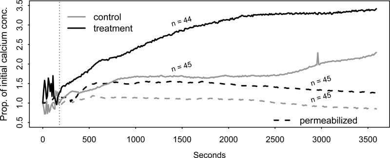
The mean percent increase of the calcium concentration over its initial value for the treatment and control in both the experiments is plotted against time in Figure 8, where the sample sizes for each curve are shown. The first 180 seconds of the data are removed, given the erratic behavior of the curves, leaving p = 342 time points. The four tests were applied to both the intact and permeabilized data to test for equality between the true treatment and control mean curves. The p-values for the four tests are given in Table 2.

Figure 8.

Mean curves of the proportional increase in calcium concentration over initial value in intact and permeabilized cells from cardiac muscles in mice over one hour with and without cariporide treatment. First 180 seconds removed from analysis.

Table 2.

The p-values produced by the four tests for equality between the treatment and control calcium concentration curves in the intact and permeabilized experiments.

	Ch-Q	SK	CLX	mod-p GCT	lg-p GCT
Intact	0.000	0.118	0.086	0.000	0.000
Permeabilized	0.001	0.358	0.817	0.000	0.000

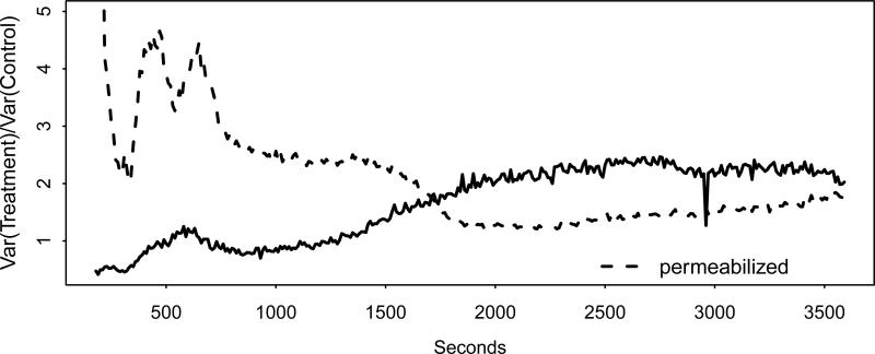
For the intact cells, the Ch-Q test and the GCT strongly rejected the null, while the CLX test, after failing to reject equality of the covariance matrices, produced a p-value of 0.086 under the equal covariances assumption, and the SK test failed to reject. For the permeabilized experiment the Ch-Q test and the GCT again strongly rejected the null. The CLX test again failed to reject equality of the covariance matrices, which is a dubious assumption for either the intact or permeabilized experiments given the plot in Figure 9 of $s_j^2∕{\vartheta }_j^2$ for j = 1, . . ., 342 for each set of data. In this plot the variance of the treatment group measurements for the intact cells is well over twice as high as in the control group for the first ten minutes (fluctuating wildly), and for the permeabilized cells the variance of the treatment group measurements remains at roughly twice that of the control group measurements after half an hour has elapsed. The low power of the SK test apparently owes to the variance inequality depicted here.

Figure 9.

Ratios of the variances of the proportional increase in calcium concentration for the treatment versus control group plotted against time for the intact and permeabilized data sets.

The inability of the CLX test to reject what appears to be an implausible null hypothesis likely owes to a difference in mean functions which is characterized by gradual separation rather than by spikes in one function or the other. The large number of small differences are unable to produce a maximum which will exceed the CLX rejection threshold. However, the Ch-Q test and the GCT are able to register the large number of small differences cumulatively and reject the equal means hypothesis.

This example illustrates the applicability of our test in functional data contexts, in which each observation consists of a function observed at points over some domain. When it is of interest to compare the mean functions in two populations, the assumptions of the GCT are likely to apply.

7 Conclusions

The test we present for H₀ : μ₁ = μ₂ versus H₁ : μ₁ ≠ μ₂, called the generalized component test, was shown to be competitive in the p > > n setting when the p components admit an ordering allowing the dependence between two components to be modeled according to their displacement. Moderate- and large-p versions of the test were given for p = o(n²) and p = o(n⁶), respectively. The test requires very little computation time and is easily scalable to very-large p settings.

The moderate-p version of our test is robust to ultra heavy-tailedness, and both the moderate- and large-p versions are robust to heteroscedasticity and highly unequal covariance matrices. The Chen and Qin (Ch-Q) test lost most of its power in the presence of heavy-tailedness or heteroscedasticity; the Srivastava and Kubokawa (SK) test lost much of its power when the covariance matrices were unequally scaled. The Cai, Liu, and Xia (CLX) test performed well under a variety of settings, proving to be robust to heteroscedasticity and to unequally scaled covariance matrices; however, when the data were very heavy-tailed, which rendered the signals very weak, the CLX lost considerable power. Also, since the CLX test requires estimating the p × p precision matrix, it is computationally much slower than the other tests, requiring over 2.5 hours to complete the copy number data analysis which the SK and Ch-Q tests completed in under 3 minutes and the GCT in under 10 seconds.

For the copy number analysis, the GCT exhibited superior power over the other three tests. This was likely due to heteroscedasticity in the component variances, under which the Ch-Q would lose power, unequally scaled variances between the two populations, under which the SK test would lose power, and likely to the presence of a dense-but-weak rather than a sparse-but-strong signal structure, under which the CLX test would have low power.

For the mitochondrial calcium concentration data set, only the Ch-Q test and the GCT were able to reject the equal means hypothesis. The SK test appears to have lost power due to unequal variances and the CLX supremum-based test was unable to detect the smooth separation of the two mean functions over time, which was characterized by small differences in many components rather than by large differences in a few.

Software

We created the R package highD2pop for implementing the GCT as well as the Ch-Q, SK, and CLX tests. A source version, highD2pop.zip, is available for download. The package includes copy number data for the CBS-selected segment of the q arm of chromosome 1 having p = 400 copy number probes. See package documentation in highD2pop-manual.pdf.

Figure 4.

Power curves at sample sizes (n, m) = (45, 60) for the moderate- and large-p GCT, Ch-Q, SK, and CLX tests against the proportion of nonzero mean differences β under IND, ARMA, and LR dependence (left to right) with heteroscedastic centered gamma(4, 2) innovations and Σ₂ = 2Σ₁. Based on S = 500 simulations.

Appendix: Proofs of main results

Proof 1 (Asymptotic Normality of Test Statistic) By an adaptation of the big-block-little-block argument to the triangular array it can be shown that $p^{-1∕2}{\sum }_{j=1}^p[t_{nj}^2-E{t}_{nj}^2]\to Normal(0,{\tau }_{\infty }^2)$, where

$$\begin{array}{cc}\hfill {\tau }_2^{\infty }=& \underset{n\to \infty }{\lim }Var\left(p^{-1∕2}\sum _{j=1}^p{t}_{nj}^2\right)=\underset{n\to \infty }{\lim }{p}^{-1}\sum _{k=0}^{p-1}\sum _{\mid j_1-j_2\mid =k}Cov(t_{n{j}_1}^2,t_{n{j}_2}^2)\hfill \\ \hfill =& \gamma \left(0\right)+2\sum _{k=1}^{\infty }\gamma \left(k\right),\hfill \end{array}$$ (A.1)

where $\gamma \left(k\right)={\lim }_{n\to \infty }{(p-k)}^{-1}{\sum }_{j=1}^{p-k}Cov(t_{nj}^2,t_{n(j+k)}^2)$, k ≥ 0. To prove (A.1), use the moment and α-mixing conditions to show that for any M ≥ 1,

$$\begin{array}{cc}\hfill p^{-1}\sum _{k=M+1}^{p-1}\sum _{\mid j_1-j_2\mid =k}\mid Cov(t_{n{j}_1},t_{n{j}_2})\mid \le & 2\sum _{k>M}{p}^{-1}(p-k)\left\{\alpha {\left(k\right)}^{\delta ∕(2+\delta )}\underset{j=1}{\overset{p}{\bigvee }}{\left(E{\mid t_{nj}\mid }^{2+\delta }\right)}^{\frac{2}{2+\delta }}\right\}\hfill \\ \hfill \le & C\sum _{k=M+1}^{\infty }\alpha {\left(k\right)}^{\delta ∕(2+\delta )}\to 0\hfill \end{array}$$

as M → ∞. Thus,

$$\begin{array}{cc}\hfill & \underset{x\in \mathbb{R}}{\sup }\mid P(\sqrt{p}[T_n-p^{-1}\sum _{j=1}^{p}E\left(t_{nj}^2\right)]\le x)-\Phi (x∕{\tau }_{\infty })\mid =o\left(1\right)\hfill \\ \hfill \Rightarrow & \underset{x\in \mathbb{R}}{\sup }\mid P(T_n-p^{-1}\sum _{j=1}^{p}E\left(t_{nj}^2\right)\ge x)-\Phi (\sqrt{p}x∕{\tau }_{\infty })\mid =o\left(1\right)\hfill \\ \hfill \Rightarrow & \underset{x\in \mathbb{R}}{\sup }\mid P(T_n-1\le x)-\Phi (\sqrt{p}[x-n^{-1}{a}_n-n^{-2}{b}_n]∕{\tau }_{\infty })\mid =o\left(1\right),\hfill \end{array}$$

where a_n and b_n are bounded sequences such that

$$p^{-1}\sum _{j=1}^{p}E\left(t_{nj}^2\right)=1+n^{-1}{a}_n+n^{-2}{b}_n+O\left(n^{-3}\right).$$ (A.2)

Lemma 1 provides c_nj and d_nj for j = 1, . . ., p such that a_n = (c_n1 + ··· + c_np)/p and b_n = (d_n1 + ··· + d_np)/p satisfy (A.2).

Lemma 1 Let X_1j, . . ., X_nj and Y_1j, . . ., Y_mj be independent identically distributed random samples with $Var\left(X_{1j}\right)={\sigma }_{1j}^2$ and $Var\left(Y_{1j}\right)={\sigma }_{2j}^2$ and EX_1j = EY_1j for all j = 1, . . ., p. Assume that max{E|X_1j|¹⁶, E|Y_1j|¹⁶, j = 1, . . ., p} = O(1) and that $\min \{{\sigma }_{1j}^2,{\sigma }_{2j}^2\}>c>0$ (The first moment condition may be reduced further by means of truncation, but this would considerably lengthen the proof. The discussion of heteroscedasitiy in Section 4.4 illustrates the importance of bounding the component variances away from zero). Let $t_{nj}^2=n{({\overline{X}}_{nj}-{\overline{Y}}_{mj})}^2{\{s_{nj}^2+(n∕m){\vartheta }_{mj}^2\}}^{-1}$, where $s_n^2$ and ${\vartheta }_m^2$ are the two samples variances and let m ~ n as n → ∞. Then $E\left(t_{nj}^2\right)=1+n^{-1}{c}_{nj}+n^{-2}{d}_{nj}+O\left(n^{-3}\right)$ for

$$c_{nj}={\tau }_{nj}^{-2}\{{\sigma }_{1j}^2+{(n∕m)}^2{\sigma }_{2j}^2\}+2{\tau }_{nj}^{-5}{\{{\mu }_{3j}^{\prime }+{(n∕m)}^2{\eta }_{3j}^{\prime }\}}^2$$ (A.3)

and

$$\begin{array}{cc}\hfill d_{nj}=& {\tau }_{nj}^{-4}[\{{\sigma }_{1j}^2+{(n∕m)}^2{\sigma }_{2j}^2\}-\{({\mu }_{4j}^{\prime }-3{\sigma }_{1j}^4)+{(n∕m)}^4({\eta }_{4j}^{\prime }-3{\sigma }_{2j}^4)\}]\hfill \\ \hfill +& {\tau }_{nj}^{-6}\{{\sigma }_{1j}^2+{(n∕m)}^2{\sigma }_{2j}^2\}\{({\mu }_{4j}^{\prime }-{\sigma }_{1j}^4)+{(n∕m)}^3({\eta }_{4j}^{\prime }-{\sigma }_{2j}^4)\}\hfill \\ \hfill -& 4{\tau }_{nj}^{-6}\{{\mu }_{3j}^{\prime }+{(n∕m)}^2{\eta }_{3j}^{\prime }\}\{{\mu }_{3j}^{\prime }+{(n∕m)}^3{\eta }_{3j}^{\prime }\}\hfill \\ \hfill -& {\tau }_{nj}^{-6}\{{\left({\mu }_{3j}^{\prime }\right)}^2+{(n∕m)}^5{\left({\eta }_{3j}^{\prime }\right)}^2\}\hfill \\ \hfill -& 6{\tau }_{nj}^{-8}\{{\mu }_{3j}^{\prime }+{(n∕m)}^2{\eta }_{3j}^{\prime }\}\{{\mu }_{5j}^{\prime }-2{\mu }_{3j}^{\prime }{\sigma }_{1j}^2+{(n∕m)}^4({\eta }_{5j}^{\prime }-2{\eta }_{3j}^{\prime }{\sigma }_{2j}^2)\}\hfill \\ \hfill -& 3{\tau }_{nj}^{-8}{\{({\mu }_{4j}^{\prime }-{\sigma }_{1j}^4)+{(n∕m)}^3({\eta }_{4j}^{\prime }-{\sigma }_{2j}^4)\}}^2\hfill \\ \hfill +& 6{\tau }_{nj}^{-8}\{{\sigma }_{1j}^2+{(n∕m)}^2{\sigma }_{2j}^2\}{\{{\mu }_{3j}^{\prime }+{(n∕m)}^2{\eta }_{3j}^{\prime }\}}^2\hfill \\ \hfill +& 3{\tau }_{nj}^{-10}\{{\sigma }_{1j}^2+(n∕m){\sigma }_{2j}^2\}{\{({\mu }_{4j}^{\prime }-{\sigma }_{1j}^4)+{(n∕m)}^3({\eta }_{4j}^{\prime }-{\sigma }_{2j}^4)\}}^2\hfill \\ \hfill +& 12{\tau }_{nj}^{-10}{\{{\mu }_{3j}^{\prime }+{(n∕m)}^2{\eta }_{3j}^{\prime }\}}^2\{({\mu }_{4j}^{\prime }-{\sigma }_{1j}^4)+{(n∕m)}^3({\eta }_{4j}^{\prime }-{\sigma }_{2j}^4)\},\hfill \end{array}$$ (A.4)

where ${\tau }_{nj}^2=\{{\sigma }_{1j}^2+(n∕m){\sigma }_{2j}^2\}$ and ${\mu }_{kj}^{\prime }$ and ${\eta }_{kj}^{\prime }$ are the kth central moments of X_1j and Y_1j, respectively.

Proof 2 (Proof of Lemma 1) For ease of syntax, ignore the subscript j, and, without loss of generality, assume that EX_1j = EY_1j = 0. Let ${\Delta }_n=s_n^2-{\sigma }_1^2+(n∕m)({\vartheta }_m^2-{\sigma }_2^2)$ and let $t_n^2$ be approximated by the expansion

$${\tilde{t}}_n^2=n{({\overline{X}}_n-{\overline{Y}}_m)}^2({\tau }_n^{-2}-{\tau }_n^{-4}{\Delta }_n+{\tau }_n^{-6}{\Delta }_n^2-{\tau }_n^{-8}{\Delta }_n^3+{\tau }_n^{-10}{\Delta }_n^4),$$ (A.5)

so that $t_n^2={\tilde{t}}_n^2+O_p\left(n^{-3}\right)$. An expression for the expected value $E\left({\tilde{t}}_{nj}^2\right)$ would thus involve the quantities $n{\tau }_n^{-2k}E{({\overline{X}}_n-{\overline{Y}}_m)}^2{\Delta }_n^{k-1}$ for k = 1, . . ., 5. These expectations must be computed such that they retain terms out to the order of O(n^–3).

Let χ_|B|({X_j : j ∈ B}) represent the joint cumulant of the random variables in the set {X_j : j ∈ B}, where |B| is the cardinality of B. Then the formula

$$E\left(X_1\dots X_k\right)={\Sigma }_{\pi }{\Pi }_{B\in \pi }{\chi }_{\mid B\mid }\left(\{X_j:j\in B\}\right)$$ (A.6)

from Leonov & Shiryaev (1959) gives the expected value of a product of random variables in terms of joint cumulants, where Σ_π denotes summation over all possible partitions of {X₁, . . ., X_k}, and Π_B∈π denotes the product over all cells of the partition π. Using (A.6) to compute $E{({\overline{X}}_n-{\overline{Y}}_m)}^2{\Delta }_n^{k-1}$ to within O(n^–4) of their true values for k = 1, . . ., 5 involves the joint cumulants tabulated below, where Δ ≡ Δ_n, X̄ ≡ X̄_n, and Ȳ ≡ Ȳ_m.

If κ(i, j) denotes the ijth member of the table of joint cumulants, then (A.6) gives

$$E{(\overline{X}-\overline{Y})}^2=\kappa (0,2)+O\left(n^{-4}\right)$$ (A.7)

$$E{(\overline{X}-\overline{Y})}^2\Delta =\kappa (1,2)+\kappa (0,2)\kappa (1,0)+O\left(n^{-4}\right)$$ (A.8)

$$E{(\overline{X}-\overline{Y})}^2{\Delta }^2=\kappa (2,2)+2\kappa (1,0)\kappa (1,2)+\kappa (0,2)\kappa (2,0)+2{\kappa }^2(1,1)+\kappa (0,2){\kappa }^2(1,0)+O\left(n^{-4}\right)$$ (A.9)

$$E{(\overline{X}-\overline{Y})}^2{\Delta }^3=\kappa (0,2)\kappa (3,0)+6\kappa (1,1)\kappa (2,1)+3\kappa (2,0)\kappa (1,2)+3\kappa (2,0)\kappa (1,2)+3\kappa (1,0)\kappa (2,0)\kappa (0,2)+6\kappa (1,0){\kappa }^2(1,1)+O\left(n^{-4}\right)$$ (A.10)

$$E{(\overline{X}-\overline{Y})}^2{\Delta }^4=3\kappa (0,2){\kappa }^2(2,0)+12{\kappa }^2(1,1)\kappa (2,0)+O\left(n^{-4}\right)$$ (A.11)

after removing cumulant products of order smaller than O(n^–4) and noting that κ(0, 1) = 0. Each cumulant is simplified using rules found in Brillinger (1981), and the formula

$${\chi }_k(X_1,\dots ,X_k){\Sigma }_{\pi }{(-1)}^{(\mid \pi \mid -1)}(\mid \pi \mid -1)!{\Pi }_{B\in \pi }E\left({\Pi }_{i\in B}{X}_i\right)$$ (A.12)

from Leonov & Shiryaev (1959) provides expressions for the simplified cumulants in terms of moments. Each cumulant is computed exactly or is approximated to within the order necessary for the cumulant products in (A.7)–(A.11) to lie within O(n^–4) of their true values. Two examples are worked out below.

$$\begin{array}{cc}\hfill \kappa (1,1)=& {\chi }_2(\Delta ,\overline{X}-\overline{Y})\hfill \\ \hfill =& {\chi }_2(\overline{X^2},\overline{X})-{\chi }_2(\overline{X^2},\overline{X})+(n∕m){\chi }_2(\overline{Y^2}-{\overline{Y}}^2,\overline{Y})\hfill \\ \hfill =& n^{-1}{\chi }_2(X_1^2,X_1)-n^{-3}{\chi }_2({\Sigma }_i{X}_i^2+{\Sigma }_{i\ne j}{X}_i{X}_j,{\Sigma }_j{X}_i)+(n∕m){\chi }_2(\overline{Y^2}-{\overline{Y}}^2,\overline{Y})\hfill \\ \hfill =& n^{-1}{\mu }_3^{\prime }-n^{-2}{\chi }_2(X_1^2+X_1{\Sigma }_{j=2}^n{X}_j,X_1)+(n∕m){\chi }_2(\overline{Y^2}-{\overline{Y}}^2,\overline{Y})\hfill \\ \hfill =& (n^{-1}-n^{-2}){\mu }_3^{\prime }+n^{-2}(n-1){\chi }_2(X_1{X}_2,X_1)+(n∕m){\chi }_2(\overline{Y^2}-{\overline{Y}}^2,\overline{Y})\hfill \\ \hfill =& (n^{-1}-n^{-2}){\mu }_3^{\prime }+(n∕m)(m^{-1}-m^{-2}){\eta }_3^{\prime }\hfill \end{array}$$

$$\begin{array}{cc}\hfill \kappa (2,0)=& {\chi }_2(\Delta ,\Delta )\hfill \\ \hfill =& {\chi }_2(\overline{X^2}-{\overline{X}}^2,\overline{X^2}-{\overline{X}}^2)+{(n∕m)}^2(\overline{Y^2}-{\overline{Y}}^2,\overline{Y^2}-{\overline{Y}}^2)\hfill \\ \hfill =& {\chi }_2(\overline{X^2},\overline{X^2})-2{\chi }_2(\overline{X^2},\overline{X^2})+{(n∕m)}^2{\chi }_2(\overline{Y^2}-{\overline{Y}}^2,\overline{Y^2}-{\overline{Y}}^2)\hfill \\ \hfill =& n^{-1}{\chi }_2(X_1^2,X_1^2)-2n^{-3}\{{\chi }_2({\Sigma }_i{X}_i^2,{\Sigma }_i{X}_i^2)+{\chi }_2({\Sigma }_{i\ne j},X_i{X}_j,{\Sigma }_i{X}_i^2)\}+n^{-1}\{{\chi }_2({\Sigma }_i{X}_i^2,{\Sigma }_i{X}_i^2)-2{\chi }_2({\Sigma }_{i\ne j}{X}_i{X}_j,{\Sigma }_j{X}_i^2)\}+n^{-4}{\chi }_2({\Sigma }_{i\ne j}{X}_i{X}_j,{\Sigma }_{i\ne j}{X}_i{X}_j)+{(n∕m)}^2{\chi }_2(\overline{Y^2}-{\overline{Y}}^2,\overline{Y^2}-{\overline{Y}}^2)\hfill \\ \hfill =& (n^{-1}-2n^{-2}+n^{-3})({\mu }_4^{\prime }-{\sigma }_1^4)+2(n-1)n^{-3}{\sigma }_1^4+{(n∕m)}^2{\chi }_2(\overline{Y^2}-{\overline{Y}}^2,\overline{Y^2}-{\overline{Y}}^2)\hfill \\ \hfill =& {(n-1)}^2{n}^{-3}{\mu }_4^{\prime }-(n-1)(n-3)n^{-3}{\sigma }_1^4+{(n∕m)}^2{\chi }_2(\overline{Y^2}-{\overline{Y}}^2,\overline{Y^2}-{\overline{Y}}^2)\hfill \\ \hfill =& (n^{-1}-2n^{-2}){\mu }_4^{\prime }-(n^{-1}-4n^{-2}){\sigma }_1^4+{(n∕m)}^2\{(m^{-1}-2m^{-2}){\eta }_4^{\prime }-(m^{-1}-4m^{-2}){\sigma }_2^4\}+\left(n^{-3}\right)\hfill \end{array}$$

Once all the cumulant expressions are obtained, they may be plugged into (A.7)–(A.11). Then, adding and subtracting (A.7)–(A.11) according to the expansion in (A.5) and gathering terms out of which n^–1 and n^–2 can be factored yields c_n from (A.3) and d_n from (A.4), respectively, which completes the proof.

References

- Anderson OD. Time Series Analysis and Forecasting: The Box-Jenkins Approach. Butterworths; 19 Cummings Park, Woburn, MA, 01801: 1977. [Google Scholar]
- Bai Z, Saranadasa H. Effect of high dimension: By an example of a two sample problem. Statistica Sinica. 1996;6:311–329. [Google Scholar]
- Baladandayuthapani V, Ji Y, Talluri R, Nieto-Barajas LE, Morris JS. Bayesian random segmentation models to identify shared copy number aberrations for array cgh data. Journal of the American Statistical Association. 2010;105:1358–1375. doi: 10.1198/jasa.2010.ap09250. [DOI] [PMC free article] [PubMed] [Google Scholar]
- Benjamini Y, Hochberg Y. Controlling the false discovery rate: a practical and powerful approach to multiple testing. Journal of the Royal Statistical Society. 1995;57:289–300. [Google Scholar]
- Benjamini Y, Yekutieli D. The control of the false discovery rate in multiple testing under dependency. The Annals of Statistics. 2001;29:1165–1188. [Google Scholar]
- Brillinger D. Holden-Day series in time series analysis. Holden-Day; 1981. Time Series: Data Analysis and Theory. [Google Scholar]
- Brockwell P, Davis R. Springer Series in Statistics. Springer; New York: 2009. Time Series: Theory and Methods. [Google Scholar]
- Cai T, Liu W, Luo X. A constrained l-1 minimization approach to sparse precision matrix estimation. Journal of the American Statistical Association. 2011;106:594–607. [Google Scholar]
- Cai T, Liu W, Xia Y. Two-sample covariance matrix testing and support recovery. Journal of the American Statistical Association. 2013;108:265–277. [Google Scholar]
- Cai TT, Liu W, Xia Y. Two-sample test of high dimensional means under dependence. J. R. Statist. Soc. B. 2014;76:349–372. [Google Scholar]
- Chen SX, Qin YL. A two sample test for high dimensional data with applications to gene-set testing. The Annals of Statistics. 2010;38:808–835. [Google Scholar]
- Febrero-Bande M, Oviedo de la Fuente M. Statistical computing in functional data analysis: The R package fda.usc. Journal of Statistical Software. 2012;51:1–28. [Google Scholar]
- Hall P, Jing B-Y, Lahiri SN. On the sampling window method for long-range dependent data. Statistica Sinica. 1998;8:1189–1204. [Google Scholar]
- Leonov VP, Shiryaev AN. On a method of calculation of semi-invariants. Theory of Probability and Its Applications. 1959;4:319–329. [Google Scholar]
- Olshen AB, Venkatraman ES, Lucito R, Wigler M. Circular binary segmentation for the analysis of array-based dna copy number data. Biostatistics. 2004;5:557–572. doi: 10.1093/biostatistics/kxh008. [DOI] [PubMed] [Google Scholar]
- Pang H, Liu H, Vanderbei R. fastclime: A fast solver for parameterized lp problems and constrained l1 minimization approach to sparse precision matrix estimation. R package version 1.2.3. 2013 [Google Scholar]
- Pinkel D, Albertson DG. Array comparative genomic hybridization and its applications in cancer. Nature Genetics Supplement. 2005;37:S11–S17. doi: 10.1038/ng1569. [DOI] [PubMed] [Google Scholar]
- Politis DN, Romano JP. Bias-corrected nonparametric spectral estimation. J. Time Ser. Anal. 1995;16:67–104. [Google Scholar]
- Ruiz-Meana M, Garcia-Dorado D, Pina P, Inserte J, Agulló L, Soler-Soler J. Cariporide preserves mitochondrial proton gradient and delays atp depletion in cardiomyocytes during ischemic conditions. Am J Physiol Heart Circ Physiol. 2003;285:H999–H1006. doi: 10.1152/ajpheart.00035.2003. [DOI] [PubMed] [Google Scholar]
- Seshan VE, Olshen A. DNAcopy: DNA copy number data analysis. R package version 1.36.0. 2013 [Google Scholar]
- Srivastava M. Multivariate theory for analyzing high dimensional data. J. Japan Statist. Soc. 2007;37:53–86. [Google Scholar]
- Srivastava MS, Kubokawa T. Tests for multivariate analysis of variance in high dimension under non-normality. Journal of Multivariate Analysis. 2013;115:204–216. [Google Scholar]
- Wu MC, Lee S, Cai T, Li Y, Boehnke M, Lin X. Rare-variant association testing for sequencing data with the sequence kernel association test. The American Journal of Human Genetics. 2011;89:82–93. doi: 10.1016/j.ajhg.2011.05.029. [DOI] [PMC free article] [PubMed] [Google Scholar]
- Wu Y, Genton MC, Stefanski LA. A multivariate two-sample test for small sample size and missing data. Biometrics. 2006;62:877–885. doi: 10.1111/j.1541-0420.2006.00533.x. [DOI] [PubMed] [Google Scholar]
Associated Data
This section collects any data citations, data availability statements, or supplementary materials included in this article.