Abstract
Small copy numbers of many molecular species in biological cells require stochastic models of the chemical reactions between the molecules and their motion. Important reactions often take place on one-dimensional structures embedded in three dimensions with molecules migrating between the dimensions. Examples of polymer structures in cells are DNA, microtubules, and actin filaments. An algorithm for simulation of such systems is developed at a mesoscopic level of approximation. An arbitrarily shaped polymer is coupled to a background Cartesian mesh in three dimensions. The realization of the system is made with a stochastic simulation algorithm in the spirit of Gillespie. The method is applied to model problems for verification and two more detailed models of transcription factor interaction with the DNA.
Keywords: Stochastic simulation, Chemical reaction, Diffusion, Mesoscale, Microscale
1 Introduction
Genetically identical cells can have very different phenotype. The explanation to this observation is that in addition to different environmental exposure, random fluctuations in gene expression are important (Elowitz et al. 2002; Metzler 2001; Munsky et al. 2012; Raj and van Oudenaarden 2008; Swain 2004). The reasons why there are random fluctuations are that the number of molecules involved in gene expression often is low, they have heterogeneous distribution in space and move randomly, and the chemical reactions occur with a certain probability when two molecules are in the vicinity of each other.
The DNA, microtubules, cytoskeletal fibers, and actin filaments are examples of one-dimensional (1D) structures or polymers embedded in the three-dimensional (3D) cytosol in a cell with important roles in the cell regulation, the signaling, and the transport of intracellular vesicles. In cell regulation, transcription factors find their specific site on the DNA by binding to a non-specific site, sliding on the DNA by 1D diffusion, dissociating from the DNA, diffusing in the cytosol, then rebinding to the DNA and finally finding the specific site in facilitated diffusion (Berg et al. 1981; Halford 2009; von Hippel and Berg 1989; Li et al. 2009). This process has been validated experimentally in Hammar et al. (2012). Motor proteins such as kinesin and dynein transport vesicles and organelles in a certain direction on the microtubule skeleton in eukaryote cells (Howard 1996; Kholodenko 2002; Mallik and Gross 2004; Vale 2003). The examples have in common that molecules can move on the polymers that can be modeled as 1D, diffuse in the ambient 3D space around the polymers, and react with other molecules on the polymers and in the cytosol.
In many cases, the only way to understand complex biochemical networks such as gene regulation is to use computer simulations. Macroscopic, deterministic models based on ordinary or partial differential equations for the concentrations of the chemical species will not capture crucial effects of these networks because of their inherent randomness. Stochastic modeling on a mesoscale is necessary where the discreteness and the intrinsic randomness of the systems are accounted for. The purpose of this paper is to develop a computational method for stochastic simulation of models of polymers submerged in the cytosol.
At a mesoscopic level of modeling, the spatial domain is partitioned into voxels or compartments and the state of the system is given by the copy numbers of the chemical species in each voxel. The molecules move by diffusion to neighboring voxels and react with other molecules in the same voxel. The probability density function (PDF) for the state of the system satisfies a reaction–diffusion master equation (RDME). The dimension of the domain of the solution is the number of voxels times the number of species. Except for very small systems, the RDME cannot be solved numerically due to the high dimension of the domain. A computationally feasible alternative is to generate trajectories of the system using Gillespie's Stochastic Simulation Algorithm (SSA) (Gillespie 1976), modifications of it for better computational efficiency (Cao et al. 2005, 2006; Gibson and Bruck 2000; Slepoy et al. 2008), or further developments suitable for space dependent problems (Drawert et al. 2010; Elf et al. 2003; Elf and Ehrenberg 2004; Marquez-Lago and Burrage 2007) and collect statistics for the moments of the distribution or to approximate the PDF. Space is discretized and the time for the next diffusion or reaction event is sampled from an exponential distribution. Software for Cartesian and unstructured spatial meshes is found in Drawert et al. (2012), Elf and Ehrenberg (2004), Engblom et al. (2009), Hattne et al. (2005), Hepburn et al. (2012). In Atzberger et al. (2007), a method is proposed for simulation of microscopic particles and chains in a fluid with thermal fluctuations. The difference compared to our work is that we are interested in the intrinsic noise due to diffusion and chemical reactions as modeled by the RDME with realizations of the process by the SSA.
A more accurate simulation is obtained with a microscopic model where the diffusion and reactions of single, individual molecules are tracked. The molecules move by Brownian motion and react with a certain probability when they are close. The diffusion is simulated by solving a stochastic differential equation for the position of the molecules using small timesteps in time-driven realizations in Andrews et al. (2010), Kerr et al. (2008). Another approach called Green's Function Reaction Dynamics (GFRD) is developed in van Zon and ten Wolde (2005) where the time to the next event is sampled from analytically defined or numerically computed probability distributions in event-driven realizations of the chemical systems. Space is continuous in implementations of the microscopic model in contrast to the mesoscopic model where space is discretized. The accuracy of the method is improved by introducing protective domains around the separate molecules in Donev et al. (2010), Takahashi et al. (2010). In recent work (Mauro et al. 2013; Hellander 2013), the single molecule simulation technique has been extended to 1D polymers embedded in 3D. Hybrid methods where some species are treated at the microscale and other species are modeled at the mesoscale are found in Flegg et al. (2012), Hellander et al. (2012a), Klann et al. (2012). For small voxel sizes at the meso level, there is a breakdown of the model compared to the microscopic model (Isaacson 2009). Corrections to mesoscopic reaction rate coefficients to avoid the breakdown are derived in Erban and Chapman (2009), Fange et al. (2010), Hellander et al. (2012b) from the probability distributions and the behavior at the micro level. The assumption is that the microscopic model is more accurate and that for a vanishing voxel size the mesoscopic model shall converge to the microscopic model.
An algorithm is developed in this paper to simulate biochemical systems at a mesoscopic level of approximation where there are stationary 1D structures such as polymers immersed in 3D space. Molecules react and diffuse in 3D and on the polymers and migrate between the 1D structures and 3D space. The algorithm is an extension of Gillespie's direct SSA (Gillespie 1976) and its adaptation to spatially dependent problems in the Next Subvolume Method (NSM) (Elf et al. 2003; Elf and Ehrenberg 2004). The 3D domain is covered by voxels organized in a Cartesian mesh. The geometry of the 1D structure is of arbitrary smooth shape and it is partitioned into subsegments independently of the background mesh for more generality. The state of the system is given by the time dependent copy numbers of the chemical species in each voxel in 3D and each subsegment in 1D. The coupling between the discretization in 3D and in 1D assumes that the distribution of the molecules is uniform inside the voxels and subsegments. The results of the simulations with the algorithm are compared to PDFs satisfying the partial differential equations of the microscopic level in examples with simple polymer geometries. The GFRD method in Hellander and Lötstedt (2011) is extended to curved 1D structures embedded in 3D and compared to mesoscopic simulations for a circular polymer. This method is further developed in Hellander (2013). The DNA and its interaction with transcription factors and repressors at a specific binding site are modeled in a bacterial cell using our method in the two final examples. Experimental and theoretical support for the DNA model is found in Berg et al. (1981), Halford (2009), Hammar et al. (2012), Li et al. (2009).
All parameters are given in SI-units, e.g. a length is in m, time is in s, reaction coefficients on the microscale are in m2/s or m3/s depending on the dimension, and a diffusion coefficient is in m2/s. Vectors and matrices are written in boldface. A vector u has the components ui and the elements of a matrix A are Aij. The Euclidean norm is denoted by ∥ · ∥. The biochemical and discretization parameters are collected in Tables 7 and 8 in the Appendix.
2 The Microscale Model
The Smoluchowski model (Smoluchowski 1917) with extended boundary conditions by Collins and Kimball (1949) is the governing equation for the PDF for the position of a molecule in space and for a reaction with another molecule. The molecules diffuse by Brownian motion and the reaction propensities are given by microscopic association and dissociation rates ka,micro, kb,micro and kd,micro, ku,micro. We discuss the equations for a molecule moving by diffusion in 3D space, a molecule moving by diffusion and reacting on 1D polymers, and a molecule binding to and dissociating from a 1D polymer. The microscale model is assumed to be more accurate than the mesoscale model described in the next section. As a verification of our mesoscale model and algorithm, the solutions of the microscale equations will be compared to the results from the mesoscale simulations. We do not consider the alternative model for the reactions due to Doi (1976) here. The Smoluchowski and the Doi models are compared in Agbanusi and Isaacson (2013).
2.1 Molecules in Three Dimensions
Assume that a single molecule A3 in free 3D space is at position x0 at time t0. The PDF for its position x at a later time t is p3(x, t|x0, t0). The molecule moves by Brownian motion with the diffusion coefficient D3. The PDF satisfies the diffusion equation
| (1) |
with initial condition
| (2) |
and a vanishing probability at ∞
| (3) |
Without boundaries and other molecules in the system, the PDF for the new position is a Gaussian
| (4) |
where Δt = t – t0. This is a model for a transcription factor A3 moving in the cytosol.
2.2 Diffusion and Reactions on the Polymer
Consider a one-dimensional polymer P with the arc length coordinate s ∈ [0, smax] and normal n. The radius of P is σ in the n-direction and it is embedded in 3D and has a smooth geometry. Molecules diffuse on P with diffusion coefficient D1 and may react with each other when they meet on P. A molecule cannot pass another molecule on the polymer. The PDF p1 (s, t|s0, t0) for the position of a molecule A1 on P starting at s0 at time t0 satisfies the diffusion equation in 1D
| (5) |
with initial condition
| (6) |
and Neumann boundary conditions at s = 0 and s = smax. This is a model for a transcription factor sliding on the DNA.
The reversible reaction between two species A1 and B on a polymer is
| (7) |
with the binding and unbinding coefficients kb,micro and ku,micro. Assume that B of length σB on P is located with its midpoint at sB and can react with many A1 and that A1 is in [sB + σB/2, smax]. The sum of the copy numbers of A1 and C is then constant. The boundary condition for p1 at sB + σB/2 is (cf. Kim and Shin 2000)
| (8) |
On the other side of B when A1 is in [0, sB – σB/2] then
| (9) |
In (sb – σB/2, sb + σB/2) we let p1(s, t|s0, t0) = 0. By conservation of A1 and C, the probability p1(*, t|s0, t0) that a C has been formed on P in (t0, t] and is present at sB at time t is given by
If kb,micro > 0 then the molecules can react with each other and when ku,micro > 0 they can be split apart. Here, A1 can be interpreted as a transcription factor on the DNA binding to and unbinding from the specific site.
The other molecule at sB serves as a roadblock for A1 when kb,micro = ku,micro = 0 in (8) and (9). Then A1 cannot pass B on the polymer.
2.3 Interaction with the Polymer
The free molecule A3 in Sect. 2.1 can react with P , diffuse on it and eventually dissociate from the polymer. When it is bound to P it is transformed to A1 and the association and dissociation reactions are
| (10) |
with the reaction coefficients ka,micro and kd,micro.
The PDF for A3 in 3D satisfies (1) if it is in free space and the PDF for A1 in 1D satisfies (5) if it is moving freely on P. Introduce a curvilinear coordinate system (r, ϕ, s) with r increasing in the normal direction from the polymer, ϕ being the azimuthal position, and s increasing along the polymer. Assume that σ is small. Then the boundary condition for (1) at the polymer is
| (11) |
The diffusion equation in (5) is modified with a source term due to the boundary terms in (11)
| (12) |
Equation (12) is derived by letting p1 be the integral of the 3D solution inside P over the circle of radius σ in the (r, ϕ)-plane. The second term on the right hand side is a good approximation if σ is so small that p3 can be considered independent of ϕ. Similar conditions are given in Berg and Ehrenberg (1982). There is an influx of A1 molecules to P depending on the density of A3 molecules at P in the second term in (12) and an outflux of A1 molecules in the third term in (12). The total probability density of A3 and A1 is conserved by (1), (11), and (12). This is a model for the interaction between a transcription factor and the DNA.
3 The Mesoscopic Model
In the mesoscopic model, the spatial domain of interest Ω is partitioned into voxels ωm, m = 1, . . . , M3, such that they are non-overlapping, , and they cover the domain, . The state of a space dependent chemical system at time t is given by the copy numbers of the species in each voxel. Molecules of two reacting species in the same voxel form a new compound with a certain probability and a molecule jumps to an adjacent voxel with a probability depending on the diffusion coefficient.
The domain is here a cube of size L × L × L with a Cartesian mesh aligned with the coordinate directions. The voxels ωijk, i, j, k = 1, . . . , N, are cubic with the edge length h implying that the total number of voxels is M3 = N3 where N = L/h. By letting m = N2(i – 1) + N(j – 1) + k, we have the general indexing in the paragraph above. The boundary conditions are reflective for the diffusion of the molecules at the boundary of Ω.
The discretization of the polymer is described in the next two subsections. Then the mesoscopic diffusion and reactions are found in the subsequent subsections corresponding to the microscopic model in Sects. 2.2 and 2.3. Finally, the algorithm is given and discussed.
3.1 Molecules in Three Dimensions
Consider a reversible reaction as in (7). In the mesoscopic model it is
| (13) |
The copy numbers of the species A, B, and C in voxel ωijk are denoted by aijk, bijk, and cijk, respectively. The reaction rate for the forward reaction is αf = ka,mesoaijkbijk and for the backward reaction αb = kd, mesocijk.
Molecular motion is modeled by transferring a=molecule in a voxel ωijk to one of its nearest neighbors in the x, y, and z directions ωi±1,j,k, ωi,j±1,k, or ωi,j,k±1. When A3 in ωijk diffuses to ωi,j,k+1, the change of the state can be written as a reaction
| (14) |
The diffusion rate αijk in the positive k-direction for a molecule A3 with copy number a3ijk in ωijk is D3a3ijk/h2.
Given these rates, one trajectory of the chemical system in Ω is simulated by the SSA (Gillespie 1976) or improvements of it suitable for spatial problems like the Next Subvolume Method (NSM) (Elf et al. 2003; Elf and Ehrenberg 2004). The time for the next event in the system is sampled from exponential distributions determined by the reaction and diffusion rates αf, αb, and αijk.
3.2 Discretization of the Polymer
Let the geometry of the polymer in 3D be given by
| (15) |
The polymer is discretized by approximating it with a polygon π(s). The corners of the polygon are at
| (16) |
see Fig. 1. The length of a straight subsegment ζm between sm–1 and sm on the polygon π(s) is
The polygon interpolates the polymer at ui such that γ (ui) = π(si) where si = si–1 + Δsi, i = 1, . . . , M1, s0 = 0 and si ≤ ui. If the discretization is equidistant with Δsj = Δs, then the diffusion rate for a jump of a molecule from subsegment ζj to ζj+1 or ζj-1 is D1/Δs2. If the subsegments have variable lengths, then the jump coefficients can be derived as in Engblom et al. (2009).
Fig. 1.

The polymer γ(u) (thick line) and its polygonal approximation π(s) (thin line) with M1 = 4
3.3 Mesoscopic Representation of the Polymer
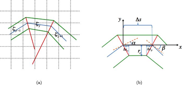
The subsegments ζj are surrounded by cylinders ηj for the coupling of the Cartesian mesh in Ω and the polygon π(s), see Fig. 2(a). The radius of ηj is rc and the surfaces at the top and bottom of the cylinder are planar. There is a plane defined by ζj–1 and ζj if they do not lie on a straight line. The bisector of ζj–1 and ζj through π(sj–1) specifies another plane which is orthogonal to . If ζj–1 and ζj are on the same straight line, then the normal of is given by ζj–1 or ζj . The intersections of the circular surface of ηj and the two orthogonal planes at π(sj–1) and at π(sj) define the end surfaces of ηj. The radius rc of ηj is chosen such that . In this way, the spatial resolution around the polymer is similar to the resolution in space.
Fig. 2.
(a) The discretized polymer (blue) is surrounded by a cylindrical surface (green) in the background mesh (dashed). The cylinders are separated by bisector planes (red). (b) Definition of the quantities for derivation of the curvature constraint for cylinder ηj
For ηj to be non-degenerate, rc has to be sufficiently small. Consider the planar configuration in Fig. 2(b). The curve γ (u) = (x(u), y(u)) with a constant z coordinate is approximately orthogonal to the perpendicular planes and bounding ηj from the left and the right. The derivatives of x(u) and y(u) with respect to u are denoted by xu and yu and xuj = xu(uj) and yuj = yu(uj). Then we have
Locally, let x(u) = u such that xu = 1 and x(uj) – x(uj–1) ≈ Δs. Then for a non-degenerate cylinder the requirement in Fig. 2(b) is
Hence, for small angles α and β the conclusion is that where k is the curvature of γ and Rγ is the radius of curvature. The radius of the cylinders should not exceed the radius of curvature of the polymer and the background mesh should be sufficiently fine to resolve the curved polymer.
3.4 Diffusion in Space
Diffusion in 3D between the voxels is modeled as a reaction in (14). A molecule A3ijk in ωijk can jump in six directions to the voxels ωi±1,j,k, ωi,j±1,k, ωi,j,k±1 with the rate D3a3ijk/h2.
3.5 Interaction with the Polymer
The reaction corresponding to (10) in the mesoscopic model for association with and dissociation from P is
| (17) |
The reaction rates in a voxel ωi and a subvolume ηj are determined by the coefficients ka,meso and kd,meso and the copy numbers of A3 and A1. Let Vji denote the volume of the overlap between ηj and ωi. Most Vji are zero. The volumes of ηj and ωi are and Vi = |ωi| = h3, respectively. By the definition of the volumes we have
| (18) |
The first relation in (18) is also an equality if ωi is completely covered by cylinders ηj but most voxels have no overlap with the cylinder around polymer and the sum is zero.
The association reaction rate in ηj due to A3 molecules in ωi is denoted by λ3ji. The total rate in voxel i is λ3i and the total rate in subvolume j is . The copy number of A3 in ωi is a3i and there is one copy of P in (17). The expressions for the association rates are
| (19) |
by (18) and assuming a uniform distribution of A3 in ωi. The rate for an associative event in ωi is λ3i and the probability that A3 is attached to ηj is λ3ji/λ3i.
The dissociation rate in ωi due to molecules A1 on the polymer in ηj is λ1ij and the total rates in ωi and ηj are λ1i and , respectively. With the copy number of A1 in ηj denoted by a1j, the dissociation rates are by (18)
| (20) |
The dissociation rate in ηj is kd,mesoa1j as expected and the probability that A1 is released into ωi is . Conversely, if an A1 molecule is released into ωi, then the probability that it came from ηj is λ1ij/λ1i.
3.6 Diffusion on the Polymer
Diffusion in 3D between the voxels is modeled as a reaction in (14). On the polymer, an A1 molecule moves from ηj to ηj±1 with the rate αj± in
| (21) |
The diffusion coefficient αj± is D1/Δs2 if the lengths of the subsegments are identical. Let the diffusion rate in ωi be δi,j± due to a1j molecules of species A1 in ηj. The accumulated diffusion rate in ωi is denoted by δi and the total diffusion rate in ηj is . These rates are derived in the same way as in (20)
| (22) |
| (23) |
If there is a diffusion event in ωi, then it takes place in ηj with probability (δi,j– + δi,j+)/δi. The probability is equal to leave ηj to the left and to the right .
Crowding on the polymer is modeled by not allowing two molecules to occupy the same subsegment. If ηj–1 or ηj+1 is selected for a jump from ηj and another molecule already resides in the chosen subsegment then the jump is canceled.
3.7 Reactions on the Polymer
The reaction when A1 binds and unbinds to the stationary site B on the polymer corresponding to (7) is
| (24) |
Suppose that at least one A1 and the B site are located in subvolume ηk. Then the rate for A1 to bind to B in ωi is λbik and the total rate for A1 to bind is λbk. With a1k molecules in ηk the propensities are
| (25) |
With the same definitions of λuik and λuk for the unbinding of A1 from B as in (25) for the binding event, the rates are with ãk A1 molecules bound to B
| (26) |
3.8 Total Rates
The propensity for a reaction event to take place in ωi is by (19), (20), (25), and (26)
| (27) |
The propensity for a diffusion event in ωi is the diffusion propensity in 3D plus the diffusion on the polymer in (22). If all ζj are of equal length, then the propensity is
| (28) |
The total propensity for an event in ωi is then
| (29) |
The incremental time ti for the next reaction or diffusion event in ωi is exponentially distributed with rate αi and is computed as ti = –logξ/αi where ξ is uniformly distributed in [0, 1].
If an event occurs in ωi, it is a reaction event with probability αRi/αi and a diffusion event with probability αDi/αi. If there is a reaction event then the probability that it is an association to the polymer is λ3i/αRi, a dissociation from the polymer λ1i/αRi, a binding event to the B site λbik/αRi, and an unbinding event λuik/αRi. The probability that a diffusion event in ωi is diffusion in 3D space is 6D3a3j/αDi and diffusion on the polymer δi/αDi.
3.9 The Algorithm
The algorithm for generating one trajectory of a chemical system with an embedded one-dimensional structure is a modification of the original NSM (Elf et al. 2003; Elf and Ehrenberg 2004). Suppose that an event i with probability λi consists of several possible alternatives such as reactions and diffusion jumps with rates λij and λi = Σj λij. If event i has occurred, one of the alternatives is chosen with probability λij/λi by sampling ξ ∈ [0, 1] from a uniform distribution. Take alternative k if
| (30) |
The algorithm is based on the derivations above and is as follows:
Algorithm: Modified Next Subvolume Method
Initialize the number of molecules in the voxels and subvolumes at t = 0.
Compute the reaction propensity function αRi (27), the diffusion propensity function αDi (28), and total propensity function αi for each voxel.
Sample the exponentially distributed time ti to the first reaction or diffusion event in voxel i with the rate αi in (29).
Find the smallest value among ti, i = 1, . . . , M3, and denote it by tk. Then the next event occurs in voxel k at time t := t + tk.
Sample as in (30) to determine if a chemical reaction or a diffusion event occurs in voxel k, see Sect. 3.8.
- If a chemical reaction event occurs:
- Sample as in (30) the chemical reaction that will take place, see Sect. 3.8.
- Update the number of molecules in voxel k and in subvolume j accordingly.
- Recalculate the propensity functions αRi and αDi and the time to the next event for the voxels involved in the reaction and, if there is a reaction on the polymer, the voxels that overlap the sampled subvolume.
- If a diffusion event occurs:
- Sample as in (30) the molecular species that diffuses to an adjacent voxel or subvolume, see Sect. 3.8.
- If there is diffusion in space:
- Sample as in (30) one of the six directions to determine the index of the voxel k′ to which the molecule diffuses, see Sect. 3.4.
- Update the number of molecules in voxels k and k′ accordingly.
- Recalculate the propensity functions αRi and αDi and the time to the next event for voxels k and k′.
- If there is diffusion on the polymer:
- Sample as in (30) the subvolume ηj and direction – or + with probability δk,j–/δk or δk,j+/δk, see Sect. 3.6.
- Update the number of molecules in subvolumes ηj and ηj–1 or ηj+1 accordingly.
- Recalculate the propensity functions αRi and αDi and the time to the next event for voxels ωi which overlap subvolumes ηj and either ηj–1 or ηj+1.
Find the smallest value among ti, i = 1, . . . , M3, and denote it by tk. Then the next event occurs in voxel k at time t := t + tk. If t < T go back to step (5), otherwise stop.
The NSM algorithm in Elf et al. (2003) is modified in steps 6b, 6d, and 7c to handle reactions involving the polymer and molecular motion on it. The method is stable in the sense that with only diffusion events, the total number of molecules is preserved.
The common volume Vji of voxel ωi and subvolume ηj is often rather complicated to compute by a deterministic method. An alternative is to approximate the volume by Monte Carlo integration. In a voxel ωi close to the polymer, generate uniformly distributed random numbers and count the number of them also inside ηj and divide by the total number in ωi yielding an estimate of Vji/Vi.
The algorithm is here given for two overlapping meshes, one Cartesian mesh in 3D for molecules in space and one cylindrical mesh in 1D for the polymer, but it can be generalized to any overlapping meshes. For example, suppose that we have a curved membrane represented by surface mesh consisting of triangles. Then create a volume mesh with one layer of prisms. A prism in the mesh has a surface triangle as the base and another triangle as the top with triangle corners connected by three edges along the normals of the surface. Reactions between molecules in the voxels in the background Cartesian mesh and the subvolumes in the prism mesh are then modeled in the overlapping region between the prismatic subvolumes and the cubic voxels. The copy numbers of the species in a prism are determined by the overlap between the prism and the neighboring voxels in the same manner as it is determined for the cylinder surrounding the polymer. The rates for reactions with the membrane are then computed using the copy numbers in the prisms. A method for deriving diffusion jump coefficients for membranes in Cartesian meshes is found in Isaacson and Peskin (2006). Using a mesh consisting of one layer of prisms at the membrane would be an alternative to that method.
Given some intrinsic microscopic reaction rates ka,micro and kd,micro, we need to transform them to the corresponding mesoscopic reaction rates ka,meso and kd,meso in order for the mesoscopic model to behave as the microscopic model. For large voxels in 3D the correct formulas are given by Collins and Kimball (1949), Fange et al. (2010)
However, no corresponding formulas exist for a larger lattice size in 2D. For small voxels in 3D and for simulations in 2D, the mesoscopic reaction rates will be mesh dependent. Mesoscopic reaction rates for diminishing h in 3D have been derived in Erban and Chapman (2009), Fange et al. (2010), Hellander et al. (2012b) and mesoscopic reaction rates in 2D have been derived in Fange et al. (2010), Hellander et al. (2012b). The two formulas in Fange et al. (2010) and Hellander et al. (2012b) give similar results for larger h, but different results for smaller h. This is because the formulas are derived from different microscopic modeling assumptions. In our numerical experiments in Sect. 4 we have used the conversion formulas in Hellander et al. (2012b), which give accurate results for our problems.
The conversion formula in Hellander et al. (2012b) is derived by matching the mean association time for two molecules diffusing on a Cartesian mesh with periodic boundary conditions. First, without loss of generality, assume that one of the molecules is fixed at the origin, and that the other molecule has a uniform initial distribution. The average time until the molecules react at the microscopic level, τmicro, is derived in Fange et al. (2010) and the average time until the molecules react at the mesoscopic level, τmeso, can be derived as in Hellander et al. (2012b). By choosing the mesoscopic reaction rate such that τmeso = τmicro, the average reaction time at the mesoscopic level will match the average reaction time at the microscopic level.
The conversion formula is given by
| (31) |
where M is the number of voxels M3 = N3 in 3D or the number of surface patches N2 in 2D and τD is the average time for the two molecules to diffuse to the same voxel or surface patch at the mesoscopic level. Asymptotic expressions for τD in two and three dimensions are derived in Montroll and Weiss (1965), Montroll (1969).
4 Results
As a verification of the Algorithm in Sect. 3, we first compare mesoscopic simulations with numerical solutions of the microscopic equations in Sect. 2. The microscopic model is more detailed following separate molecules, with a continuous space and a more advanced reaction model. When the fidelity and accuracy of the mesoscopic model are evaluated it is compared to the microscopic model e.g. in Erban and Chapman (2007), Fange et al. (2010), Isaacson (2009). Then a mesoscopic model of diffusion on the DNA and its vicinity in the cytosol and a specific binding of transcription factors to the DNA is proposed based on the theoretical and experimental evidence in Hammar et al. (2012), Li et al. (2009). The definitions of the physical and computational parameters are collected in the Appendix.
4.1 A Straight Polymer
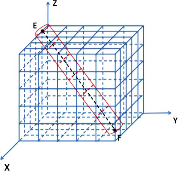
A mesoscopic model of a straight polymer P along the diagonal of Ω between E = (0, 0, L) and F = (L, L, 0) is illustrated in Fig. 3. By placing P on the diagonal, a better test of the generality of the algorithm is constructed than having P aligned with an axis of the coordinate system. The line segment consists of identical subsegments ζi surrounded by cylindrical subvolumes ηi in red.
Fig. 3.
Mesoscopic model of the polymer represented by a straight line segment (dashed black) between E and F with N = 5 and M1 = 6 and surrounded by a=cylinder (red) in the Cartesian mesh (blue)
The Algorithm is employed to generate realizations of the reaction–diffusion process for three different initial distances r0 between the polymer and the A molecules. To compute the volume intersections Vji, we take advantage of the special geometry of the polymer in this model by using cylindrical coordinates with the cylindrical z-axis along P . By discretizing the line into identical subsegments, the sub-volumes in the interior are identical cylinders with radius and height where Ls is the length of the diagonal. The computational and physical parameters in the simulations are found in Table 1. In the mesoscopic simulation, ka,meso = 3.94 × 10⁻¹³ per area in the discretization in 2D or 3.94 × 10⁻¹³/h2 = 17.5115 by the conversion formula in Hellander et al. (2012b) and kd,meso is chosen such that kd,micro/ka,micro = kd,meso/ka,meso. The time interval is [0, T] = [0, 0.1] at both levels of approximation. The parameter σ is the radius of polymer and is defined in Sect. 2.3.
Table 1.
Parameters in Sect. 4.1
| Variable | Value | Variable | Value | Variable | Value | Variable | Value |
|---|---|---|---|---|---|---|---|
| M 1 | 35 | N | 20 | L | 3 × 10⁻⁶ | h | 1.5 × 10⁻⁷ |
| k a,micro | 5 × 10–13 | k d,micro | 5 × 10–13 | k a,meso | 17.5115 | k d,meso | 17.5115 |
| D 3 | 10–12 | D 1 | 10–12 | σ | 1.005 × 10⁻⁹ |
4.1.1 Intermediate Distance
At t0 = 0, 104 molecules of species A3 in (10) are released in the voxel ωi with midpoint coordinate (0.475L, 0.525L, 0.525L). In the microscopic model, the molecule A3 is placed initially at a distance r0 = 1.2247 × 10⁻⁷ from P equal to the distance from the midpoint of ωi to the polymer. In this case, r0 ≈ 0.8h.
Introduce cylindrical coordinates (r, ϕ, s) around P in the microscopic model with s along the cylinder. The PDF satisfies the Smoluchowski equation (1) with boundary condition (11). The distribution pr(r, t|r0, t0) in the r-direction satisfies the Smoluchowski equation in 2D
| (32) |
with initial condition
| (33) |
and boundary conditions
| (34) |
| (35) |
In (35), . The initial position of the molecule is at r0 in (33). The probability for the molecule to be far away from P vanishes (34), and (35) is the boundary condition for association to P and dissociation from P . The probability that the molecule is at r0 initially and on the polymer at t is denoted by pr(*, t|r0, t0). It is defined by pr for r > σ and is related to p1 in (12) by a scaling β as follows:
The Smoluchowski equation (32), (33), (34), and (35) is solved numerically with a second order finite difference formula.
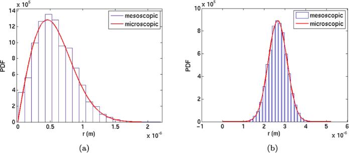
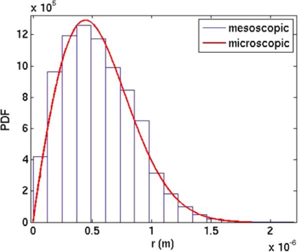
One hundred trajectories of the mesoscopic model are generated for 104 independent molecules and advanced until T = 0.1. The space outside the straight polymer P is partitioned into concentric cylinders between ri–1 and ri where ri = ri–1 + Δr, i = 1, . . . , R, for some R with r0 = 0. If the center of the voxel ωj with aωj molecules is in then aωj is added to the total number of molecules in . Each is a bin in the histogram in Fig. 4(a) with height proportional to . The scaling ϑ of the height is such that
| (36) |
The distribution of the molecules at T is compared to 2πrpr with pr from (32) in Fig. 4(a).
Fig. 4.
The distributions of molecules obtained by mesoscale simulations (blue) and the microscopic Smoluchowski equation (red) at time T = 0.1 with an intermediate initial distance to the polymer. (a) Distribution of molecule A3 in the radial direction. (b) Distribution of molecule A1 on P
The number of A1 molecules on the polymer is zero initially. By diffusion in space and the source terms in (12), the number of A1 grows on P. The diffusion in space and along the polymer has the same rate and the distribution of A1 will be Gaussian ~ exp(–(s – s0)2/4D1T) where s0 is the s-coordinate on P for the release of the A3 molecules. The mesoscopic data are scaled such that the area of the histogram equals 1 (cf. (36)) and is equal to the integral of the Gaussian in Fig. 4(b). Here the boundaries in the bins in the histogram are s0 ± i Δς, i = 0, 1, 2, . . . for some positive Δς. The agreement is very good between the mesoscale and microscale models in Fig. 4.
The average number of A1 in the mesoscopic model at T = 0.1 is 284.88. In the microscopic model, the probability of finding a molecule A3 in free space is 0.9715. Hence, the probability pr(*, t|r0, t0) of finding a molecule on P is 0.0285 and the expected copy number of A1 is 285. The relative error in the mesoscopic copy number of A1 compared to the microscopic number is much less than one percent.
4.1.2 Longer Distance
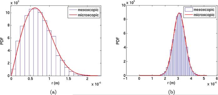
The starting position has a larger r0 in this experiment. In the mesoscopic simulation, 104 molecules of A3 are placed in the voxel with midpoint at (0.725L, 0.525L, 0.525L). The equivalent initial position in the microscopic model is r0 = 4.8990 × 10⁻⁷ ≈ 3.3h. The other parameters are the same as in Sect. 4.1.1 and Table 1. The comparisons are displayed at T = 0.1 in Fig. 5. The scaling of the histogram in Fig. 5(a) is as in (36) and in Fig. 5(b) it is the same as in Fig. 4(b).
Fig. 5.
The distributions of molecules obtained by mesoscale simulations (blue) and the microscopic Smoluchowski equation (red) with a longer initial distance to the polymer. (a) Distribution of molecule A3. (b) Distribution of molecule A1 on P
A good agreement between the mesoscopic and the microscopic models is observed again. The copy number a1 of A1 predicted by the microscopic solution is 74. In the mesoscopic simulation, the number of A1 is 74.17.
The dependence of a1, taken as the average over a number of samples, on Δs = Ls/M1 is found in Table 2. The variation is due to the Monte Carlo simulation with the number of samples used here and in this range of M1 a1 appears to be insensitive to Δs but the resolution of the distribution of A1 on P is less accurate for small M1.
Table 2.
The number of A1 molecules for different discretizations of the polymer
| M 1 | 25 | 30 | 35 | 40 | 45 |
| a 1 | 73.72 | 74.38 | 74.17 | 73.77 | 74.26 |
4.1.3 Short Distance
In order to test the sensitivity in the mesoscale model to the spatial resolution near the polymer, 104 A3 molecules are initially located in a voxel with a midpoint on the polymer at (0.525L, 0.525L, 0.525L) with the shortest distance to the polymer in the experiments. The smallest possible value of r0 in the microscopic model is σ implying that initially A3 touches the polymer but no association with the polymer has yet occurred.
The PDFs obtained from the mesoscopic and the microscopic models with r0 = σ do not agree very well. The copy number of A1 is 1921 in the microscopic model and 400.82 in the mesoscopic model. The discrepancy is explained by the assumption of having a uniform distribution of A3 in a voxel. For high precision in the initial position in the mesoscopic model, the voxels have to be small in the vicinity of the polymer. This is necessary when r0 is small since the microscopic PDF is sensitive to r0. Instead of refining the mesh, an average distance from the polymer ravg is determined for molecules in the voxel with the initial distribution of A3. Then take r0 = ravg in the Smoluchowski equation. The average distance is calculated by a Monte Carlo method with 104 coordinates inside the voxel resulting in ravg = 5.5987 × 10⁻⁸ ≈ 0.4h. A much better agreement is then observed in Fig. 6 in the comparison between the PDFs computed by the mesoscopic and the microscopic models. The distribution of A1 is Gaussian as in Figs. 4 and 5. The copy number of molecule A1 is 381 in the microscopic model and 400.82 in the mesoscopic model. The remaining difference between the microscopic and the mesoscopic models on P is caused by the lack of spatial resolution at the meso level and the imprecise initial position at the micro level.
Fig. 6.
The distributions of A3 molecules obtained by mesoscale simulations (blue) and the microscopic Smoluchowski equation (red) with a short initial distance to the polymer in the microscopic model
4.2 Two Parallel Polymers
Two straight polymers are studied in this example with two different association rates ka. The purpose is to see how the PDF in space is influenced by the presence of the polymers. The line segments can be located anywhere inside the simulation domain Ω in our algorithm for the mesoscopic model. There are many A-molecules in the system and they all move in 3D as A3, attach to the polymer as A1, and diffuse there independently. However, the governing PDE in the microscopic model is rather complicated to solve numerically with an arbitrary orientation of the polymers. By restricting the configuration to two parallel line segments, the Smoluchowski equation can be solved by a finite difference method in a bipolar coordinate system (Arfken 1970, p. 97) where the boundary condition (11) is applied at one coordinate being two different constants corresponding to the radius r = σ of the two polymers. With a low association rate, this is possible without numerical difficulties but for a high rate with more visible effects of the polymers, a major numerical effort would be necessary.
4.2.1 The Microscopic Model
The Smoluchowski equation is solved in the bipolar cylindrical coordinate system (u, v, y) (Arfken 1970, p. 97) defined by
| (37) |
where u ∈ [0, 2π], v ∈ (–∞, ∞) and y ∈ (–∞, ∞). It follows from the identities below that the curves of constant u and v are circles in the xz-plane:
| (38) |
| (39) |
Equation (39) defines a circle whose center is at (a coth v, 0) with the radius a csch v. Thus, by choosing appropriate values of a and v we have two cylinders in the 3D space and can apply the boundary conditions at the polymer surfaces at v = ±vc.
With the distance between the cylinders equal to L/q, the equations to solve for vc are
| (40) |
with solutions
| (41) |
The governing PDE in the uv-space is (see Arfken 1970, p. 76)
| (42) |
with initial condition
| (43) |
and boundary conditions for an associative event
| (44) |
where
| (45) |
The finite domain is (u, v) ∈ [0, 2π] × [–vc, vc].
The Smoluchowski PDE above is solved numerically with a second order finite difference method on a Cartesian grid in the uv-plane.
4.2.2 Low Association Rate
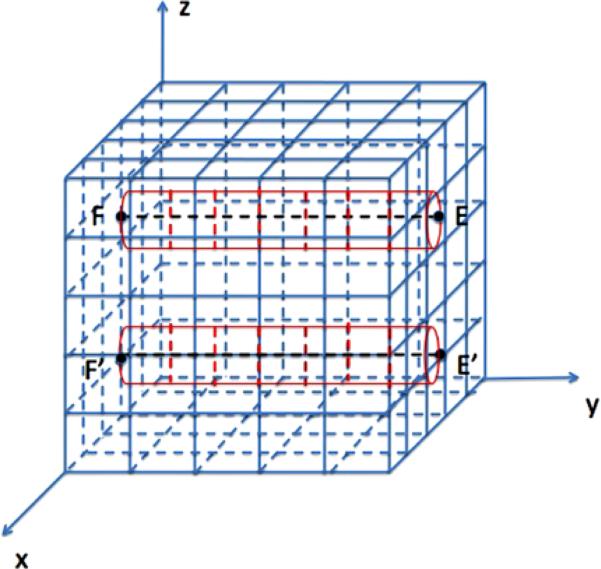
The results in this section obtained from mesoscopic simulations and the microscopic PDE solution are compared with respect to the distribution of the molecules. The model parameters are displayed in Table 3. The molecules cannot dissociate, kd,micro = 0, from the polymers of length Ls = L in this example. The end coordinates of the two segments are E = (L/2, L, 2L/3), F = (L/2, 0, 2L/3), and E′ = (L/2, L, L/3) and F′ = (L/2, 0, L/3), see Fig. 7. The distance between the polymers is L/3 implying that q = 3 in (40).
Table 3.
Parameters in Sect. 4.2
| Variable | Value | Variable | Value | Variable | Value | Variable | Value |
|---|---|---|---|---|---|---|---|
| M 1 | 20 | N | 20 | L | 3 × 10⁻⁶ | h | 1.5 × 10⁻⁷ |
| k a,micro | 5 × 10–13 | k d,micro | 0 | k a,meso | 17.5115 | k d,meso | 0 |
| D 3 | 10–12 | D 1 | 10–12 | σ | 1.005 × 10⁻⁹ | T | 0.1 |
Fig. 7.
The mesoscopic model with two polymers E F and E′ F′ and space discretization with N = 5 and M1 = 7
The initial position of the molecule is (u, v, y) = (π, 0, L/2) in the microscopic model at the midpoint of Ω and between the polymers. Since there is no voxel with its midpoint at (π, 0, L/2) when N is even, 104 molecules are uniformly distributed in the eight voxels surrounding the midpoint of Ω. The results using 104 molecules in one trajectory are equal to the simulation of one molecule in 104 trajectories since the molecules are independent. As in Sect. 4.1, the rate per h2 is ka,meso = 17.5155 using the 2D formula in Hellander et al. (2012b) and kd,meso is chosen to be 0. The assumption in Hellander et al. (2012b) is that there is only one straight polymer in Ω but the conversion formula is accurate as long as the interaction between the two polymers here is weak.
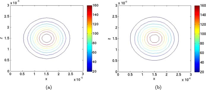
The PDE (42) with boundary conditions (44) is solved numerically in the uv-plane and transferred to the xz-system in Fig. 8(a). The solution is almost a Gaussian distribution as we would have if there were no polymers. The reason is that the association rate is low. The numbers of molecules in the columns of voxels parallel to the polymers in the y-direction are summed in the N × N grid in the xz-plane and displayed in Fig. 8(b) after scaling. The level curves are similar with both methods. At the v boundaries, the functions g1 and g2 in (45) are singular at two points when u ∈ [0, 2π] calling for a very fine mesh or special treatment there for good accuracy.
Fig. 8.
Isolines of the PDF in the xz-plane around the two polymers at (1.5, 1) × 10–6 and (1.5, 2) × 10–6. (a) Solution of the Smoluchowski equation. (b) Solution using the mesoscopic model
4.2.3 High Association Rate
In this experiment, the values of the parameters are the same except for a larger association rate in order to observe perturbations in the Gaussian distribution around the polymers. We choose ka,micro = 5 × 10⁻⁷ yielding ka,meso = 82.6965. These values are not realistic in a real living cell but are used to test the algorithm. Without a major effort, the numerical solution of the Smoluchowski equation cannot be obtained for this ka,micro due to the strict requirements on the mesh close to the polymers and the stiffness there.
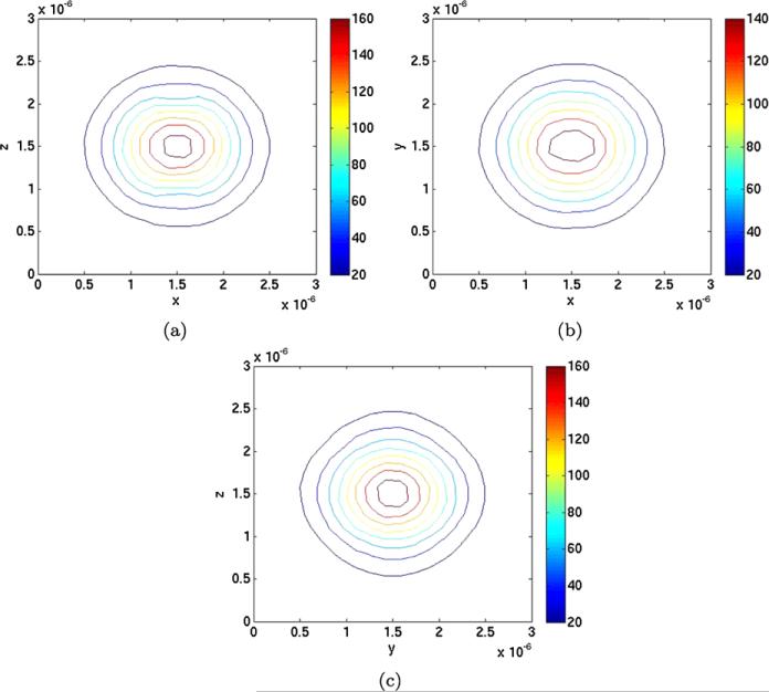
The distribution of A3 from the mesoscopic simulations is displayed in Fig. 9 in projections in the xz-plane, the xy-plane, and the yz-plane. In Fig. 9(a), the perturbations are observed around the (x, z) points (1.5, 1) × 10–6 and (1.5, 2) × 10–6 which are the positions of the polymers. The perturbation along a single polymer is accumulated along the y-axis to make it sufficiently large to be visible. The perturbations along the polymer in Figs. 9(b) and 9(c) are not as clear as in Fig. 9(a). An even larger association rate is needed to observe the perturbations of the Gaussian there. However, there is an upper limit of the association rate in the mesoscopic model (Erban and Chapman 2009; Hellander et al. 2012b). Our ka,meso is quite close to that limit and cannot be increased much for a more visible effect.
Fig. 9.
Isolines of the projected PDF obtained by mesoscopic simulations in different planes around the two polymers. (a) xz-plane. (b) xy-plane. (c) yz-plane
4.3 Arbitrarily Oriented Polymers
In this section, the Algorithm is applied to more complicated polymer configurations. The polymer is a circle in the first example and a spiral in the second one. The microscopic association and dissociation rates and the numerical parameters are shown in Table 4. The assumption is also here that the conversion formulas from the microscale to the mesoscale coefficients are accurate despite the fact that they are derived for a polar coordinate system instead of a general, curved system.
Table 4.
Parameters in Sect. 4.3
| Variable | Value | Variable | Value | Variable | Value | Variable | Value |
|---|---|---|---|---|---|---|---|
| N | 20 | L | 3 × 10⁻⁶ | h | 1.5 × 10⁻⁷ | ||
| k a,micro | 5 × 10–13 | k d,micro | 5 × 10–13 | k a,meso | 17.5115 | k d,meso | 17.5115 |
| D 3 | 10–12 | D 1 | 10–12 | σ | 1.005 × 10⁻⁹ |
A finite difference solution of the PDE in Sect. 2.1 for the circle is possible using a toroidal coordinate system (Arfken 1970, p. 112) and a finite element solution around the spiral using an unstructured mesh is also viable but would require substantial implementation and computational efforts for accurate solutions due to the small σ compared to L. Mesoscopic simulation and averaging over many trajectories as in Fig. 8(b) are an alternative way of obtaining approximations of the PDFs satisfying the Smoluchowski equation. A computational effort is still necessary using mesoscopic simulation but the Algorithm is easily programmed and the mesh generation is simple.
4.3.1 Circle
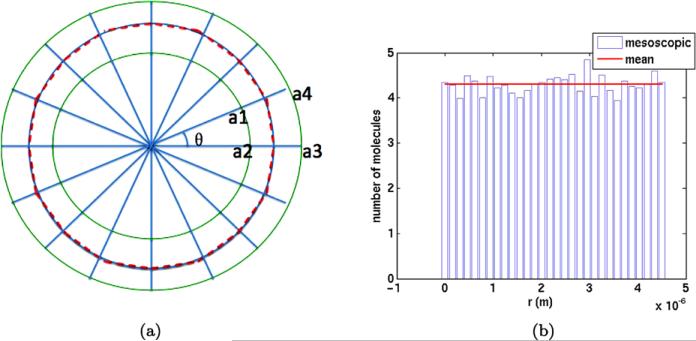
A circular polymer with radius ρ is embedded in 3D space. The mesoscopic discretization of it is found in Fig. 10(a). The projection in the circle plane of a cylindrical subvolume ηi around the segment ζi is defined by the quadrilateral with the corners a1, a2, a3, a4. The quotients Vji/Vi and Vji/Vj in Sect. 3.3 are calculated by a Monte Carlo method utilizing the special structure of the circle.
Fig. 10.
(a) A circle (dashed red) in 2D and its discretization into subsegments and subvolumes (green). (b) A histogram of the number of molecules A1 on the circle and the average number
The radius of the circle is ρ = 0.239L. The center coincides with the midpoint of Ω. The number of subvolumes and subsegments M1 is 30 with θ = 2π/M1 and Δs = 2ρ sin(θ/2). At t = 0, 104 independent A3 molecules are uniformly distributed in the eight voxels around the midpoint of Ω. The distribution is close to uniform at T = 0.1 in Fig. 10(b) as expected by symmetry.
To compare results obtained with the mesoscopic simulations to the corresponding microscopic model we have also simulated the system according to the version of the GFRD algorithm described in Hellander (2013), Hellander and Lötstedt (2011). The new position of a molecule or a reaction is sampled from a probability distribution with a PDF satisfying a Smoluchowski equation.
A torus is generated by letting a circle with radius σ = 1.005 × 10⁻⁹ revolve around the circle defined as above. There is no known analytical solution for the PDF for a single molecule in space interacting with a torus. Although it would be possible to solve the corresponding Smoluchowski equation numerically with for instance a finite difference method, it would be fairly complicated and involve a substantial computational effort as noted above. Instead, the molecules diffuse in free space until they are within a distance d to the torus. If the distance is larger than d, we choose a time step Δt and update the positions of the molecules by sampling from a normal distribution as in (4). Let the distance of a molecule to the torus be dcyl. To ensure that the molecules are unlikely to react with the torus during this time step, we choose Δt such that the standard deviation of the normal distribution is much smaller than dcyl.
When a molecule is close to the torus and d > dcyl, the torus is approximated by a straight cylinder. The algorithm in Hellander and Lötstedt (2011) is then directly applicable using the 2D Smoluchowski equation (32) to determine the PDF to sample a new position from. Since σ is much smaller than the radius ρ of the circle, this will be a good approximation for a sufficiently short time. This methodology works also for more general polymers. We have chosen d = 4σ and for dcyl > d. For d > dcyl, we choose Δt = 10–4 and sample a new distance to the torus by solving the Smoluchowski equation (32) numerically with a finite difference method. During this time step the molecule can react with the torus.
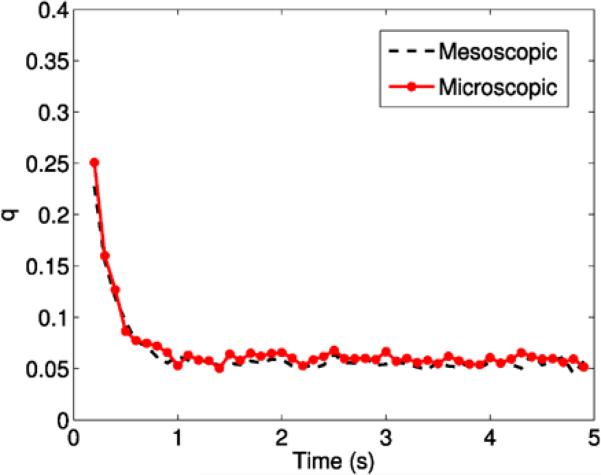
The system is simulated until time T = 4.9 s, with ka,micro as in Table 4 and kd,micro = 0. We have then computed, mesoscopically and microscopically, the effective reaction rate q, defined as the proportion of free molecules A3 having reacted with the torus per second and become A1 for discrete time points t < T. The molecules are initially placed uniformly in the eight voxels surrounding the midpoint of the domain. As we can see in Fig. 11, this affects the effective rate initially, since the molecules start close to the circle. After about a second, they have had time to spread in the domain, and the rate settles and is constant throughout the rest of the simulation, as expected. The mesoscopic and microscopic simulations are in good agreement.
Fig. 11.
Comparison between the effective reaction rate q in mesoscopic and microscopic simulations
4.3.2 Spiral
A more general geometry is a spiral γ (u) = (x(u), y(u), z(u))T defined by the coordinates
| (46) |
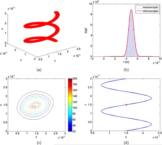
where 0 ≤ u ≤ 4π. The cylinder of radius rc with the polymer in the center is depicted in Fig. 12(a) by plotting dots at the coordinates used in the Monte Carlo evaluation of Vji/Vj. The spiral is a general structure of the polymer.
Fig. 12.
(a) Volume rendering of the cylinder around the spiral by the sample points in the Monte Carlo integration. (b) The PDF of A1 on the spiral. (c) A projection of the PDF of A3 in the yz-plane. (d) Projection of the geometry in the yz plane with initial position of the A1 molecules (red)
The number of subvolumes M1 on the spiral after discretization is 66. The volumes of ωi and ηj are approximately equal. The other parameters are in Table 4. Initially, 104 molecules of species A1 are placed on the spiral in a subvolume whose midpoint coordinates are (0.7477L, 0.4763L, 0.4924L).
The distribution of A1 on the polymer is shown in Fig. 12(b). The histogram is the result of the mesoscopic simulation and the red curve is a Gaussian ~ exp(–(s – s0)2/4D1T) where s0 is the s-coordinate for the release of the A molecules. The copy number of A3 is projected in the yz-plane in Fig. 12(c). The distribution is close to normal but slightly perturbed along the spiral. An explanation is given by comparing the PDF with the projected geometry of the spiral in Fig. 12(d). The A1 molecules are initialized at the red spot. The spread of A1 in Fig. 12(b) is about 2 × 10⁻⁶. Then the expected perturbation of the spatial distribution occurs on the line between (y, z) = (0.8, 1.2) × 10–6 and (2.2, 1.7) × 10–6. This is what we observe in Fig. 12(c).
4.4 Diffusion with Roadblocks
The polymer P models a part of a bacterial DNA strand in this example. A transcription factor A diffuses in space as A3, is bound non-specifically to the DNA as A1, diffuses on the DNA, and when A1 is at the specific binding site B it can react with B. The diffusion of A1 on P is blocked by repressor roadblocks R1 which cannot be passed in one dimension (Li et al. 2009). The repressor molecules either have a fixed position on P or move by diffusion on P. The transcription factor can dissociate from the DNA and associate with other parts of the DNA in its search for the specific binding site by facilitated diffusion (Berg et al. 1981; Hammar et al. 2012; von Hippel and Berg 1989). In a living cell, the copy number of each transcription factor is low. We are interested in the time when an initially free transcription factor binds to the specific binding site and when an initially bound transcription factor leaves the neighborhood of the section of the DNA where it was bound.
4.4.1 Fixed Roadblocks
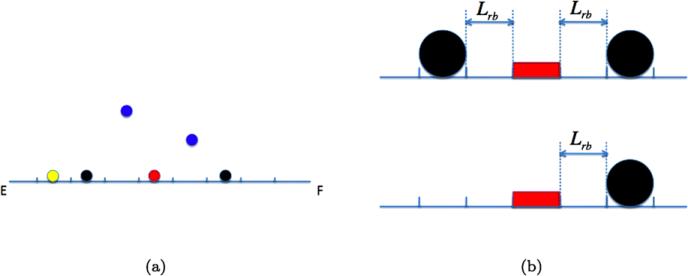
The domain Ω and its discretization are the same as in the previous sections. The DNA is modeled as a straight, diagonal polymer P denoted by E F in Fig. 13(a). The polymer is partitioned into identical subsegments. A specific binding site B is located on P at a fixed position with one or two fixed roadblocks of species R1, see Fig. 13(a). The distance between B and R1 is Lrb in Fig. 13(b). Transcription factors A3 diffuse in space and may be attached to DNA in a non-specific binding. When a transcription factor A1 is bound to the DNA, it diffuses along the DNA, and binds to B but it cannot pass the roadblocks. It may also be released from P and return to 3D space as A3. The association, dissociation, binding, and unbinding events are characterized by the following reactions:
| (47) |
where ka and kd are the association and dissociation rates to P and kb and ku are the rates for the binding and unbinding of the transcription factor A1 to the specific binding site B where they form the compound AB.
Fig. 13.
(a) The DNA as a polymer between E and F and a specific binding site B (red). The transcription factors A3 in space (blue) in the same plane as the DNA and A1 on DNA (yellow) and two fixed roadblocks R1 (black). (b) The distance Lrb between the specific site B (red) and two fixed roadblocks (black) (top) and one fixed roadblock (bottom)
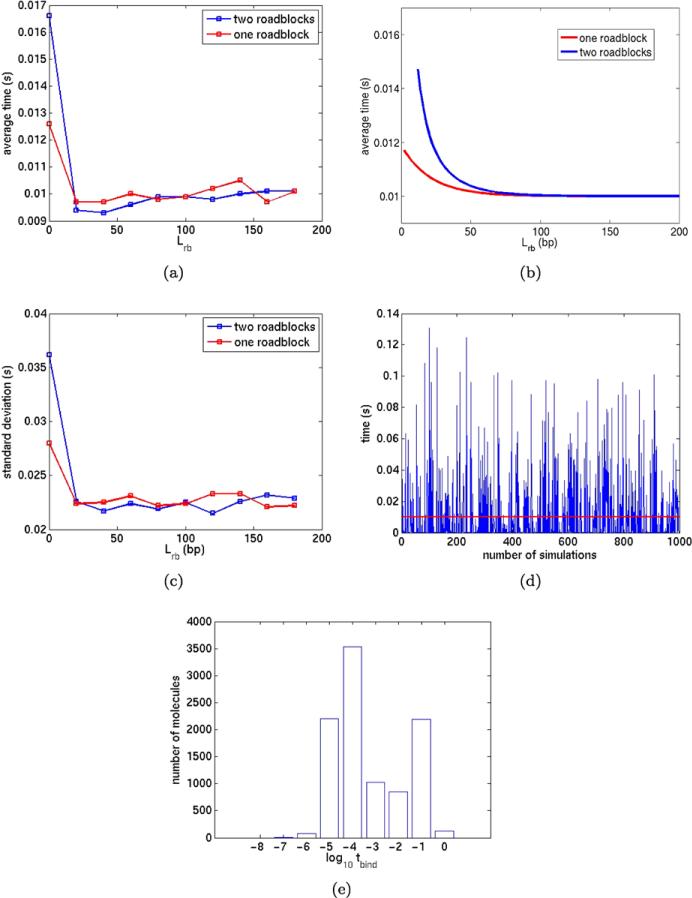
We are interested in the time tbind it takes for a free A3 to bind to the specific site B and how tbind varies with Lrb. The binding time tbind is the biologically relevant time for locating and binding a chromosome operator site from free diffusion in the cytoplasm. The time will increase significantly if the operator is positioned between two closely spaced DNA binding proteins at Lrb from the site. The distance represents the crowding of proteins on chromosomal DNA and the relation to tbind reflects how the crowding influences the search time for an operator.
In the numerical experiment, the coordinates of the diagonal line segment are E = (0, 0, L) and F = (L, L, 0), where L is the side length of the cube Ω, see Fig. 3. The parameters in the experiment are tabulated below.
For each value of Lrb, we simulate the time tbind and analyze how tbind depends on Lrb. In each simulation, 10 molecules A3 are initialized in the voxel with the midpoint (0.475L, 0.475L, 0.475L). This voxel overlaps with the subvolume with B. We expect a short binding time since the initial position of the transcription factor is close to the specific binding site. The length of a subsegment is where bp is one base pair on DNA. The length of one bp is 0.34 × 10⁻⁹ (Watson and Crick 1953).
In Fig. 14(a), the average value of tbind for one and two roadblocks in 104 realizations is shown with the corresponding value of Lrb given in bp. For Lrb greater than the average sliding distance , tbind is about 0.01 with one or two roadblocks. According to the theory in Hammar et al. (2012, Supplement, p. 31) the average binding times with one and two roadblocks, tbind1 and tbind2, are
| (48) |
where γ = kb,meso/D1 and in the length unit bp and is the binding time when Lrb → ∞.
Fig. 14.
(a) The average value of tbind in the mesoscale simulation for two roadblocks (blue) and one roadblock (red) for different distances Lrb. (b) The theoretical value of tbind in Hammar et al. (2012) for two roadblocks (blue) and one roadblock (red) for different distances Lrb. (c) The standard deviation of tbind for two roadblocks (blue) and one roadblock (red) for different distances Lrb. (d) The binding time tbind in 1000 consecutive realizations with Lrb = 120bp (blue) and the average time (red). (e) The histogram of tbind in logarithmic scale in 104 realizations with Lrb = 120bp
The analytical values of tbind in (48) are plotted in Fig. 14(b) with and the parameter values in Table 5 for comparison with the numerical experiments in Fig. 14(a). The agreement is good with one roadblock but for two roadblocks the theory predicts higher tbind. When Lrb = 0 then tbind2 = 0.17 in theory. In the simulations, the result for small Lrb is sensitive to the precise conditions at the specific site, the spatial resolution (Δs = 20bp here) around it, and the initial position of the molecules. The standard deviation in tbind is quite large in Fig. 14(c), even larger than the average of tbind. As an example, take Lrb = 120bp. Then the large variation in tbind is apparent in Fig. 14(d). The PDF of tbind is approximated in Fig. 14(e) by a histogram with data from 104 trajectories. A majority of the binding times are very short and there is another peak at the mean value. The initial position of the transcription factor is close to the DNA here. Randomly chosen coordinates for it at t0 would increase tbind and probably lower the variation.
Table 5.
Parameters in Sect. 4.4.1
| Variable | Value | Variable | Value | Variable | Value | Variable | Value |
|---|---|---|---|---|---|---|---|
| M 1 | 35 | N | 20 | L | 1.36 × 10⁻⁷ | h | 0.68 × 10⁻⁸ |
| k a,micro | 5 × 10–13 | k d,micro | 5 × 10–13 | k a,meso | 1.057 × 10⁴ | k d,meso | 1.057 × 10⁴ |
| D 3 | 10–12 | D 1 | 10–12 | σ | 1.005 × 10⁻⁹ | k b,meso | 2 × 10⁵ |
4.4.2 Moving Roadblocks
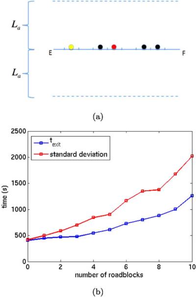
Transcription factors move along DNA by sliding as can be seen in direct single molecule experiments in vitro (Blainey et al. 2009; Elf et al. 2007) and indirect single molecule experiment in living cells (Hammar et al. 2012). It has also been shown these molecules cannot bypass other molecules on chromosomes in living cells. Sliding diffusion barriers on DNA were first introduced in Li et al. (2009) to account for the 1D crowding effects caused by the high occupancy of DNA binding proteins sliding on DNA and searching for different binding sites. Therefore, the repressor roadblock molecule R1 diffuses on the DNA in this more elaborate model as illustrated in Fig. 15(a).
Fig. 15.
(a) The repressors R1 on DNA acting as moving roadblocks (black), and a transcription factor A1 (yellow) released from B (red). (b) The exit time texit in 1000 simulations for different number of repressors R1 on DNA
The simulation domain Ω and its discretization are the same as in Sect. 4.4.1. The straight polymer P modeling the DNA is here located on a line parallel to one of the coordinate axes.
A roadblock R1 or a transcription factor A1 occupies Ms subsegments in this example with Ms > 1. If R1 or A1 occupies one subsegment, then it blocks also the neighboring ⌊(Ms – 1)/2⌋ subsegments to the left and ⌈(Ms – 1)/2⌈ to the right for other A1 or R1. Both A1 and R1 cover MsΔs. This is a way of simulating crowding in 1D with molecules of length Msδs on the DNA and not allowing molecules to pass each other. In the mesoscopic Algorithm in Sect. 3, the new restriction is that a molecule A1 or R1 cannot enter a subsegment of P already occupied by another molecule. The only modification of the algorithm in this example is that a molecule bound to P covers Ms subsegments of P instead of only one subsegment. The reactions are the same as in (47). For a good resolution of the DNA M1 = 400 and Δs = 1bp in this case. Since the length of transcription factors on the DNA is about 20bp we take Ms = 20.
At t0 = 0, the bond between A1 and B is broken and A1 diffuses away from B or rebinds to B. The molecule A1 is initially in the same subsegment as B. We are interested in the elapsed time texit for A1 to dissociate from P to become A3 and leave a cylinder C of radius La around P. It may rebind to B several times before it leaves the neighborhood of this part of the DNA strand and approaches another one outside C. The roadblocks R1 diffuse on the DNA and stay there and the copy number of them vary in the experiments. Their initial positions at t0 = 0 are chosen from a uniform distribution on the polymer. The molecules involved in=the model are depicted in Fig. 15(a).
The parameters in this example are found in Table 6. By the formulas in Hellander et al. (2012b), the mesoscopic rates scaled by 1/h2 are in the table satisfying kd,micro/ka,micro = kd,meso/ka,meso for this discretization of the domain and the polymer. The unbinding rate ku,meso of A1 from the specific site is chosen such that the mean time of existence of the complex AB is 60 s. The voxel size h is 6.8σ for the conversion of ka,micro to ka,meso in Hellander et al. (2012b) to be applicable. The exit radius La is 2h = 1.36 × 10⁻⁸.
Table 6.
Parameters in Sect. 4.4.2
| Variable | Value | Variable | Value | Variable | Value | Variable | Value |
|---|---|---|---|---|---|---|---|
| M 1 | 400 | N | 20 | L | 1.36 × 10⁻⁷ | h | 0.68 × 10⁻⁸ |
| k a,micro | 5 × 10–13 | k d,micro | 2.5 × 10⁻¹⁴ | k a,meso | 1.0731 × 10⁴ | k d,meso | 540.39 |
| D 3 | 3 × 10–12 | D 1 | 4.6 × 10⁻¹⁴ | σ | 1.0 × 10⁻⁹ | k b,meso | 2 × 10⁵ |
The system is simulated until texit for different number r1 of R1 molecules. The average texit from 1000 trajectories is found in Fig. 15(b). After an association reaction A1 + B → AB, the transcription factor is bound to the site for 60 s and is then released and can diffuse again on the DNA or in space. The average time increases slowly for small r1 and increases, as it seems, faster than linearly for larger r1. When r1 = 10 the repressors occupy half the space on the DNA. Most of the variation in the elapsed time for different r1 is due to rebinding events to the specific site. With more repressors on the DNA, the transcription factor on the DNA returns to the binding site more often because of more roadblocks impeding its motion on the DNA.
5 Discussion
A method for simulation of stochastic, mesoscopic models in molecular biology has been developed where diffusion and reactions on one-dimensional structures are embedded in three-dimensional space. The NSM (Elf et al. 2003; Elf and Ehrenberg 2004) for Cartesian meshes is modified to include polymers such as DNA of general geometrical shape in the simulation. The statistics from realizations of simple mesoscopic models are compared to the PDFs for the same microscopic models with good agreement. The method is applied to a model to study the effect of roadblocks in the vicinity of a specific binding site on the DNA and the time it takes for a transcription factor to find the site or the time it takes for it to leave the neighborhood of the DNA.
The mesh is Cartesian in the examples, but the Algorithm is applicable also to an unstructured 3D mesh. The computation of the overlap volumes Vji in Sect. 3.3 is then slightly more complicated but this is the only difference. Reactions and diffusion on two-dimensional surfaces such as membranes can be handled in a similar manner as one-dimensional lines but would require some algorithmic extensions. The geometries of the polymers are assumed to be constant in time here. The simulation of moving polymers and surfaces with reactions and diffusion on them is a more complicated computational problem.
Acknowledgements
This work has been supported by the Swedish Research Council (SH, SW), the European Research Council (JE), and the NIH grant for StochSS with number 1R01EB014877-01 (SH).
Appendix
Table 7.
Biochemical parameters in Sect. 4
| D3 | diffusion coefficient in 3D space |
| D1 | diffusion coefficient on the 1D polymer |
| ka,micro | coefficient for association of A3 to P in the microscopic model |
| kd,micro | coefficient for dissociation of A1 from P in the microscopic model |
| ka,meso | coefficient for association of A3 to P in the mesoscopic model |
| kd,meso | coefficient for dissociation of A1 from P in the mesoscopic model |
| kb,micro | coefficient for binding of A1 to B in the microscopic model |
| ku,micro | coefficient for unbinding of A1 from B in the microscopic model |
| kb,meso | coefficient for binding of A1 to B in the mesoscopic model |
| ku,meso | coefficient for unbinding of A1 from B in the mesoscopic model |
Table 8.
Discretization parameters in Sect. 4
| Ω | the cubic domain |
| ωi | voxel i in the mesh |
| ζj | subsegment j on the polymer |
| ηj | subvolume j surrounding ζj |
| N | number of voxels in each coordinate direction of the cube |
| M3 | total number of voxels, M3 = N3 |
| M1 | number of subsegments on the polymer |
| L | length of an edge of the cube |
| Ls | length of the polymer in the cube |
| h | length of an edge of a voxel, h = L/N |
| Δs | length of a subsegment on P |
Contributor Information
Siyang Wang, Division of Scientific Computing, Department of Information Technology, Uppsala University siyang.wang@it.uu.se.
Johan Elf, Division of Computational and Systems Biology, Department of Cell and Molecular Biology, Science for Life Laboratory, Uppsala University, P.O. Box 596, 75124 Uppsala, Sweden johan.elf@icm.uu.se.
Stefan Hellander, Division of Scientific Computing, Department of Information Technology, Uppsala University stefan.hellander@it.uu.se.
Per Lötstedt, Division of Scientific Computing, Department of Information Technology, Uppsala University.
References
- Agbanusi IC, Isaacson SA. A comparison of bimolecular reaction models for stochastic reaction diffusion systems. Bull. Math. Biol. 2013 doi: 10.1007/s11538-013-9833-6. (to appear) [DOI] [PubMed] [Google Scholar]
- Andrews SS, Addy NJ, Brent R, Arkin AP. Detailed simulations of cell biology with Smoldyn 2.1. PLoS Comput. Biol. 2010;6(3):e1000705. doi: 10.1371/journal.pcbi.1000705. [DOI] [PMC free article] [PubMed] [Google Scholar]
- Arfken G. Mathematical methods for physicists. 2nd ed. Academic Press; Orlando: 1970. [Google Scholar]
- Atzberger PJ, Kramer PR, Peskin CS. A stochastic immersed boundary method for fluid-structure dynamics at microscopic length scales. J. Comput. Phys. 2007;224:1255–1292. [Google Scholar]
- Berg OG, Ehrenberg M. Association kinetics with coupled three- and one-dimensional diffusion: chain-length dependence of the association rate to specific DNA sites. Biophys. Chem. 1982;15:41–51. doi: 10.1016/0301-4622(82)87015-4. [DOI] [PubMed] [Google Scholar]
- Berg OG, Winter RB, von Hippel PH. Diffusion-driven mechanisms of protein translocation on nucleic acids, 1: models and theory. Biochemistry. 1981;20:6929–6948. doi: 10.1021/bi00527a028. [DOI] [PubMed] [Google Scholar]
- Blainey PC, Luo G, Kou SC, Mangel WF, Verdine GL, Bagchi B, Xie XS. Nonspecifically bound proteins spin while diffusing along DNA. Nat. Struct. Mol. Biol. 2009;16:1224–1229. doi: 10.1038/nsmb.1716. [DOI] [PMC free article] [PubMed] [Google Scholar]
- Cao Y, Gillespie DT, Petzold LR. The slow-scale stochastic simulation algorithm. J. Chem. Phys. 2005;122:014116. doi: 10.1063/1.1824902. [DOI] [PubMed] [Google Scholar]
- Cao Y, Gillespie DT, Petzold LR. Efficient step size selection for the tau-leaping simulation method. J. Chem. Phys. 2006;124:044109. doi: 10.1063/1.2159468. [DOI] [PubMed] [Google Scholar]
- Collins FC, Kimball GE. Diffusion-controlled reaction rates. J. Colloid Sci. 1949;4:425–437. [Google Scholar]
- Doi M. Stochastic theory of diffusion-controlled reaction. J. Phys. A. Math. Gen. 1976;9(9):1479–1495. [Google Scholar]
- Donev A, Bulatov VV, Oppelstrup T, Gilmer GH, Sadigh B, Kalos MH. A first-passage kinetic Monte Carlo algorithm for complex diffusion–reaction systems. J. Comput. Phys. 2010;229:3214–3236. [Google Scholar]
- Drawert B, Lawson MJ, Petzold L, Khammash M. The diffusive finite state projection algorithm for efficient simulation of the stochastic reaction–diffusion master equation. J. Chem. Phys. 2010;132(7):074101. doi: 10.1063/1.3310809. [DOI] [PMC free article] [PubMed] [Google Scholar]
- Drawert B, Engblom S, Hellander A. URDME: a modular framework for stochastic simulation of reaction-transport processes in complex geometries. BMC Syst. Biol. 2012;6:76. doi: 10.1186/1752-0509-6-76. [DOI] [PMC free article] [PubMed] [Google Scholar]
- Elf J, Ehrenberg M. Spontaneous separation of bi-stable biochemical systems into spatial domains of opposite phases. Syst. Biol. 2004;1:230–236. doi: 10.1049/sb:20045021. [DOI] [PubMed] [Google Scholar]
- Elf J, Dončić A, Ehrenberg M. Bezrukov SM, Frauenfelder H, Moss F, editors. Mesoscopic reaction–diffusion in intracellular signaling. Proc. SPIE: Vol. 5110. Fluctuations and noise in biological, biophysical, and biomedical systems. 2003:114–124. [Google Scholar]
- Elf J, Li G-W, Xie XS. Probing transcription factor dynamics at the single-molecule level in a living cell. Science. 2007;316(5828):1191–1194. doi: 10.1126/science.1141967. [DOI] [PMC free article] [PubMed] [Google Scholar]
- Elowitz MB, Levine AJ, Siggia ED, Swain PS. Stochastic gene expression in a single cell. Science. 2002;297(5584):1183–1186. doi: 10.1126/science.1070919. [DOI] [PubMed] [Google Scholar]
- Engblom S, Ferm L, Hellander A, Lötstedt P. Simulation of stochastic reaction–diffusion processes on unstructured meshes. SIAM J. Sci. Comput. 2009;31:1774–1797. [Google Scholar]
- Erban R, Chapman SJ. Reactive boundary conditions for stochastic simulations of reaction– diffusion processes. Phys. Biol. 2007;4:16–28. doi: 10.1088/1478-3975/4/1/003. [DOI] [PubMed] [Google Scholar]
- Erban R, Chapman J. Stochastic modelling of reaction–diffusion processes: algorithms for bimolecular reactions. Phys. Biol. 2009;6:046001. doi: 10.1088/1478-3975/6/4/046001. [DOI] [PubMed] [Google Scholar]
- Fange D, Berg OG, Sjöberg P, Elf J. Stochastic reaction–diffusion kinetics in the microscopic limit. Proc. Natl. Acad. Sci. USA. 2010;107(46):19820–19825. doi: 10.1073/pnas.1006565107. [DOI] [PMC free article] [PubMed] [Google Scholar]
- Flegg MB, Chapman SJ, Erban R. The two-regime method for optimizing stochastic reaction–diffusion simulations. J. R. Soc. Interface. 2012;9:859–868. doi: 10.1098/rsif.2011.0574. [DOI] [PMC free article] [PubMed] [Google Scholar]
- Gibson MA, Bruck J. Efficient exact stochastic simulation of chemical systems with many species and many channels. J. Phys. Chem. 2000;104(9):1876–1889. [Google Scholar]
- Gillespie DT. A general method for numerically simulating the stochastic time evolution of coupled chemical reactions. J. Comput. Phys. 1976;22(4):403–434. [Google Scholar]
- Halford SE. An end to 40 years of mistakes in DNA-protein association kinetics? Biochem. Soc. Trans. 2009;37:343–348. doi: 10.1042/BST0370343. [DOI] [PubMed] [Google Scholar]
- Hammar P, Leroy P, Mahmutovic A, Marklund EG, Berg OG, Elf J. The lac repressor displays facilitated diffusion in living cells. Science. 2012;336:1595–1598. doi: 10.1126/science.1221648. [DOI] [PubMed] [Google Scholar]
- Hattne J, Fange D, Elf J. Stochastic reaction–diffusion simulation with MesoRD. Bioinformatics. 2005;21:2923–2924. doi: 10.1093/bioinformatics/bti431. [DOI] [PubMed] [Google Scholar]
- Hellander S. Single molecule simulations in complex geometries with embedded dynamic one-dimensional structures. J. Chem. Phys. 2013;139:014103. doi: 10.1063/1.4811395. [DOI] [PMC free article] [PubMed] [Google Scholar]
- Hellander S, Lötstedt P. Flexible single molecule simulation of reaction–diffusion processes. J. Comput. Phys. 2011;230:3948–3965. [Google Scholar]
- Hellander A, Hellander S, Lötstedt P. Coupled mesoscopic and microscopic simulation of stochastic reaction–diffusion processes in mixed dimensions. Multiscale Model. Simul. 2012a;10(2):585–611. [Google Scholar]
- Hellander S, Hellander A, Petzold L. Reaction–diffusion master equation in the microscopic limit. Phys. Rev. E. 2012b;85:042901. doi: 10.1103/PhysRevE.85.042901. [DOI] [PubMed] [Google Scholar]
- Hepburn I, Chen W, Wils S, Schutter ED. STEPS: efficient simulation of stochastic reaction–diffusion models in realistic morphologies. BMC Syst. Biol. 2012;6:36. doi: 10.1186/1752-0509-6-36. [DOI] [PMC free article] [PubMed] [Google Scholar]
- Howard J. The movement of kinesin along microtubules. Annu. Rev. Physiol. 1996;58:703–729. doi: 10.1146/annurev.ph.58.030196.003415. [DOI] [PubMed] [Google Scholar]
- Isaacson SA. The reaction–diffusion master equation as an asymptotic approximation of diffusion to a small target. SIAM J. Appl. Math. 2009;70:77–111. [Google Scholar]
- Isaacson SA, Peskin CS. Incorporating diffusion in complex geometries into stochastic chemical kinetics simulations. SIAM J. Sci. Comput. 2006;28(1):47–74. [Google Scholar]
- Kerr RA, Bartol TM, Kaminsky B, Dittrich M, Chang J-CJ, Baden SB, Sejnowski TJ, Stiles JR. Fast Monte Carlo simulation methods for biological reaction–diffusion systems in solution and on surfaces. SIAM J. Sci. Comput. 2008;30(6):3126–3149. doi: 10.1137/070692017. [DOI] [PMC free article] [PubMed] [Google Scholar]
- Kholodenko BN. MAP kinase cascade signaling and endocytic trafficking: a marriage of convenience? Trends Cell Biol. 2002;12(4):173–177. doi: 10.1016/s0962-8924(02)02251-1. [DOI] [PubMed] [Google Scholar]
- Kim H, Shin KJ. On the diffusion-influenced reversible trapping problem in one dimension. J. Chem. Phys. 2000;112(19):8312–8317. [Google Scholar]
- Klann M, Ganuly A, Koeppl H. Hybrid spatial Gillespie and particle tracking simulation. Bioinformatics. 2012;28:i549–i555. doi: 10.1093/bioinformatics/bts384. [DOI] [PMC free article] [PubMed] [Google Scholar]
- Li G-W, Berg OG, Elf J. Effects of macromolecular crowding and DNA looping on gene regulation kinetics. Nat. Phys. 2009;5:294–297. [Google Scholar]
- Mallik R, Gross SP. Molecular motors: strategies to get along. Curr. Biol. 2004;14:971–982. doi: 10.1016/j.cub.2004.10.046. [DOI] [PubMed] [Google Scholar]
- Marquez-Lago TT, Burrage K. Binomial tau-leap spatial stochastic simulation algorithm for applications in chemical kinetics. J. Chem. Phys. 2007;127:104101. doi: 10.1063/1.2771548. [DOI] [PubMed] [Google Scholar]
- Mauro AJ, Sigurdsson JK, Shrake J, Atzberger PJ, Isaacson SA. A first-passage kinetic Monte Carlo method for reaction–drift–diffusion processes (Technical report) 2013 arXiv:1302.0793. [Google Scholar]
- Metzler R. The future is noisy: the role of spatial fluctuations in genetic switching. Phys. Rev. Lett. 2001;87:068103. doi: 10.1103/PhysRevLett.87.068103. [DOI] [PubMed] [Google Scholar]
- Montroll EW. Random walks on lattices, III: calculation of first-passage times with application to exciton trapping on photosynthetic units. J. Math. Phys. 1969;10(4):753–765. [Google Scholar]
- Montroll EW, Weiss GH. Random walks on lattices II. J. Math. Phys. 1965;6(2):167–181. [Google Scholar]
- Munsky B, Neuert G, van Oudenaarden A. Using gene expression noise to understand gene regulation. Science. 2012;336(6078):183–187. doi: 10.1126/science.1216379. [DOI] [PMC free article] [PubMed] [Google Scholar]
- Raj A, van Oudenaarden A. Nature, nurture, or chance: stochastic gene expression and its consequences. Cell. 2008;135(2):216–226. doi: 10.1016/j.cell.2008.09.050. [DOI] [PMC free article] [PubMed] [Google Scholar]
- Slepoy A, Thompson AP, Plimpton SJ. A constant-time kinetic Monte Carlo algorithm for simulation of large biochemical reaction networks. J. Chem. Phys. 2008;128:205101. doi: 10.1063/1.2919546. [DOI] [PubMed] [Google Scholar]
- Smoluchowski M. v. Versuch einer mathematischen Theorie der Koagulationskinetik kolloider Lösungen. Z. Phys. Chem. 1917;92:129–168. [Google Scholar]
- Swain PS. Efficient attenuation of stochasticity in gene expression through post-transcriptional control. J. Mol. Biol. 2004;344(4):965–976. doi: 10.1016/j.jmb.2004.09.073. [DOI] [PubMed] [Google Scholar]
- Takahashi K, Tănase-Nicola S, ten Wolde PR. Spatio-temporal correlations can drastically change the response of a MAPK pathway. Proc. Natl. Acad. Sci. USA. 2010;107(6):2473–2478. doi: 10.1073/pnas.0906885107. [DOI] [PMC free article] [PubMed] [Google Scholar]
- Vale RD. The molecular motor toolbox for intracellular transport. Cell. 2003;112:467–480. doi: 10.1016/s0092-8674(03)00111-9. [DOI] [PubMed] [Google Scholar]
- van Zon JS, ten Wolde PR. Green's-function reaction dynamics: a particle-based approach for simulating biochemical networks in time and space. J. Chem. Phys. 2005;123:234910. doi: 10.1063/1.2137716. [DOI] [PubMed] [Google Scholar]
- von Hippel HPH, Berg OG. Facilitated target location in biological systems. J. Biol. Chem. 1989;264:675–678. [PubMed] [Google Scholar]
- Watson JD, Crick FHC. Molecular structure of nucleic acids: a structure for deoxyribose nucleic acid. Nature. 1953;171(4356):737–738. doi: 10.1038/171737a0. [DOI] [PubMed] [Google Scholar]


