Implementation and Characterization of Flow Injection in Dissolution DNP-NMR

Abstract

Dissolution dynamic nuclear polarization (D-DNP) offers a substantial signal increase for liquid state NMR. A challenge in realizing the possible gain lies in the transfer of the hyperpolarized sample to the NMR detector without loss of hyperpolarization. Here, we demonstrate that a flow injection method using high pressure liquid leads to improved performance compared to the more common gas driven injection, by suppressing residual fluid motions during the NMR experiment while still achieving short injection time. Apparent diffusion coefficients were determined from pulsed field gradient echo measurements, and were shown to fall below 1.5x the value of a static sample within 0.8 s. Due to the single-scan nature of D-DNP, pulsed field gradients are often the only choice for coherence selection or encoding, but their application requires stationary fluid. Sample delivery driven by a high-pressure liquid will improve the applicability of these types of advanced experiments in D-DNP.

Introduction

Hyperpolarization, the use of non-equilibrium spin populations for enhancement of NMR signals often by orders of magnitude, has led to advances across the field of NMR.^[1,2] In liquid state NMR, dissolution dynamic nuclear polarization (D-DNP) is interesting for its versatility in polarizing various molecules and nuclei. A distinguishing feature of D-DNP is the separation of a location for hyperpolarization from a location for performing the NMR experiment. This paradigm enables the use of optimal conditions for DNP, such as a low temperature on the order of Kelvins. High polarization levels, on the order of tens of percent in the liquid state have been achieved using D-DNP.^[3,4] Consequently, D-DNP shows promise for new applications in magnetic resonance imaging (MRI), as well as in high-resolution NMR.^[5] Hyperpolarized (HP) compounds in the liquid state yield a sufficient signal-to-noise ratio to detect changes that occur during the progress of chemical reactions. In-vivo, direct observation of metabolic products enables the spatially localized detection of diseases.^[6,7] In-vitro, catalyzed or spontaneous chemical reactions can be studied in real-time.^[8,9]

The spatial separation of the polarization process from NMR measurement in D-DNP, however, also introduces an additional complexity to the experiment, as the HP sample needs to be dissolved and injected into the NMR instrument. A limiting factor in dissolution DNP experiments is the transfer time between the dissolution of the hyperpolarized aliquot, and the NMR measurement. During this time, spin relaxation in the liquid state is active, which leads to signal loss. Requirements for D-DNP experiments applied to high-resolution NMR are different than those for the magnetic resonance imaging (MRI) technique. For MRI, samples are injected into living organisms. By nature of this experiment, the injection is comparably slow, but requires extensive precautions such as removing free radicals used for polarization, sterilizing the resulting solution, or ensuring a gas-free stream of liquid.^[10–11] Compounds with long spin-lattice relaxation time are used, thus preventing substantial loss of spin polarization prior to the compound reaching the site of interest. For the in vitro study of chemical reactions or other processes using high-resolution NMR, a larger set of molecules is of potential interest. Many of these molecules exhibit shorter spin relaxation times on the order of seconds. Sample injector devices have been described to transfer these compounds to the NMR instrument in as little as a second, using pressurized gas.^[14,15] These devices also allow for mixing of the HP sample with other components pre-loaded in the NMR tube.^[16,17] For most applications satisfactory linewidths can be obtained despite the need for pre-shimming of the magnetic field using a different sample. One observation is that sample transfer using a gas driven injector gives rise to residual fluid motion that may persist during the NMR measurement. Such motions have been characterized by Granwehr et al.,^[15] where, as a quantitative measure, an apparent diffusion coefficient arising from residual fluid motion was determined from measurement of the attenuation of spin echo signals under application of pulsed field gradients. The effect of fluid motions is of significance for NMR experiments making use of pulsed field gradient (PFGs) in general. These experiments include many modern techniques, such as those for acquiring multi-dimensional spectra.^[18,19] In D-DNP, PFGs are the preferred choice for coherence selection, since spectra should be acquired in a single scan. Applications include the selection of specific signals in one-dimensional spectra, such as of spin systems containing specific J-coupled nuclei, as well as ultrafast multidimensional techniques.^[20,21] In certain cases, it is possible to place PFGs in close temporal proximity, such that residual motion has only a small impact. However, with extensive use of PFGs throughout the pulse sequence, signal attenuation or the occurrence of unexpected signals (“artifacts”) due to residual sample motion may become significant. It appears, therefore, interesting to explore options for high-speed sample injection that minimizes sample motion during the NMR pulse sequence.

An alternative to the turbulent injection of a DNP polarized sample into an NMR tube is the injection into a flow cell. Flow cells have been used in conjunction with a magnet containing two homogeneous regions of magnetic field, where DNP polarization and NMR measurement can occur in close spatial proximity.^[22] In the classical D-DNP setup composed of two separate magnets, a flow cell can also be used. In our own previous work, a flow cell enabled the separation of gases prior to a liquid driven injection.^[23] Here, we describe an implementation of flow-NMR for D-DNP, where a rapid injection is driven by a high-pressure liquid, resulting in a total time of about 1.6 s for a complete sample dissolution and transfer. We then characterize the performance of this system, in particular in view of residual sample motions at the time of NMR measurement.

Results and Discussion

For D-DNP experiments with hyperpolarized spins exhibiting a typical spin-lattice relaxation time on the order of seconds, the time that elapses between dissolution and NMR measurement is a crucial factor governing the ultimate signal enhancement. In the liquid driven injection described here, this transfer time is determined by the internal volume of the system and the pressure/flow rate relationship that is achievable. The pressures that are required for the rapid fluid driven injection vary throughout the experiment. The pressure profile at outlet ports of the pumps used is shown in Figure 1a. Before the injection, the flow path is flushed with fresh solvent (period a), in order to remove any gas bubbles that may initially be present. Prior to dissolution, both pumps are set to run in advance (period b followed by c), in order to reach a constant pressure. At the moment of injection (period d), due to the longer path length and smaller tubing in the flow path, the pressure rapidly increases up to ~10 MPa.

Figure 1.

a) Pressure at outlet port of the pump during the experiment. The dashed and solid lines indicate the pressure of pumps 1 and 2. b) Hyperpolarized ¹H NMR signals as a function of time, obtained from a flowing sample of DMSO in D₂O using excitations with 9° pulses. The integrated intensities from DMSO (○) and residual H₂O (*) are shown separately. The time zero indicates the beginning of sample injection, and the acquisition interval was 43 ms. After 2 s, the pumps were stopped.

The signal from hyperpolarized ¹H spins can report on the arrival of the sample in the NMR coil and can be used to ensure that the majority of the HP sample is transferred into the detection region. Figure 1b shows such signals obtained from a hyperpolarized DMSO/D₂O mixture, using a series of NMR excitations with small tip-angle pulses (see Experimental Section). Both of these curves indicate that at a nominal flow rate of 150 mL/min, the major portion of the sample arrives in the NMR flow cell ~700 ms after the start of sample injection. Adding the time of 930 ms that elapses for dissolution and transfer of the sample from the DNP polarizer into the injector, the total time for sample dissolution and injection becomes 1.63 s. This result indicates a similar performance as the gas driven sample injector (~1.2 s).^[14] Additionally, compared to our previous implementation of liquid injection,^[23] the use of high flow rate pumps and high-pressure valves allows reducing the injection time by a factor of more than 4.

Apart from a rapid injection, high-resolution NMR spectroscopy requires a homogeneous magnetic field in the sample at the time of the measurement. If gas bubbles are present, the magnetic susceptibility difference causes severe line broadening. Therefore, when the flow cell is set up for the first time (i.e. no fluid present in the flow path), the flow cell is flushed with water to remove bubbles. One-dimensional (1D) images acquired with a pulsed field gradient spin echo sequence (PFGSE) can be used to examine whether additional flushing is required (see Supporting Information). Once all of the trapped bubbles have been eliminated, in general, the field homogeneity remains constant for the subsequent injections.

Using injection parameters determined as described above, ¹³C NMR spectra of hyperpolarized benzamidine were obtained as an indicator of achievable linewidths. The NMR signals from selected scans are shown in Figure 2a. The linewidths of different peaks were determined by fitting the peak shape to a Lorentzian function (the spectrum is Fourier transformed without apodization). The width of the narrowest peaks is approximately 1.8 Hz (Figure 2b), suggesting that a highly homogeneous sample was obtained with the liquid driven injection. An increase in the linewidth of ¹³C(b) at scan 7 appears to be primarily due to low signal-to-noise ratio of the peaks in later scans, which gives rise to an unreliable fitting result.

Figure 2.

a) ¹³C NMR spectra from a series of scans obtained after a liquid driven injection of HP benzamidine. The 1^st scan was acquired ~200 ms after sample started to arrive in the flow cell. The time between measurements was 929 ms including a data acquisition period of 648 ms. b) Linewidth of each resonance, Δν_1/2, as determined by fitting a Lorentzian function to the peak shape (carbons a–e in benzamidine are indicated by *, ◇, x, □ and ○, respectively).

The data discussed above illustrate that it is possible for a liquid driven injector to show similar performance in terms of linewidth and injection time, as the more widely used gas driven injector.^[14] Although the sample volume in the NMR coil (160 μL) is lower in this implementation of liquid driven injection than for gas driven injection into a 5 mm NMR tube (222 μL), resulting in ~30% lower signal-to-noise ratio, liquid driven injection can potentially make use of multiple sections of sample for different scans.^[23] A major advantage of using a liquid, however, lies in the fact that the fluid driving the injection is not compressible. It is possible to control the fluid motion, inject into a flow cell, and avoid much of the turbulence inherent in gas driven injection into a 5 mm NMR tube. In order to evaluate residual sample motions during the NMR experiment, pulsed field gradient based measurements were carried out similarly to those described by Granwehr et al.^[15] Using this method, initially created magnetization helices of different wavenumbers (k) are stored longitudinally, and detected after various delay times τ_m (see Experimental Section). The ¹H NMR signal from hyperpolarized water was sufficient to obtain echoes at multiple time points after the arrival of HP sample in the flow cell in a single experiment. The amplitude of echoes decays over time due to sample displacement, as well as due to the effect of radio-frequency (RF) pulses and spin relaxation. The acquisition parameters were optimized using a stationary H₂O sample such that the derived self-diffusion coefficients (D) are nearly constant (using n as the independent variable, see Experimental Section), as is expected for a static sample (Figure S2d). Using the same acquisition parameters, the coefficient D calculated from the same data, but using m as the independent variable, gradually increased at later readouts. This inconsistency was not further evaluated, as the interest was to characterize the residual motions affecting signal attenuation of echoes from each magnetization helix of different k, as used in some gradient encoding experiments.^[24]

The measurement was applied to the HP samples either using gas or liquid driven injectors. In Figure 3, amplitudes of echoes obtained at different stabilization times (t_stab, see Figure 5b) are shown normalized to those obtained from a stationary sample (S^∞). The time dependence in these panels stems from the sample motions introduced by the injection. Each panel shows two curves, which were measured at t_stab = 800 ms (dashed) and 1 s (solid). Comparison of these curves indicates, as expected, that sample motion is reduced after a longer stabilization time. Of primary interest is a comparison between the two different types of sample injection. Data obtained using the gas driven injector is shown in the top row (panels a–c), and data from the liquid driven injection is displayed in the bottom row (panels d–f). It is apparent that under the conditions used, significantly more pronounced sample motions persist in the gas driven injection. It must be noted that parameters for the gas driven injection were chosen to yield a vigorous injection which is useful for turbulent mixing of the sample in the NMR tube. Across each row in Figure 3, it can be seen that magnetization helices with progressively tighter winding are more sensitive to spatial displacement. For further analysis of the data, a substantial but not immediate decay would be desirable.

Figure 3.

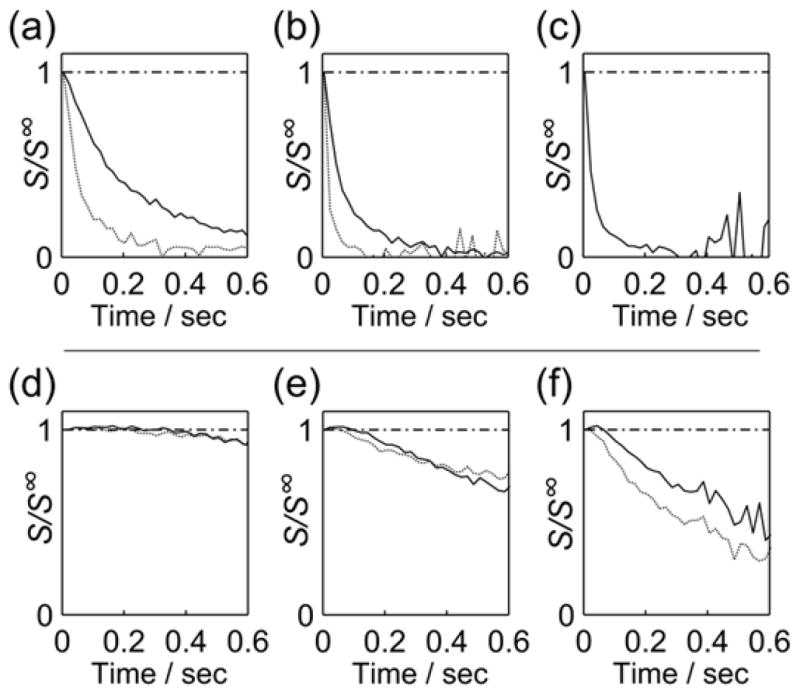
Echo signals from magnetization helices of different wavenumbers k, obtained at t_stab = 800 ms (dashed line) and t_stab = 1 s (solid line), and normalized to the intensities from a stationary sample (S^∞, t_stab = ∞). Normalized echo signals from experiments performed with the gas driven injector are shown for a) k = 10.6 cm⁻¹, b) k = 31.4 cm⁻¹ and c) k = 62.7 cm⁻¹. The dashed line in (c) is not shown, since the echoes at 800 ms were nearly undetectable. Data from the liquid driven injection is shown for d) k = 10.6 cm⁻¹, e) k = 31.4 cm⁻¹ and f) k = 62.7 cm⁻¹. A dash-dotted line at S/S^∞ = 1 is drawn as a reference in all panels.

Figure 5.

a) Schematic of the liquid driven injector. Hyperpolarized sample and non-hyperpolarized reactants can be loaded into two sample loops. Different type and size of tubing is designated by c (copper, 1/8″ OD), p1 & p2 (PEEK, 0.02″ ID; 0.062″ OD), p3 (PEEK, 0.02″ ID; 0.03″ OD), p4 & p5 (PEEK, 0.03″ ID; 0.062″ OD). b) Status of syringe pumps and two-position valves (V1 & V2) during the experiment. A solid bar indicates that the valve is in the loading position (L), and a hollow bar indicates the injection position (I). Time intervals (t_load, t_inj, t_mix, t_stab) are on the order of hundred ms (see contents Experimental Section). c) Schematic of the gas driven injector. The N₂ gas with pressure of P_f is used to inject the HP sample against a backward pressure of P_b into a 5 mm NMR tube for NMR measurements. d) The status of valves at each point in the experiment, including on/off valves (S1 & S2), a 2-position valve (V3) and a three-way valve (T). The functions of these valves and injection parameters (pressure, time intervals, etc.) are described in the text.

For a quantitative analysis, the apparent diffusion coefficient (D′) can be derived by fitting these data to Equation 4. The resulting coefficients (D′) are shown as a function of t_stab, for the gas driven injection in Figure 4a and for the liquid driven injection in Figure 4b. In all cases, the numerical value for D′ immediately following injection is several orders of magnitude larger than the self-diffusion coefficient, due to the presence of sample motions. It is apparent that the value obtained depends on the wavenumber k of the encoded magnetization helix that is analyzed. The reason for this dependence likely is that the fluid motion giving rise to these values in reality is not of diffusive nature. Therefore, the actual value of the coefficient D′ may be of lesser importance than the general trends observed. In order to facilitate the comparison of the situation in the gas and liquid driven injection, average values calculated from all observed echoes are shown in Figure 4c. Here, it is clear that the fluid motions in the liquid driven injection are much smaller at short t_stab. For example, the same average D′ = 2.3×10⁻⁸ m²s⁻¹, corresponding to 10 times the self-diffusion coefficient of water, is reached after a stabilization time of ~0.46 s in the liquid driven injection, but only after ~1.3 s in the gas driven injection under the conditions used here. Further, in the case of liquid injection, the average D′ after 0.8 s falls below 1.5x the diffusion constant of a stationary sample, while it is still > 54 times larger at the same time point in the gas driven injection.

Figure 4.

a) Apparent diffusion coefficients measured from HP samples injected using gas at various stabilization times. Data from echoes with k = 10.6 cm⁻¹, k = 31.4 cm⁻¹ and k = 62.7 cm⁻¹ is indicated by ◇, ○ and □. b) Counterpart to the data in (a), but using liquid driven injection. c) Average of the diffusion coefficients taken over all wavenumbers, obtained from HP sample injected using gas (○) and liquid (■). The horizontal dotted line indicates the self-diffusion coefficient of H₂O at 298 K.

Lower fluid motions after the liquid driven injection are advantageous for the use of experiments based on PFGs in combination with D-DNP. Experiments that employ gradient refocusing of coherences in general are prone to signal loss due to sample motions, by the same mechanism that gives rise to echo attenuation in the data shown here. Due to the single-scan nature of D-DNP, phase cycling cannot easily be applied in these experiments. The use of PFGs is of particular interest for the purpose of coherence selection,^[25] as well as for experiments that are based on spatial encoding of coherences.^[19] In all of these cases, the use of liquid driven injection as described and characterized here may be favorable. Further, the pressure and flow rate in the liquid driven injection are less variable, i.e. do not need to be optimized for different types of experiments. Finally, the use of a liquid as a driving force improves the precision of fluid handling, and reduces the propensity for introducing gas bubbles into the sample.

Conclusion

In summary, an implementation of a sample injector for D-DNP has been described, where the driving force for injection is provided by a high-pressure liquid. Two benchmarks for performance – the injection time and the linewidth in the resulting NMR spectra – are similar to those in typically employed gas driven injection devices. A characterization of residual fluid motions that persist at the time of the NMR measurement indicates that the sample stabilizes rapidly when using liquid driven injection. The absence of significant fluid motions is in particular desirable when adapting modern, pulsed field gradient based NMR experiments to D-DNP, which may otherwise be prone to signal attenuation.

Experimental Section

Sample Injection Setup

For liquid driven injection, two high-pressure, high flow rate pumps (1000D and 500D, Teledyne Isco, Lincoln, NE) are coupled to two high-pressure two-position valves (8 port, 1/8″ tubing diameter, 1.3 mm bore, titanium body, max. pressure 34.5 MPa, PN: DL8UWTI, VICI Valco Instruments, Houston, TX). In the configuration shown (Figure 5a), the syringe pumps have two different volumes, but depending on injection volume and pressure requirements could be replaced with two identical pumps of either type. A Y-mixer is included, such that a non-hyperpolarized solution can be admixed to the DNP polarized sample before entering the flow cell (modified CryoFIT^™, Bruker Biospin, Billerica, MA) for the NMR measurement. The routing of tubing between the DNP polarizer, valves and the NMR instrument is designed for automatically loading HP sample from the polarizer into loop L1, and manually loading the second sample component into loop L2 using a syringe. All tubing in the setup is made of rigid materials in order to avoid expansion. A large increase in the internal volume would lead to a pressure build-up rate insufficient for rapid sample injection. Copper tubing (1/8″ OD) connects the syringe pumps to the two-position valves. For use with corrosive liquids, copper can be replaced with stainless steel or polyether ether ketone (PEEK). The two sample loops are made of PEEK tubing (1/8″ OD, both with a total internal volume of 1 mL). The remaining connections, designated with p1–p5, use PEEK tubing of different sizes (see figure caption for details). The high pressure that can be generated by the syringe pumps might cause tubing or other components to burst, resulting in potentially unsafe conditions. To partially alleviate such hazards, relief valves (SS-4R3A, Swagelok) are located at the exit of the pump heads.

LabVIEW software (National Instruments, Austin, TX) controls the two syringe pumps and the switching of the two-position valves. The timing of each event in the sample injection process is illustrated in Figure 5b. The two pumps are set to run before the start of dissolution of the HP samples. The syringe pump with larger volume (ISCO 1000D) is started earlier because of its slower buildup of pressure. Initially, V1 and V2 are in the loading position (L), indicated by a solid bar. Once the sample loop (L1) has been filled with HP sample, an optical detector (OPB350, OPTEK Technology, Carrollton, TX) triggers the switching of V1 to the injection position (I), indicated by a hollow bar in Figure 5b and d. The fluid in pump 1 then drives the HP sample out of the loop and towards the mixer. V2 is switched to I position slightly before the HP sample arrives in the mixer to prevent part of the HP sample from flowing into the tube p2. The fluid containing HP sample then becomes mixed with the second sample component, which was pre-loaded in loop L2. As soon as the mixture arrives in the flow cell, the two pumps are stopped and both valves are switched back to the L position. In this configuration, since port 2 in V2 is blocked, a closed loop comprising the flow cell and Y-mixer is formed, which holds a constant pressure in this closed loop and causes the fluid flow to subside. After a time delay for stabilization (t_stab), the NMR measurement is performed. The start of the t_mix interval is the time point, when injection of the non-hyperpolarized reagent commences.

The gas driven sample injector, which was used for comparison, is detailed in our previous publication.^[14] Briefly, as shown in Figure 5c, before the dissolution, the NMR tube is pressurized by N₂ gas with pressure of P_b. For this purpose, the three-way valve (T) is set to connect ports b and c, and the on/off valve S1 is closed and S2 is opened. Once the sample loop L3 (Polytetrafluoroethylene, 0.0625″ ID, 1mL) is filled, the valve V3 (C22-6180, VICI Valco Instruments) is switched and N₂ gas with a pressure P_f is supplied to drive the HP sample against a backward pressure (P_b) into an NMR tube. To rapidly equilibrate the pressure in the NMR tube, the ports f and c in T are connected at the end of the injection. A delay t_stab is allowed for sample motions to subside, and the NMR acquisition follows. For experiments that require mixing, other reagents with volume 25–50 μL can be pre-loaded in the NMR tube.

NMR Experiments

To determine the optimal transfer time for sample delivery with the liquid driven injector, a 10 μL aliquot containing dimethylsulfoxide (DMSO) and D₂O (v/v 1:1) with 15 mM TEMPOL radicals (Sigma Aldrich, St. Louis, MO) was hyperpolarized in a HyperSense DNP polarizer (Oxford Instruments, Abingdon, UK) using microwaves of 94.001 GHz and 100 mW, at 1.4 K for 30 minutes. The frozen sample was dissolved using 4 mL of H₂O, which had been heated until a pressure of 10 bar was reached. The sample was then injected into a 400 MHz NMR spectrometer fitted with a triple-resonance TXI probe (Bruker Biospin, Billerica, MA) designed with a sleeve guiding the inset tubing through the probe to the flow cell. Injection was performed as described in the previous section, using H₂O as the driving fluid. For this experiment, no mixing was required, and only pump 1 was used. An array of ¹H NMR spectra was acquired by a series of radio-frequency pulses with a small tip angle (9°). The NMR experiment, including pulses and data acquisition, was triggered at the beginning of t_inj in order to be able to observe the arrival of HP sample that continuously flowed into the NMR coil. In this experiment, the time delay between excitation pulses should be long enough so that the fresh HP sample can refill the flow cell and the effect from the previous part of sample is minimized.

Once the arrival time was determined from the aforementioned experiment, the line shapes obtainable using this sample injector were characterized. A hyperpolarized aliquot containing 1.5 M benzamidine, 15 mM OX63 radicals (Oxford Instruments, Abingdon, UK) and mixture of ethylene glycol/H₂O (v/v 6:4) was dissolved with phosphate buffer (50 mM, pH=7), and injected with H₂O as described above, without admixing a non-hyperpolarized counterpart. After the stabilization time t_stab = 200 ms, a total of 16 ¹³C NMR spectra were acquired using a set of RF pulses with a tip angle of 30°.

Residual motions that persist in the sample after a rapid injection were assessed by monitoring a stimulated gradient echo train as function of time.^[15,26] For this purpose, a 10 μL aliquot of d6-DMSO/H₂O mixture (v/v 1:1) with 15 mM TEMPOL radicals was hyperpolarized on ¹H nuclei. 1 mL of 200 mM citrate buffer was manually loaded in L2 in lieu of a second sample. HP samples were injected either by the liquid driven or the gas driven injectors. In the measurements using the liquid driven injector, pumps 1 and 2 were set to nominal flow rates of 130 and 150 mL/min, and t_inj and t_mix were set to 330 ms and 420 ms. These parameters were determined by monitoring the color change of a pH indicator upon pH-jump (see Supporting Information), to ensure that mixing occurred. The mixing ratio of hyperpolarized sample with non-hyperpolarized sample was 4:1 v/v, which was determined by NMR and is reproducible. In the experiments using the gas driven injector, parameters were P_f = 1.79 MPa, P_b = 1.03 MPa, t_inj = 310 ms and h = 33 mm. A sample of 30 μL of 200 mM citrate buffer was pre-loaded in the NMR tube to mimic an experiment involving mixing. In both cases, the t_load was measured to be ~930 ms.

The pulse sequence for generating and measuring the gradient echoes is shown in Figure S2 (see Supporting Information). A superposition of magnetization helices was first created by applying N encoding pulses (with a tip angle α = 13° and pulse length=1 μs, N=16), separated by δ = 700 μs over a continuous field gradient G_z = 0.035 T/m. After a delay δ_d = 10 μs, a 90° pulse stored a projection of the resulting spatial encoding of magnetization longitudinally, in order to minimize signal loss through T₂ relaxation during the subsequent diffusion time. The time interval between each encoding pulse and the 90° storage pulse was t_n = nδ + δ_d. The index n equals to N for the first pulse, and to 1 for the last pulse. Crushing gradients (G_x = 0.056 T/m, G_y = 0.053 T/m) were applied to remove the unwanted transverse magnetization. After a diffusion time τ₁ = 5 ms, a series of RF pulses (with a flip angle β = 13° and pulse length of 2 μs) was used to create stimulated gradient echoes. The same readout procedure was repeated, until signal-to-noise ratio of echo signals deteriorated due to T₁ relaxation and the effect of pulses. The time points for each subsequent readout were τ_m = τ₁ + (m − 1) × Δτ, for m = 1, 2, .., M, with Δτ = 50 ms and M = 32. The G_z gradient described above was enabled throughout the entire experiment.

Data Analysis

The obtained stimulated echo signals were represented as an M × N matrix. The signal intensity depends on the sample displacement during the diffusion time, the effect of applying RF pulses, and the inherent spin relaxation. This dependence is shown as A^d, A^p and A^r in Equations 1–3, respectively.^[15]

$$A^d(m,n)=exp\left(-D·{(\gamma G_z{t}_n)}^2\left({\tau }_m+\frac{2t_n}{3}\right)\right)$$ (1)

$$A^p(m,n)=sin(\beta )·{cos}^{m-1}(\beta )·sin(\alpha )·{cos}^{N-n}(\alpha )·{cos}^{2(n-1)}(\alpha /2)$$ (2)

$$A^r(m,n)=exp\left(-\frac{2t_n}{T_2}\right)·exp\left(-\frac{{\tau }_m}{T_1}\right)$$ (3)

The diffusion coefficient was determined by fitting the calculated function (Equation 4) to the obtained signal matrix S (m, n), either using m or n as an independent variable with D and S⁰ as fit parameters. S⁰ is the signal amplitude of the echo in an ideal case, where the magnetization is completely refocused and no spin relaxation is present.

$$S(m,n)=S_0·A^d·A^p·A^r$$ (4)

Spin relaxation times and the G_z gradient strength, knowledge of which is required for the fitting, were determined in separate experiments, respectively, an inversion-recovery measurement and a measurement of 1D images of a phantom sample using a pulsed field gradient spin echo sequence.^[27]

References

- 1.Meier S, Jensen PR, Karlsson M, Lerche MH. Sensors. 2014;14:1576–1597. doi: 10.3390/s140101576. [DOI] [PMC free article] [PubMed] [Google Scholar]
- 2.Lee JH, Okuno Y, Cavagnero S. J Magn Res. 2014;241:18–31. doi: 10.1016/j.jmr.2014.01.005. [DOI] [PMC free article] [PubMed] [Google Scholar]
- 3.Ardenkjær-Larsen JH, Fridlund B, Gram A, Hansson G, Hansson L, Lerche MH, Servin R, Thaning M, Golman K. Proc Natl Acad Sci U S A. 2003;100:10158–10163. doi: 10.1073/pnas.1733835100. [DOI] [PMC free article] [PubMed] [Google Scholar]
- 4.Bornet A, Melzi R, Perez Linde AJ, Hautle P, Brandt B, Jannin S, Bodenhausen G. J Phys Chem Lett. 2012;4:111–114. doi: 10.1021/jz301781t. [DOI] [PubMed] [Google Scholar]
- 5.Köckenberger W. eMagRes. John Wiley & Sons; 2014. Dissolution Dynamic Nuclear Polarization; pp. 161–170. [Google Scholar]
- 6.Koptyug IV. Mendeleev Commun. 2013;23:299–312. [Google Scholar]
- 7.Keshari KR, Wilson DM. Chem Soc Rev. 2014;43:1627–1659. doi: 10.1039/c3cs60124b. [DOI] [PMC free article] [PubMed] [Google Scholar]
- 8.Bowen S, Hilty C. Angew Chem Int Ed. 2008;47:5235–5237. doi: 10.1002/anie.200801492. [DOI] [PubMed] [Google Scholar]
- 9.Miclet E, Abergel D, Bornet A, Milani J, Jannin S, Bodenhausen G. J Phys Chem Lett. 2014;5:3290–3295. doi: 10.1021/jz501411d. [DOI] [PubMed] [Google Scholar]
- 10.Cheng T, Mishkovsky M, Bastiaansen JAM, Ouari O, Hautle P, Tordo P, Brandt B, Comment A. NMR Biomed. 2013:1582–1588. doi: 10.1002/nbm.2993. [DOI] [PubMed] [Google Scholar]
- 11.Reynolds S, Bucur A, Port M, Alizadeh T, Kazan SM, Tozer GM, Paley MNJ. J Magn Reson. 2014;239:1–8. doi: 10.1016/j.jmr.2013.10.024. [DOI] [PMC free article] [PubMed] [Google Scholar]
- 12.Hu S, Larson PEZ, Vancriekinge M, Leach AM, Park I, Leon C, Zhou J, Shin PJ, Reed G, Keselman P, et al. Magn Reson Imaging. 2013;31:490–496. doi: 10.1016/j.mri.2012.09.002. [DOI] [PMC free article] [PubMed] [Google Scholar]
- 13.Ardenkjær-Larsen JH, Leach AM, Clarke N, Urbahn J, Anderson D, Skloss TW. NMR Biomed. 2011;24:927–932. doi: 10.1002/nbm.1682. [DOI] [PubMed] [Google Scholar]
- 14.Bowen S, Hilty C. Phys Chem Chem Phys. 2010;12:5766–5770. doi: 10.1039/c002316g. [DOI] [PubMed] [Google Scholar]
- 15.Granwehr J, Panek R, Leggett J, Köckenberger W. J Chem Phys. 2010;132:244507–244513. doi: 10.1063/1.3446804. [DOI] [PubMed] [Google Scholar]
- 16.Lee Y, Zeng H, Ruedisser S, Gossert AD, Hilty C. J Am Chem Soc. 2012;134:17448–17451. doi: 10.1021/ja308437h. [DOI] [PubMed] [Google Scholar]
- 17.Chen HY, Ragavan M, Hilty C. Angew Chem Int Ed. 2013;52:9192–9195. doi: 10.1002/anie.201301851. [DOI] [PubMed] [Google Scholar]
- 18.Ludwig C, Marin-Montesinos I, Saunders MG, Emwas AH, Pikramenou Z, Hammond SP, Günther UL. Phys Chem Chem Phys. 2010;12:5868–5871. doi: 10.1039/c002700f. [DOI] [PubMed] [Google Scholar]
- 19.Donovan KJ, Frydman L. J Magn Reson. 2012;225:115–119. doi: 10.1016/j.jmr.2012.10.006. [DOI] [PMC free article] [PubMed] [Google Scholar]
- 20.Bowen S, Zeng H, Hilty C. Anal Chem. 2008;80:5794–5798. doi: 10.1021/ac8004567. [DOI] [PubMed] [Google Scholar]
- 21.Frydman L, Blazina D. Nat Phys. 2007;3:415–419. [Google Scholar]
- 22.Leggett J, Hunter R, Granwehr J, Panek R, Perez-Linde AJ, Horsewill AJ, McMaster J, Smith G, Köckenberger W. Phys Chem Chem Phys. 2010;12:5883–5892. doi: 10.1039/c002566f. [DOI] [PubMed] [Google Scholar]
- 23.Chen HY, Hilty C. Anal Chem. 2013;85:7385–7390. doi: 10.1021/ac401293n. [DOI] [PubMed] [Google Scholar]
- 24.Shrot Y, Frydman L. J Chem Phys. 2008;128:164513(1)–164513(15). doi: 10.1063/1.2890969. [DOI] [PMC free article] [PubMed] [Google Scholar]
- 25.Zhang G, Schilling F, Glaser SJ, Hilty C. Anal Chem. 2013;85:2875–2881. doi: 10.1021/ac303313s. [DOI] [PubMed] [Google Scholar]
- 26.Peled S, Tseng CH, Sodickson AA, Mair RW, Walsworth RL, Cory DG. J Magn Reson. 1999;140:320–324. doi: 10.1006/jmre.1999.1850. [DOI] [PMC free article] [PubMed] [Google Scholar]
- 27.Callaghan P. Translational Dynamics and Magnetic Resonance: Principles of Pulsed Gradient Spin Echo NMR. Oxford University Press; 2011. [Google Scholar]
Associated Data
This section collects any data citations, data availability statements, or supplementary materials included in this article.