

Abstract
Motivation: Markov networks are undirected graphical models that are widely used to infer relations between genes from experimental data. Their state-of-the-art inference procedures assume the data arise from a Gaussian distribution. High-throughput omics data, such as that from next generation sequencing, often violates this assumption. Furthermore, when collected data arise from multiple related but otherwise nonidentical distributions, their underlying networks are likely to have common features. New principled statistical approaches are needed that can deal with different data distributions and jointly consider collections of datasets.
Results: We present FuseNet, a Markov network formulation that infers networks from a collection of nonidentically distributed datasets. Our approach is computationally efficient and general: given any number of distributions from an exponential family, FuseNet represents model parameters through shared latent factors that define neighborhoods of network nodes. In a simulation study, we demonstrate good predictive performance of FuseNet in comparison to several popular graphical models. We show its effectiveness in an application to breast cancer RNA-sequencing and somatic mutation data, a novel application of graphical models. Fusion of datasets offers substantial gains relative to inference of separate networks for each dataset. Our results demonstrate that network inference methods for non-Gaussian data can help in accurate modeling of the data generated by emergent high-throughput technologies.
Availability and implementation: Source code is at https://github.com/marinkaz/fusenet.
Contact: blaz.zupan@fri.uni-lj.si
Supplementary information: Supplementary information is available at Bioinformatics online.
1 Introduction
Undirected graphical models or Markov networks are a popular class of statistical tools for probabilistic description of complex associations in high-dimensional data (cf. Rue and Held, 2005). Biological processes in a cell involve complex interactions between genes and it is important to understand, which genes conditionally depend on each other. These dependencies can be inferred from the experimental data and represented in a gene network. As a popular approach to network modeling, Markov networks are particularly appealing because they focus on finding such conditional dependence relationships. Intuitively, the existence of a link between genes A and B in a Markov network indicates that the behavior of gene A is still predictive of gene B given all available measurements about gene A and its immediate neighbors in a network. Hence, Markov networks can help us to find a rich set of direct dependencies between genes that are stronger than gene correlations (Allen and Liu, 2013).
Markov networks have been well studied in bioinformatics and numerous applications are concerned with inferring the network structure primarily from microarray and next generation sequencing gene expression data (Kotera et al., 2012; Gallopin et al., 2013; Segal et al., 2003). They are complementary but not superior to other gene network inference approaches (Marbach et al., 2012). However, the increasing variety of data generating technologies and heterogeneity of resulting data draw attention to two challenges in the context of Markov network inference: inference from non-Gaussian distributed data, and simultaneous inference from many datasets.
In bioinformatics, many datasets are high dimensional, contain a limited number of samples with a large number of zeros, and come from skewed distributions. Most existing methods assume that data follow a Gaussian distribution. While this assumption holds for typical log ratio expression values from microarray data, it is violated for measurements obtained from sequencing technologies. For example, gene expression levels from RNA-sequencing count how many times a transcript maps to a specific genomic location (Wang et al., 2009) and as such these data are not Gaussian (Allen and Liu, 2013). The Gaussian assumption is also violated for categorical datasets, such as data on mutation types and copy number variation data (Hudson et al., 2010). While it would be possible to design a network inference for each specific data type, we could benefit from a procedure that can treat a wide class of distributions and can jointly consider all available data during network inference (Žitnik and Zupan, 2015).
We have developed a novel approach, called FuseNet, for inference of undirected networks from a number of high-dimensional datasets (Fig. 1). Our approach builds upon recent theoretical results about Markov networks (Yang et al., 2012, 2013) and, unlike the previous works in Markov modeling, can be applied to settings where data arise from multiple related but otherwise nonidentical distributions. To achieve this level of modeling flexibility, we represent model parameters with latent factors. FuseNet implements data fusion through sharing of latent factors that are common to all datasets and distributions, and handles data diversity through inference of factors specific to a particular dataset.
Fig. 1.

An overview of FuseNet in a toy application to network inference. FuseNet’s input is a collection of datasets that can follow different exponential family distributions. The example from the figure uses two datasets: (a) gene expressions from next-generation sequencing follow the Poisson distribution, and (b) somatic mutation data follow the multinomial distribution. (c) FuseNet infers a network by collectively modeling dependencies between any two genes conditioned on the rest of the genes. The absence of an edge between s2 and s3 (dotted line in grey) implies that s2 acts independently of s3 given s1 and s4, the neighbors of s2. The symbol stands for conditional independence. Genes s1 and s2 are linked because data profiles of s2 in (a, b) are still predictive of the profile values of s1 given s4, the neighbor of s2. (d) Shown are FuseNet-inferred coefficients that relate s2 to all other genes. Nonzero values indicate gene dependency. In the resulting network, gene s2 has two neighbors, s1 and s4
In simulation studies, FuseNet recovers the true networks underlying the observed data more accurately than several alternative approaches. The improved performance demonstrates that FuseNet can find conditional dependencies between genes that could not be reconstructed with Gaussian-based approaches. In a case study with breast cancer RNA-sequencing expression values and somatic mutation data, we demonstrate the benefits of joint network inference from multiple related datasets. The networks inferred collectively from both types of data show greater functional enrichment than networks learned from any data type alone.
2 Related work
The most straightforward approach to network inference is a similarity-based approach, which assumes that functionally related genes are likely to share high similarity with respect to a given dataset. A well-known network obtained with this approach is the S. cerevisiae genetic interaction network by Costanzo et al. (2010). Whenever the similarity value between two genes is above a threshold they are linked by an edge, which is referred to as a direct network inference approach (Kotera et al., 2012). In contrast to direct network inference, model-based network inference via graphical models focuses on local dependencies between genes, where each gene is directly affected by a relatively small number of genes. Edges estimated by a graphical model can be related to causal inference (Pearl and Verma, 1991).
The problem of learning a network structure associated with an undirected graphical model has seen a wide range of applications ranging from social networks and image and speech processing (Metzler and Croft, 2005; Wang et al., 2013) to genomics. Applications in bioinformatics include estimation of molecular pathways from protein interaction and gene expression data (Segal et al., 2003; Stingo and Vannucci, 2011), reconstruction of gene regulatory networks from microarray data (Marbach et al., 2012), inference of a cancer signaling network from proteomic data (Mukherjee and Speed, 2008) and reconstruction of genetic interaction networks from integrated experimental data (Isci et al., 2014). Methods applied to these problems and many other recent gene network inference algorithms (Anjum et al., 2009; Friedman et al., 2008; Meinshausen and Bühlmann, 2006; Ravikumar et al., 2010; Schäfer and Strimmer, 2005) estimate Gaussian or binary Markov networks, i.e. they assume that data follow an approximately Gaussian distribution.
Although non-Gaussian data are becoming increasingly common in biology, until now, very few network inference algorithms have been proposed for their treatment. When dealing with non-Gaussian data, some authors simply use methods that are based on a Gaussian assumption (Cai et al., 2012). We show in experiments that this decision may result in poor predictive performance. Recently, various extensions of Gaussian Markov networks have been proposed that first Gaussianize the data, using for example a copula transform (Liu et al., 2009, 2012; Murray et al., 2013) or a log transform, and then apply algorithms that rely on an assumption of normality. While these approaches perform better than naïve application of Gaussian-based methods to untransformed data, they are ill-suited to data generated by next generation sequencing technologies (Allen and Liu, 2013). A handful of recent algorithms (Allen and Liu, 2013; Gallopin et al., 2013) have considered Markov networks for non-Gaussian data, using for example the Poisson distribution for RNA-sequencing read counts. In contrast to our FuseNet, these methods cannot integrate datasets across different data types, thereby limiting their ability to fuse information from many datasets.
Our work presented here is similar in spirit to our recently developed methodology for data fusion via collective matrix factorization (Žitnik and Zupan, 2015). The methodology therein can jointly model any number of datasets that can be represented with matrices. Unlike existing data integration approaches, it does not require transforming data into a common data space (e.g. a gene space). We applied this methodology to mining disease-disease associations (Žitnik et al., 2013), predicting drug toxicity (Žitnik and Zupan, 2014) and gene functions (Žitnik and Zupan, 2015) and observed substantial gains in predictive accuracy. While both our work here and in Žitnik and Zupan (2015) rely on latent factor models, they are substantially different from one another. First, FuseNet builds on the Markov network theory, whereas previously we considered matrix decomposition. Second, FuseNet is a probabilistic model that explicitly considers various data distributions, and third, FuseNet is a network inference approach, whereas our previous works focused on matrix completion.
3 Methods
FuseNet takes as its input a collection of datasets where each dataset consists of a set of gene profiles (Fig. 1). Gene profiles can be heterogeneous and belong to different data types, e.g. data can be continuous, discrete or categorical. For example, measurements from RNA-sequencing represent the numbers of fragments that were mapped to a specific genomic location (Wang et al., 2009). The RNA-sequencing expression values are then non-negative and integer valued and, hence, are not approximately Gaussian, but rather follow the Poisson or negative binomial distribution. This is in contrast to copy number variation data and mutation data, i.e. single-base substitutions, short indels, or multiple base substitutions, that might be modeled better with multinomial or categorical distributions. On the other end of spectrum are microarray gene expression data, which are approximately Gaussian distributed.
The crucial feature of FuseNet is the representation of model parameters via latent factors. This feature, together with the sharing of latent factors between datasets, allows us to infer a network by simultaneously considering many datasets that each can arise from a different exponential family distribution (Section 3.7).
We exemplify FuseNet by deriving Markov network models for two distributions from an exponential family, the Poisson distribution (Section 3.3) and the multinomial distribution (Section 3.5). Since the exponential family includes not only Gaussian but also binomial, multinomial, Poisson, gamma distributions and others, FuseNet can achieve great flexibility in estimating gene networks from diverse data (Section 3.6) and also comes with an efficient algorithm for network structure estimation (Section 3.8).
Our work provides two novel contributions over current approaches to gene network inference discussed in Related work:
FuseNet simultaneously infers networks from datasets that may be generated by nonidentical distributions, and
FuseNet estimates large-scale genomic networks from increasingly common non-Gaussian distributed data.
3.1 Preliminaries
3.1.1 Markov networks
A Markov network specifies conditional dependence relationships between genes. In particular, if there is no edge between genes s and t then this implies that the behavior of s is independent of t given the set of immediate neighbors of s. From this local property (Murphy, 2012), one can easily see that two genes (nodes) are conditionally independent given the rest of the genes iff there is no direct edge between them. The conditional independence (Markov) properties permit a rich set of dependencies among the nodes and hence, the connectivity of a Markov network can reveal complex relationships between its nodes (Allen and Liu, 2013; Jalali et al., 2011).
3.1.2 Exponential family
The probability distributions that we study in this article are specific examples of a broad class of distributions called the exponential family (Duda and Hart, 1973). Members of the exponential family have many important properties in common. Given parameters θ, the exponential family of distributions over X is defined to be the set of distributions of the form:
| (1) |
where B(X) are sufficient statistics, C(X) is a base measure and is a log-normalization constant (Murphy, 2012). The exponential family includes many widely used distributions, such as Bernoulli, binomial, Poisson, gamma, multinomial and Gaussian distributions.
3.1.3 Parameterization of Markov networks
Let be a random vector with Xi being a random variable. Suppose is an undirected graph with p nodes representing p variables in X, . Then the corresponding undirected graphical model is any distribution defined on X that satisfies Markov independence assumptions with respect to graph G (Murphy, 2012). By the Hammersley-Clifford theorem (Murphy, 2012), any such distribution of X decomposes according to graph G in the following way. Let be a set of maximal cliques (fully connected subgraphs) in graph G and let be “clique potential” functions. By the Hammersley-Clifford theorem, any distribution of X within the graphical model family defined by G can be represented as an exponential of a weighted sum of potential functions over the maximal cliques :
| (2) |
where are the weights of potential functions.
An important question is how one would select potential functions to obtain various multivariate extensions of univariate distributions. Recently, Yang et al. (2012) showed that if a node-conditional univariate distribution, i.e. distribution of a random variable conditioned on all other variables, belongs to an exponential family, it necessarily follows that the joint distribution of X has the form:
| (3) |
where the cliques are of size at most k, are neighbors of node s, B represent sufficient statistics and C is the base measure of the a given exponential family distribution (cf. Proposition 1 and Proposition 2 in Yang et al. (2012)). These results tell us that the joint distribution specified in Eq. (3) has the most general form under the assumption of exponential family node-conditional distributions. Hence, learning a graphical model from the data can be reduced to learning weights of distribution-specific sufficient statistics.
3.2 Problem definition
Suppose we are given a collection of n observations, , where is a p-dimensional vector drawn i.i.d. from a specific distribution of the form in Equation (3). This distribution has parameters and is associated with a graph on p nodes. Graph G encodes Markov independence properties between the respective variables. The goal of learning the structure of G is to infer an edge set that corresponds to distribution, which generated observations in . We can express as a function of parameters and write it as:
Hence, learning the network structure reduces to the problem of estimating weights that should be as close as possible to the true but otherwise unknown parameters .
In this article, we focus largely on a special case of pairwise Markov networks, where the joint distribution has cliques of size at most two:
| (4) |
with entries if and if . Following the work of Ravikumar et al. (2010), Jalali et al. (2011) and Allen and Liu (2013), we approach the problem of Markov network structure learning via neighborhood estimation, where we obtain the global network estimate by stitching together the estimated neighborhoods of the nodes. The overall network structure is then:
| (5) |
where (s, t) denotes an edge between s and t and is the estimated neighborhood of node s.
In the remainder of this section, we formulate two pairwise Markov networks, which assume either Poisson or multinomial data distribution. These two exponential family models are taken as an example through which we specify a general scheme for network inference from multiple potentially nonidentical data distributions.
3.3 Poisson model specification
Following the work of Yang et al. (2012) and Allen and Liu (2013), we define a Poisson Markov network model by specifying a distribution where all node-conditional distributions follow a univariate Poisson distribution. Our Poisson Markov network model is then a series of locally defined models, one for every variable (node). A local model for s is given by a distribution of Xs conditioned on all other variables:
| (6) |
where denotes the rest of the variables, and and are model parameters. An r-dimensional vector is a latent factor for node s that consists of r latent components. For now, we assume that the number of latent components r is given; we will later discuss how to automatically determine r. Notice that the latent factor of node s, , represents the strength of membership of node s to r latent components and W models the interactions between all combinations of r latent components. The formulation of the Poisson conditional distribution in Equation (6) ensures that node pair-wise weights are symmetric, which is an appealing property when studying undirected graphical models. In particular, the contribution of Xt towards is the same as is the contribution of Xs towards .
We refer to our model as a model parameterized via latent factorization, since model parameters and W form a factorization of the edge weight θst, which is specified by a Markov network model in Equation (4). The importance of latent factor parameterization will be obvious later in Section 3.7 when we discuss collective network inference from many datasets.
Recall the univariate Poisson distribution is given by the mass function , where λ is the shape parameter. Our model extends the univariate Poisson in a natural and strict sense to the multivariate graphical model setting. The latter can be obtained from the univariate Poisson by setting the shape parameter to . We then write the expression in Equation (6) as:
| (7) |
Intuitively, variable Xs in Equation (7) can be viewed as the response variable in a latent factor Poisson regression in which the other variables play the role of the predictors. Variables with strong relationships with gene s will have nonzero regression coefficients, and these will be connected to node s in the inferred graph.
3.4 Optimization of the Poisson model
The node-conditional distributions specified in Equation (7) define a global distribution that factors according to the cliques of the underlying graph G that we would like to estimate. We obtain edge set by stitching node neighborhoods as prescribed by Equation (5), where we define the neighborhood of node s as . This means that edge (s, t) is included in the network if the estimated product of respective latent factors of variables Xs and Xt is nonzero.
To estimate edge set , we have to determine the node neighborhoods of all nodes in V. To achieve this goal, we solve a sparsity constrained conditional maximum likelihood estimation problem:
| (8) |
Here, U is a matrix with node latent factors placed in the columns, .
Equation (8) consists of two parts, which we discuss next. Terms involving Reg represent the elastic net penalties (Zou and Hastie, 2005). The penalty is defined for U as , where is a regularization parameter controlling the amount of sparsity in the node neighborhood. The definition of the penalty term for W is analogous. Notice that the norm is the sum of 2-norms of the columns, , and the norm is the sum of 1-norms of the columns, . Since latent factors are affected by the strength of regularization, the choice of parameter λ is important. Procedure for selection of λ is described in Supplementary Section 1.
The crucial part of Equation (8) is, however, the sum of the node-wise Poisson likelihood functions. Given node s and n realizations of the associated random variable Xs, the Poisson likelihood function follows directly from Equation (7) and can be written as:
| (9) |
where is the i-th realization of Xs in data denotes the i-th realization of the rest of the variables , and U and W are matrix unknowns. Notice that node-wise terms are ignored here for simplicity.
3.5 Multinomial model specification and optimization
We now develop a multinomial Markov network model that relies on latent factor parameterization of the model parameters and follows the same paradigm as our Poisson model described in the previous section. The multinomial model presented here is a natural extension of the multinomial graphical model described by Jalali et al. (2011).
We start with the neighborhood recovery of one fixed node s and then combine the neighborhood sets across nodes to estimate the network. The multinomial model assumes that each variable Xi from a random vector X follows a multinomial distribution with potentially different parameters. This means that Xi can take any value from a small discrete set of cardinality m. Probabilities of different values are not independent so that, given any m – 1 of the probabilities, the probability of the remaining value is fixed. It is convenient to express the distribution in terms of only m – 1 values, thereby leaving m – 1 probability parameters that need to be estimated.
The distribution of Xs conditioned on other variables is given by:
| (10) |
for all . Here, θsj represents a node-wise term that models the probability of variable Xs taking value j. The other model parameter is , which models dependency between variable Xs and variable Xt when they take values j and k, respectively. We can view Equation (10) as a multiclass logistic (softmax) regression, where Xs is the response variable and indicator functions associated with other variables:
where , are the predictors.
We now proceed by writing model parameters θsj and in the form of a product of latent factors. We gather node-wise terms θsj into a matrix . We factorize as . Here, and are r-dimensional latent factors and encodes interactions between latent components in the same way as is described in Section 3.3.
To estimate the latent factors and node-wise terms from the data we solve the following convex optimization program:
| (11) |
where definitions of U, W and Reg are the same is in the previous section. Here, the node-wise multinomial likelihood function for node s follows from Equation (10) and can be written as:
| (12) |
where is the i-th realization of Xs in data denotes the i-th realization of the rest of the variables , and U, Q and W are matrix unknowns. Given latent factor estimates U and W, and the estimate of node-wise terms Q, we determine the neighborhood for node s as . This means that edge (s, t) is included in the network if product does not vanish over at least one choice of categories j and k.
3.6 Other exponential family distributions
So far, we described in Section 3.3–3.5, the Poisson model and the multinomial model that are suitable for separately inferring the edge set of a Poisson or a multinomial Markov network. In this section, we would like to allude to the fact that a procedure with derivations very similar to those in the above sections can be applied to any exponential family distribution.
From Equation (1), we see that the unnormalized probability of an exponential family distribution can be expressed as an exponential of a weighted linear combination of sufficient statistics. These sufficient statistics correspond to clique potential functions (see Sec. 3.1.3). Under the assumption of joint distribution having cliques of size at most two, node-conditional distributions take the form:
where and are parameters that shall be estimated from the data.
FuseNet yields a general framework for including data from any exponential family distribution, such as Gaussian, binomial, Poisson or multinomial distributions, in its predictive model by simply expressing weights and of a given distribution as products of appropriately selected latent factors. Here, factorization of the weights is appropriate if it allows fusion of data from diverse distributions, such that factorization consists of both latent factors that are shared between different distributions and factors that are specific to a particular distribution (Žitnik and Zupan, 2015), a property that we describe in the following section.
3.7 Collective inference of a gene network
We proceed by formulating a collective network inference model, wherein a network is jointly estimated from multiple nonidentical data distributions.
Let be a set of nx observations of a random vector X, where each p-dimensional vector is drawn from a distribution Px of the form of Equation (4) and let be a set of ny observations where each p-dimensional vector is drawn from distribution Py of the form of Equation (4). Importantly, distributions Px and Py are not necessarily identical in terms of their parameters or distribution type. For example, Px might denote the Poisson distribution and Py might be the multinomial distribution or they could both describe multinomial distributions that have different parameters. For simplicity of notation we provide here the formulation for the case with only two datasets, and , but notice that our analysis generalizes to any number of datasets.
In collective network inference, we solve for:
| (13) |
where regularization parameters depend on the form of data distributions. In a specific scenario in which Px and Py are the Poisson and the multinomial distributions, respectively, we set . We specify the regularization according to the Poisson model in Equation (8) and the multinomial model in Equation (11) as:
where is the elastic net penalty defined in Section 3.3. The estimated neighborhood of node s, which corresponds to a random variable , are then nodes whose behavior depends on behavior of s according to any of considered data distributions, . In our specific scenario, parameters and would be given by and .
It is important to notice the coupling of the parameters in FuseNet through which data fusion is achieved (Žitnik and Zupan, 2015). As is evident from Equation (13), the latent factor of node s, , participates both in terms associated with Px and terms related to Py. Hence, a good estimate of should simultaneously minimize both and , but should do so in a way that statistics internal to both data distributions are considered. To account for the fact that datasets may disagree and differ in how accurately they capture biological signals, FuseNet has parameters that are specific to every distribution. In particular, we allow that interactions between latent components in are different from those in and hence, the model has one latent matrix W for each distribution. An additional parameter Q captures the characteristics of a particular exponential family distribution, e.g., the bias associated with m categories in the multinomial distribution.
3.8 Learning the models in practice
Now that we defined the FuseNet model, we explain how to solve related optimization problems. Notice that the exact optimization problem one needs to solve depends on a particular data setting, i.e. a particular combination of considered exponential family distributions.
There has been a strong line of work on developing fast algorithms to solve sparse regression problems that are similar to Equations (8) and (11) including the work by Krishnapuram et al. (2005), Meier et al. (2008), Jalali et al. (2011) and Allen and Liu (2013). Existing algorithms for undirected graphical model selection assume that model parameters are independent of each other. This, however, is not true in FuseNet due to reasons discussed in Section 3.7 that are important to achieve data fusion. Consequently, this also means that we cannot use off-the-shelf optimization solvers.
We propose to fit our FuseNet by computing cyclical coordinate descent along the path of regularization parameter λ (see Supplementary Section 1). Parameters of FuseNet inference algorithm, i.e. regularization and latent dimensionality, are selected in data-dependent way via stability selection. Interested reader is referred to Supplementary Section 1.
4 Experimental setup
We compare the performance of FuseNet to several state-of-the-art Markov network models in estimating the true underlying network structure.
4.1 Performance evaluation
The success of network recovery is evaluated by comparison to the gold standard networks, when they are available, and by functional enrichment of the inferred networks.
4.1.1 Assessing the accuracy of network recovery
Simulated data come with complete and unambiguous true underlying networks, hence we can assess the performance of the algorithms as follows. We report receiver operator curves (ROC) computed by varying the regularization parameter λ, precision recall (PR) curves, and true and false positive rates for fixed λ as estimated via stability selection. The true positive rate is estimated as proportion of the edges found by a network inference algorithm that are also in the true network. The false positive rate represents proportion of the edges in the inferred network that are not present in the true network. An algorithm with a perfect performance achieves an area under the ROC curve of 1, precision of 1 and recall of 1, a true positive rate of 1 and a false positive rate of 0.
4.1.2 Quantifying the functional content of inferred networks
We employ two approaches to evaluate the ‘functional correctness’ of the networks inferred from cancer data. First, we use SANTA (Cornish and Markowetz, 2014) to quantify the strength of association between sets of functionally related genes from the Gene Ontology (GO) (Ashburner et al., 2000) and the inferred network. Second, we overlay the inferred network with gene information from the GO and for every GO term assess how community-like a subnetwork of genes that belong to a particular GO term is. Communities are sets of genes with many connections between the members and few connections to the rest of the network. Four different structural notions of network communities exist in networks and we report the values of their representative scoring functions (Yang and Leskovec, 2012). We refer the reader to Supplementary Section 4 for mathematical details.
4.2 Considered gene network inference algorithms
In the experiments, we consider the Poisson FuseNet (Section 3.3), the multinomial FuseNet (Section 3.5) and FuseNet with fusion of Poisson and multinomial data distributions (Section 3.7). We compare our models to the Graphical Lasso (GLASSO) (Friedman et al., 2007), which is a widely used Markov network model based on a Gaussian assumption. To see how FuseNet relates to techniques that perform data preprocessing, we consider the GLASSO after applying a log transform to the data plus one (e.g. cf. Gallopin et al., 2013) and the GLASSO with the nonparanormal Gaussian copula transformation (NPN-Copula) (Liu et al., 2009). We also compare FuseNet with two Markov network models that are designed for non-Gaussian distributed data: the Local Poisson Graphical Model (LPGM) (Allen and Liu, 2013), and the Multinomial Markov Network Model (Mult-GM) (Jalali et al., 2011). The crucial parameter of these methods is degree of regularization, which controls sparsity of the networks. We select the value for regularization via stability selection (see Supplementary Section 1).
5 Data
Network inference algorithms are evaluated based on simulated data and large-scale cancer genomic datasets.
5.1 Multivariate data simulation
Four network structures are simulated: (i) the Erdős Rényi random network, where an edge between each pair of nodes is set with equal probability and independently of other edges; (ii) a hub network, where each node is connected to one of three hub nodes; (iii) a scale-free network, in which node degree distribution follows a power-law; and (iv) a small-world network, in which most nodes are not neighbors of each other but most nodes can be reached from every other by a small number of hops. We refer the reader to Supplementary Section 2 for detailed description of the procedures used for data simulation.
5.2 Cancer genomic data
We apply network inference algorithms to two examples of non-Gaussian high-throughput genomic data to learn (i) an mRNA expression network, (ii) a somatic mutation network and (iii) a collectively inferred gene network based on both data types.
We download breast cancer (BRCA-US) gene expression data measured by next generation sequencing and breast cancer (BRCA-US) simple somatic mutation data from the International Cancer Genome Consortium (ICGC) (Hudson et al., 2010) portal (release 17). We follow the steps in Allen and Liu (2013) and process RNA-sequencing data to be approximately Poisson. Data preprocessing, whose detailed steps are described in Supplementary Section 3, results in a matrix with rows as the subjects () and columns as genes (). These genes form the nodes of our Poisson breast cancer mRNA network.
Breast cancer simple somatic mutation data include single base substitutions, multiple base substitutions and short indels. Mutation data are converted into a matrix with rows as subjects () and columns as genes containing mutations or variations (500 genes). Each matrix entry is categorized into one of three groups based on the type of mutation: no mutation, single base substitution, insertion/deletion of < 200 base pairs.
For the collectively inferred network, we consider both gene expression profiles and somatic mutation data provided by the ICGC assuming the Poisson model for the RNA-seq data and the multinomial model for the mutation data. We refer the reader to Supplementary Section 3 for more details.
6 Results and discussion
6.1 Network recovery with simulated data
In every simulation, we generated a dataset of observations based on a simulated network and then applied different network inference algorithms to determine whether the algorithms successfully recovered complex relationships between data variables.
We simulated four network types, which are known to resemble the structure of real biological networks (Allen and Liu, 2013; Costanzo et al., 2010). We report receiver operator curves computed by varying the regularization parameter λ in Figure 3 and Supplementary Figure S4, boxplots of true and false positive rates for fixed λ as determined by stability selection in Figure 3, Supplementary Figures S2 and S4. Further, we evaluated precision and recall of the networks estimated from different data distributions in Supplementary Figures S2–S5.
Fig. 3.
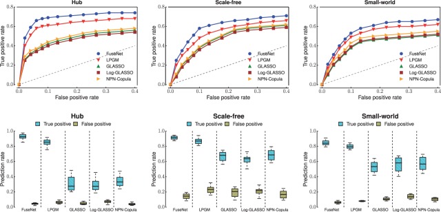
Application of gene network inference algorithms to Poisson-distributed simulated data. Simulation studies on four network types were performed: random (see Supplementary Fig. S4), hub, scale-free and small world. These graph structures appear in many real biological networks. For each graph type, we generated data with n = 200 observations with P = 100 variables (nodes) at a low (first row) and high (second row) signal-to-noise ratio (SNR). Receiver operating curves and boxplots are shown for Poisson FuseNet (proposed here), the Local Poisson Graphical Model (LPGM) (Allen and Liu, 2013), the Graphical Lasso (GLASSO) (Friedman et al., 2007), the GLASSO on log-transformed data (Log-GLASSO) (e.g. cf. Gallopin et al., 2013) and the GLASSO on data transformed through nonparanormal Gaussian copula (NPN-Copula) (Liu et al., 2009)
Experimental evidence indicates that FuseNet outperforms Gaussian-based competitors (GLASSO, Log-GLASSO and NPN-Copula) as well as existing methods that are designed specifically for the Poisson and the multinomial data (LPGM in Fig. 2 and Mult-GM in Fig. 3). The overall good performance of FuseNet is consistent across the four types of network structure and the two data distributions that we considered in experiments.
Fig. 2.
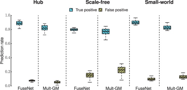
Application of gene network inference algorithms to multinomial-distributed simulated data. Simulation studies on four network types were performed: random (see Supplementary Fig. S2), hub, scale-free and small world. For each graph type, we generated n = 300 observations at a high signal-to-noise ratio (SNR) with P = 50 variables (nodes) taking values from an alphabet of size m = 3. Boxplots are shown for multinomial FuseNet (proposed here) and the multinomial graphical model (Mult-GM) (Jalali et al., 2011)
The improved statistical power of FuseNet and LPGM over methods that during network inference rely heavily on the assumption of normality is particularly impressive. Results in Figure 3 suggest that in situations where this assumption is not satisfied, we can expect reduced prediction performance if we naively apply Gaussian-based methods, (GLASSO) or if we perform insufficient data preprocessing (Log-GLASSO). However, we note that sophisticated techniques that replace Gaussian distributed data by the transformed data obtained, e.g. through a semiparametric Gaussian copula (NPN-Copula; Liu et al. (2009)), can give substantial gains in accuracy over the naive analysis. These observations are not surprising as disregarding information about data distribution can adversely affect performance of prediction models. Our results demonstrate that employing the ‘correct’ statistical model, in this case FuseNet or LPGM, can lead to more accurate network inference.
Next, we try to understand which algorithmic component of FuseNet contributes most to its good performance relative to existing algorithms for network structure learning. The primary difference between FuseNet and non-Gaussian-based methods considered here, LPGM and Mult-GM, is representation of model parameters with products of latent factors. In LPGM and similarly in Mult-GM, a prediction model is fitted locally by an algorithm, which performs a series of independent penalized regressions. This is in contrast with FuseNet, where different model parameters are not entirely independent of each other but rather rely on borrowing strength from each other via factorization. Our results on simulated data suggest that representation of model parameters through the use of latent factors is beneficial. Furthermore, latent parameterization can improve performance of network recovery beyond what is possible with models that do not use latent factors. On the downside, we note that due to coupling of model parameters, FuseNet is not trivially parallelizable, which is otherwise true for LPGM and Mult-GM.
Results shown in Figures 2 and 3 are reported for datasets with a few hundred observations (n) and a few tens of variables (p; see figure captions). We note that reported results are consistent with experiments done in various high-dimensional scenarios even when the number of variables is greater than the number of observations (p > n). Results therein reveal the same trend, namely, the overall strong performance of FuseNet in recovering true networks from non-Gaussian data.
6.2 Functional content of genomic networks
An important challenge in cancer systems biology is to uncover complex dependencies between genes implicated in cancer. Since our knowledge about genome-scale gene networks is incomplete and only a few functional modules are known for higher organisms (Rolland et al., 2014), our aim is to quantify associations between the inferred gene networks and known cellular functions and phenotypes, and to assess the significance of these associations.
6.2.1 Comparison of FuseNet variants with existing methods
To characterize how functionally informative the inferred networks are, we employ four structural definitions of network communities (Fig. 4 and Supplementary Figs S6 and S7). These represent four possible notions of association between a given GO term and the inferred network (Yang and Leskovec, 2012). The triangle participation ratio quantifies how well genes that are members of a given GO term are linked to each other in the inferred network. The cut ratio captures the abundance of external connectivity, i.e. edges between genes of a GO term and the rest of the network, whereas conductance and flake-ODF consider both internal and external network connectivity. Through these four measures we are able to estimate the overall concordance of inferred gene networks and known functional annotation of genes. For these reasons, networks that score higher on many measures should be considered more informative across a wider spectrum of cellular functions.
Fig. 4.
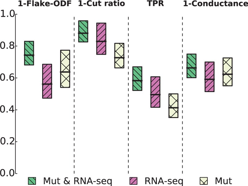
The strength of association between gene sets from the Gene Ontology (GO) and networks inferred with FuseNet. Inferred networks were overlaid with GO terms and subnetworks induced by each GO term were assessed for how well they corresponded to network communities. Four different scoring functions were used to quantify the presence of different structural notions of communities (Supplementary Section S4) that can appear in biological networks: flake-over-median-degree (flake-ODF), cut ratio, triangle participation ratio (TPR) and conductance. Considering breast cancer RNA-sequencing (RNA-seq) and somatic mutation data (Mut), these boxplots show the gains that fusion of data from different distributions (Mut & RNA-seq) can offer over network inference from any dataset alone, either RNA-seq or Mut. Poisson FuseNet was used with RNA-sequencing data, multinomial FuseNet with somatic mutation data and fully-specified FuseNet for joint consideration of RNA-sequencing and mutation data
Figure 4 shows that gene network inferred by FuseNet through fusion of breast cancer RNA-sequencing data and somatic mutation data is more concordant with functional annotation data in the GO than are networks inferred by FuseNet from either RNA-sequencing or somatic mutation data alone. We note that we used Poisson FuseNet to infer network from RNA-sequencing data, multinomial FuseNet to infer network from somatic mutation data and collective FuseNet for joint network inference from RNA-sequencing and mutation data. These results demonstrate that combining data through the use of latent factors can perform better than independent modeling of each dataset alone.
For each of the four community scoring measures in Figure 4, we compared score distributions of GO terms across three networks inferred by FuseNet using Kolmogorov-Smirnov tests. We concluded that the network inferred by FuseNet through fusion of RNA-sequencing and mutation data associates with GO significantly more strongly than the other two networks (P value < 1 × 10⁻⁵ on all four measures from Fig. 4). This experiment shows how cancer genomic data provide different levels of information about cellular machinery, highlighting that it is possible to infer a network that better explains the mechanisms of cancer by combining multiple datasets in a principled statistical way.
We further compared FuseNet to existing network inference methods on cancer data. The comparison was made only with LPGM, as this was the best performing method in our study on simulated data (Section 6.1) and in the cancer-data study of Allen and Liu (2013). Supplementary Figure S6 shows the functional content of the networks inferred from RNA-sequencing data by either Poisson FuseNet or LPGM. On a related note, Supplementary Figure S7 shows enrichment of the networks inferred from somatic mutation data by either multinomial FuseNet or Mult-GM. Notice that LPGM and Mult-GM were designed for data that are approximately Poisson distributed, such as measurements from RNA-sequencing, and multinomially distributed, such as various types of gene variations, respectively. These results demonstrate that networks inferred by FuseNet can better capture known GO annotations than networks obtained by methods such as LPGM and Mult-GM, whose prediction models do not have factorized representation. These observations are consistent across four complementary structural definitions of GO terms, where every GO term is viewed as a network community defined by its member genes.
6.2.2 Networks via breast cancer data
We employ SANTA (Cornish and Markowetz, 2014) to quantify the functional content of gene networks. SANTA extends the concept of gene set enrichment analysis to networks. We observed that GO terms indeed cluster more strongly on Poisson FuseNet’s networks than on networks inferred by GLASSO and Log-GLASSO (P value < 1 × 10⁻⁶, RNA-seq network), NPN-Copula (P value < 1 × 10⁻⁵, RNA-seq network) and LPGM (P value < 1 × 10⁻⁴, RNA-seq network). These results suggest that network edges inferred by FuseNet might represent more accurate indication of shared cellular functions than edges inferred by other considered methods. This effect was independent of the GO term size and was strongest for specific cellular functions such as ‘centrosome cycle’ (P value < 1 × 10⁻⁹), ‘cellular response to DNA damage stimulus’ (P value < 1 × 10⁻⁹), ‘apoptotic process’ (P value < 1 × 10⁻⁹) and ‘regulation of cytokinesis’ (P value < 1 × 10⁻⁸). We observed similar results when inferring networks from somatic mutation data. Gene network inferred by multinomial FuseNet was functionally richer than network inferred by Mult-GM. Here, the functional content of a network was quantified with SANTA as proportion of evaluated GO terms whose association strength with the network had P value < 1 × 10⁻⁵.
Interactions that are captured by fusing both cancer related datasets recovered many gene–gene associations that have been previously linked to increased breast cancer predisposition and metastasis. For example, FuseNet revealed a hypothesized transcriptional regulatory GATA3 module (Wang et al., 2014) consisting of fully connected GATA3, PTCH1, NFIB and PPARA. GATA3 is an important transcriptional regulator in breast cancer (Theodorou et al., 2013), and low expression levels of GATA3 are associated with a poor prognosis (Albergaria et al., 2009). It has been shown by Wang et al. (2014) that PTCH1, PPARA and NFIB exhibit epistatic interactions with GATA3, have negatively correlated expression levels with GATA3 and that GATA3 binds to gene regions near NFIB, PTCH1 and PPARA in breast epithelial tumor cell line.
Other interactions identified in our network include ATM and BRCA1, ATM and BRCA2, and CHEK2 and BRCA2, which are known gene-gene interactions whose mutations affect breast cancer susceptibility (Turnbull et al., 2012).
Another transcriptional module that was found by FuseNet consists of FLI1, JAK2 and CCND2. This module has been only recently associated with breast cancer patient outcome (Wang et al., 2014). Interestingly, FLI1 module has been captured by FuseNet when fusing RNA-sequencing and mutation data but has been missed when using FuseNet with any of the two cancer datasets in isolation, as well as by any other inference algorithm considered in this study. One possible explanation for the latter result might be observations made by Wang et al. (2014). Wang et al. examined The Cancer Genome Atlas breast cancer patient survival data and found that low expression or mutation in one or more members of the FLI1 module is associated with reduced overall survival time in all patients. The illustrative example of FLI1 module highlights an advantage of FuseNet over methods considering a single dataset during network inference.
7 Conclusion
FuseNet is an approach for automatic inference of gene networks from data arising from potentially many nonidentical distributions. It is based on the theory of Markov networks, where the inferred network edges denote a type of direct dependence that is stronger than merely correlated measurements. An appealing property of FuseNet is its ability to estimate network edges by fusing potentially many datasets. In the case studies, FuseNet’s models outperform several state-of-the-art undirected graphical models. We show that FuseNet’s high performance is attributed to the ability to model non-Gaussian distributions and fusion of data through sharing of latent representations. Our work here has broadened the class of off-the-shelf network inference algorithms for simultaneously considering a wide range of parametric distributions and has combined Markov network inference with data fusion.
Funding
This work was supported by ARRS (P2-0209, J2-5480), EU FP7 (Health-F5-2010-242038) and NIH (P01-HD39691).
Conflict of Interest: none declared.
Supplementary Material
References
- Albergaria A., et al. (2009) Expression of FOXA1 and GATA3 in breast cancer: the prognostic significance in hormone receptor-negative tumours. Breast Cancer Res. , 11, R40. [DOI] [PMC free article] [PubMed] [Google Scholar]
- Allen G.I., Liu Z. (2013) A local poisson graphical model for inferring networks from sequencing data. IEEE Trans. NanoBiosci. , 12, 189–198. [DOI] [PubMed] [Google Scholar]
- Anjum S., et al. (2009) A boosting approach to structure learning of graphs with and without prior knowledge. Bioinformatics , 25, 2929–2936. [DOI] [PubMed] [Google Scholar]
- Ashburner M., et al. (2000) Gene Ontology: tool for the unification of biology. Nat. Genet. , 25, 25–29. [DOI] [PMC free article] [PubMed] [Google Scholar]
- Cai Y., et al. (2012) Utilizing RNA-seq data for cancer network inference. In: Pal R., Ressom H. (eds), IEEE GENSIPS. IEEE, Piscataway, NJ, USA, pp. 46–49. [Google Scholar]
- Cornish A.J., Markowetz F. (2014) SANTA: quantifying the functional content of molecular networks. PLoS Comput. Biol. , 10, e1003808. [DOI] [PMC free article] [PubMed] [Google Scholar]
- Costanzo M., et al. (2010) The genetic landscape of a cell. Science , 327, 425–431. [DOI] [PMC free article] [PubMed] [Google Scholar]
- Duda R.O., Hart P.E. (1973) Pattern Classification and Scene Analysis . Wiley, New Jersey, NJ, USA. [Google Scholar]
- Friedman J., et al. (2007) Sparse inverse covariance estimation with the lasso. Biostatistics , 9, 432–441. [DOI] [PMC free article] [PubMed] [Google Scholar]
- Friedman J., et al. (2008) Sparse inverse covariance estimation with the graphical lasso. Biostatistics , 9, 432–441. [DOI] [PMC free article] [PubMed] [Google Scholar]
- Gallopin M., et al. (2013) A hierarchical Poisson log-normal model for network inference from RNA sequencing data. PLoS One , 8, e77503. [DOI] [PMC free article] [PubMed] [Google Scholar]
- Hudson T.J., et al. (2010) International network of cancer genome projects. Nature , 464, 993–998. [DOI] [PMC free article] [PubMed] [Google Scholar]
- Isci S., et al. (2014) Bayesian network prior: network analysis of biological data using external knowledge. Bioinformatics , 30, 860–867. [DOI] [PMC free article] [PubMed] [Google Scholar]
- Jalali A., et al. (2011) On learning discrete graphical models using group-sparse regularization. In: Dudík M. (ed.), AISTATS. MLR, Boston, MA, USA, pp. 378–387. [Google Scholar]
- Kotera M., et al. (2012) GENIES: gene network inference engine based on supervised analysis. Nucleic Acids Res. , 40, W162–W167. [DOI] [PMC free article] [PubMed] [Google Scholar]
- Krishnapuram B., et al. (2005) Sparse multinomial logistic regression: fast algorithms and generalization bounds. IEEE TPAMI , 27, 957–968. [DOI] [PubMed] [Google Scholar]
- Liu H., et al. (2012) High-dimensional semiparametric Gaussian copula graphical models. Ann. Stat. , 40, 2293–2326. [Google Scholar]
- Liu H., et al. (2009) The nonparanormal: Semiparametric estimation of high dimensional undirected graphs. JMLR , 10, 2295–2328. [Google Scholar]
- Marbach D., et al. (2012) Wisdom of crowds for robust gene network inference. Nat. Methods , 9, 796–804. [DOI] [PMC free article] [PubMed] [Google Scholar]
- Meier L., et al. (2008) The group lasso for logistic regression. J. R. Stat. Soc., 70, 53–71. [Google Scholar]
- Meinshausen N., Bühlmann P. (2006) High-dimensional graphs and variable selection with the lasso. Ann. Stat. , 34, 1436–1462. [Google Scholar]
- Metzler D., Croft W.B. (2005) A Markov random field model for term dependencies. In: Marchionini G., et al. (eds), ACM SIGIR. ACM, New York, NY, USA, pp. 472–479. [Google Scholar]
- Mukherjee S., Speed T.P. (2008) Network inference using informative priors. Proc. Natl. Acad. Sci. USA , 105, 14313–14318. [DOI] [PMC free article] [PubMed] [Google Scholar]
- Murphy K.P. (2012) Machine Learning: a Probabilistic Perspective . MIT Press, Boston, MA, USA. [Google Scholar]
- Murray J.S., et al. (2013) Bayesian Gaussian copula factor models for mixed data. J. Am. Stat. Assoc. , 108, 656–665. [DOI] [PMC free article] [PubMed] [Google Scholar]
- Pearl J., Verma T. (1991) A theory of inferred causation. In: Conference on the Principles of Knowledge Representation and Reasoning , pp. 441–452. [Google Scholar]
- Ravikumar P., et al. (2010) High-dimensional ising model selection using -regularized logistic regression. Ann. Stat. , 38, 1287–1319. [Google Scholar]
- Rolland T., et al. (2014) A proteome-scale map of the human interactome network. Cell , 159, 1212–1226. [DOI] [PMC free article] [PubMed] [Google Scholar]
- Rue H., Held L. (2005) Gaussian Markov Random Fields: Theory and Applications . CRC Press, Abingdon, UK. [Google Scholar]
- Schäfer J., Strimmer K. (2005) An empirical Bayes approach to inferring large-scale gene association networks. Bioinformatics , 21, 754–764. [DOI] [PubMed] [Google Scholar]
- Segal E., et al. (2003) Discovering molecular pathways from protein interaction and gene expression data. Bioinformatics , 19, i264–i272. [DOI] [PubMed] [Google Scholar]
- Stingo F. C., Vannucci M. (2011) Variable selection for discriminant analysis with Markov random field priors for the analysis of microarray data. Bioinformatics , 27, 495–501. [DOI] [PMC free article] [PubMed] [Google Scholar]
- Theodorou V., et al. (2013) GATA3 acts upstream of FOXA1 in mediating ESR1 binding by shaping enhancer accessibility. Genome Res. , 23, 12–22. [DOI] [PMC free article] [PubMed] [Google Scholar]
- Turnbull C., et al. (2012) Gene-gene interactions in breast cancer susceptibility. Hum. Mol. Genet. , 21, 958–962. [DOI] [PMC free article] [PubMed] [Google Scholar]
- Žitnik M., et al. (2013) Discovering disease-disease associations by fusing systems-level molecular data. Sci. Rep. , 3, e3202. [DOI] [PMC free article] [PubMed] [Google Scholar]
- Žitnik M., Zupan B. (2014) Matrix factorization-based data fusion for drug-induced liver injury prediction. Syst. Biomed. , 2, e28527. [Google Scholar]
- Žitnik M., Zupan B. (2015) Data fusion by matrix factorization. IEEE TPAMI , 37, 41–53. [DOI] [PubMed] [Google Scholar]
- Wang C., et al. (2013) Markov random field modeling, inference & learning in computer vision & image understanding: a survey. Comput. Vis. Image Underst. , 117, 1610–1627. [Google Scholar]
- Wang X., et al. (2014) Widespread genetic epistasis among cancer genes. Nat. Commun. , 5, 4828. [DOI] [PubMed] [Google Scholar]
- Wang Z., et al. (2009) RNA-Seq: a revolutionary tool for transcriptomics. Nat. Rev. Genet. , 10, 57–63. [DOI] [PMC free article] [PubMed] [Google Scholar]
- Yang E., et al. (2012) Graphical models via generalized linear models. In: NIPS , pp. 1358–1366. [Google Scholar]
- Yang E., et al. (2013) On Poisson graphical models. In: Welling M., Ghahramani Z. (eds), NIPS , pp. 1718–1726. [Google Scholar]
- Yang J., Leskovec J. (2012) Defining and evaluating network communities based on ground-truth. In: Tang J., et al. (eds), ACM MDS. ACM, New York, NY, USA. [Google Scholar]
- Zou H., Hastie T. (2005) Regularization and variable selection via the elastic net. J. R. Stat. Soc. B , 67, 301–320. [Google Scholar]
Associated Data
This section collects any data citations, data availability statements, or supplementary materials included in this article.