Evaluation of local field potential signals in decoding of visual attention

Abstract

In the field of brain research, attention as one of the main issues in cognitive neuroscience is an important mechanism to be studied. The complicated structure of the brain cannot process all the information it receives at any moment. Attention, in fact, is considered as a possible useful mechanism in which brain concentrates on the processing of important information which is required at any certain moment. The main goal of this study is decoding the location of visual attention from local field potential signals recorded from medial temporal (MT) area of a macaque monkey. To this end, feature extraction and feature selection are applied in both the time and the frequency domains. After applying feature extraction methods such as the short time Fourier transform, continuous wavelet transform (CWT), and wavelet energy (scalogram), feature selection methods are evaluated. Feature selection methods used here are T-test, Entropy, receiver operating characteristic, and Bhattacharyya. Subsequently, different classifiers are utilized in order to decode the location of visual attention. At last, the performances of the employed classifiers are compared. The results show that the maximum information about the visual attention in area MT exists in the low frequency features. Interestingly, low frequency features over all the time-axis and all of the frequency features at the initial time interval in the spectrogram domain contain the most valuable information related to the decoding of spatial attention. In the CWT and scalogram domains, this information exists in the low frequency features at the initial time interval. Furthermore, high performances are obtained for these features in both the time and the frequency domains. Among different employed classifiers, the best achieved performance which is about 84.5 % belongs to the K-nearest neighbor classifier combined with the T-test method for feature selection in the time domain. Additionally, the best achieved result (82.9 %) is related to the spectrogram with the least number of selected features as large as 200 features using the T-test method and SVM classifier in the time−frequency domain.

Introduction

Visual attention is one of the most important issues in cognitive science. Brain has limited capacity in the processing of information and it cannot process all the information receives at any moment. Attention is a mechanism in which brain concentrates on processing of the necessary information provided at any certain moment (Carrasco 2011). Attentional mechanism appears in different forms in the brain, namely: spatial-based, feature-based, and object-based attention. Spatial attention is the selection of a stimulus based on its location that occurs when attention focuses on a special place in the scene. The effect of spatial-based attention is that the received information from the attended location is being more processed compared to other areas (Carrasco 2011; Vecera and Rizzo 2003; Bisley 2011). Furthermore, two mechanisms, namely: bottom-up and top-down, control spatial attention. In summary, bottom-up processing is driven by focusing on properties of the stimulus, especially its salient properties while top-down mechanism is goal driven and is under the control of the subject attending to the task (Shipp 2004; Gu and Liljenström 2007).

As an effect of the attention mechanism, neural responses are modulated by attention in specific regions of brain (Carrasco 2011; Bisley 2011; Gu and Liljenström 2007; Treue and Maunsell 1999; Sundberg et al. 2009; Seidemann and Newsome 1999; Herrington and Assad 2009; Martinez-Trujillo and Treue 2004). Previous studies have shown that in different brain regions, an increase in neural response occurs when attention focuses on a stimulus that falls within a cell’s receptive field (RF). When a stimulus outside the RF is attended, neural response decreases (Carrasco 2011; Bisley 2011; Gu and Liljenström 2007; Treue and Maunsell 1999; Sundberg et al. 2009).

In order to investigate this valuable mechanism in the brain, it is necessary to measure brain activity by different techniques. The most common form of brain activity measurement in awake animals is extracellular recording. Two main categories of information are processed in the extracellular signal recording, i.e., local field potential (LFP) signals and spikes. Local field potential signals are low frequency components below 250 Hz while the spikes (action potentials) are high frequency events (Engel et al. 2005; Belitski et al. 2008, 2010; Rasch et al. 2009; Kajikawa and Schroeder 2011).

There is not enough knowledge about the origin of the local field potential signals. Findings revealed that local processing takes place around the recording electrode tip. This signal is influenced by the potentials with the distance of a few millimeters (Engel et al. 2005; Rasch et al. 2009; Kajikawa and Schroeder 2011). It has been shown that LFPs are related to the dendritic activities, and they have local properties. They are specified with low amplitudes where they are recorded far away from tips of the electrodes. Furthermore, Mitzdorf (1987) has shown that the local signals are the inputs of specific areas of the brain, while the spikes represent the output of the corresponding areas.

Local field potential signals contain useful information for cognitive processing. The LFP is the sum of synaptic oscillation currents in the brain’s network of neurons. These oscillations are gathered from the local volume of neural tissues (Rasch et al. 2009; Katzner et al. 2009). The mentioned signals can be employed to decode cognitive activities such as visual attention. They are modulated by changing the visual stimulus. Investigations on LFP signals have been developed in different fields such as memory, decision-making, and attention (Katzner et al. 2009; Cotic et al. 2011).

LFP signals analysis has been performed in many applications in recent decades. These analyses provide valuable information to study brain structures and functions in a more precise manner. As cases in point, it has been employed in the following studies: (1) decoding spoken words using LFP in cortical surface (Kellis et al. 2010), (2) modulation of LFP by contrast, and the direction of motion in medial temporal (MT) (Khayat et al. 2010), (3) tuning LFP for speed, direction and observation of high correlation in certain frequencies, especially the gamma band in the MT area (Liu and Newsome 2006), (4) decoding dexterous finger movements using LFP in M1 (Mollazadeh et al. 2008), (5) decoding hand movement using LFP in motor cortex (Mehring et al. 2003), and (6) application of LFP in decoding of stimulus–reward pairing in V4 of monkeys (Manyakov et al. 2010).

After data recording, signals must be processed to be interpreted into useful data. There are different domains in which properties of neuronal signals are processed. In order to evaluate the information related to visual attention, two main practical domains are used to analyze obtained data; namely, the time domain and the frequency domain. Several approaches are employed for signal analysis, i.e., Short time Fourier transform (STFT), CWT, and wavelet energy (scalogram).

Feature selection is the next step to find the least number of useful features. This technique is in fact the selection of a subset of the features to reduce data size. Finally, these selected features are classified by different classifiers such as SVM, K-nearest neighbor (KNN) , Naive Bayes, LDA and QDA. Classification is performed to evaluate data for systematic grouping of signals. In this paper, LFP signals are analyzed during a spatial attention task in the MT area of the monkey’s brain in two above-mentioned domains. Moreover, feature extraction and feature selection methods are applied to LFP signals. Feature extraction is performed by STFT, CWT, and wavelet energy. Then feature selection is applied using four criteria, i.e., T-test, Entropy, ROC, and Bhattacharyya. Subsequently, the classification accuracy is evaluated by the above-mentioned classifiers in two different domains. At last, the achieved results are verified by statistical analysis.

This paper has been organized in the following form: the next section reviews some of the related works on the subject. Feature extraction is given in “Feature extraction methods” section where STFT, CWT, and wavelet energy are described. Feature selection methods (T-test, Entropy, ROC, and Bhattacharyya) are explained in “Feature selection methods” section while in “Classification” section, the classification by different classifiers is discussed. In “Data and preprocessing” and “Task” sections, respectively, the description of the obtained data and the experimental task are explained. Results are presented in “Results” section which contain signal decoding in different domains, i.e., time, STFT, CWT, and energy wavelet, and at last, discussion and conclusions are given in “Discussion and conclusions” section.

Related works

Most of the studies on LFP signal decoding during different tasks have shown the power and high accuracy of LFPs. In a recent work (Ince et al. 2010), it is shown that LFP signals can be utilized for decoding movement target direction in the dorsal premotor and primary motor cortex of non-human primates. Results show that the accuracy of information extracted from LFP is similar or slightly better than single unit activity (SUA) and LFPs are stable over time. In recent years, much attention has been given to this kind of signal due to its high efficiency in decoding.

One of the important applications of the LFPs is precise decoding of reaching movements. The results of a related study have shown that LFPs retain useful information of movement in primary motor cortex (Flint et al. 2012). Moreover, in Flint et al. (2012) the performance of the LFP signals and spikes were compared. It has been demonstrated that LFPs are more robust and durable than spikes and they can be used as an accurate source for brain–machine interfaces (BMI). In addition, epidural field potential (EFP) signals were also studied and the effect and performance of the field potentials were assessed.

In another work by Kaliukhovich and Vogels (2013), LFPs were used for decoding the repeated objects in macaque inferior temporal cortex. The effect of stimulus was studied on the accuracy of the classification. In this study, decoding the stimulus from signal power was performed in different frequency bands and subsequently, the obtained results have verified the accuracy of the classification of the spectral frequency. This accuracy decreased in gamma band and increased in other bands (alpha and beta).

Manyakov et al. (2010) carried out another investigation on decoding of stimulus–reward pairing from LFP in V4 of monkeys. Time−frequency features (wavelet based features) and spatial features were selected by feature selection methods and good performance was obtained by LDA classifier. Results showed that stimulus–reward association has more effect rather than unrewarded stimuli on LFP in V4.

In signal processing field, other studies have been done using time−frequency methods for feature extraction in EEG signal (Taghizadeh-Sarabi et al. 2015). This useful method applied in this paper too, (see “Feature selection by using windowing method in time” section). For instance, in Coyle et al. (2005) these signals have been recorded during task of left and right hand movement’s imagination. Time−frequency window with the best size has been used in feature extraction and finally, good performance has been obtained in classification. Results in Coyle et al. (2005) have shown that this method is suitable for online systems.

Esghaei and Daliri (2014) used a linear SVM classifier to find out how data decoding could be varied by changing the number of training samples, although; the main goal was not obtaining high performance of decoding by using sophisticated approached. This approach was tested in different frequency bands. In this paper, the optimization of features to gain the best results has been studied using different approaches with the aim of obtaining high performances of decoding. We utilized minimum features to decode visual attention using different time−frequency methods such as wavelet, CWT, STFT. With the aim of feature selection approaches, then we found the best features in different time−frequency domains. The results can be useful in both understanding the mechanism of attention in the brain and also in application of brain-computer interfaces systems.

Feature extraction methods

Feature extraction as the first and main step of the processing procedure is necessary for pattern recognition and machine learning approaches. Sometimes it is needed to have information in different forms. Hence, it is fundamental to analyze signals in both time and frequency domains. In addition to the time domain, three methods are applied in this work in the data analysis stage, namely, STFT, CWT and wavelet energy. It can be conceived that Fourier transform (FT) does not work properly for non-stationary signals. Properties of non-stationary brain signals, especially LFP signals cause to seek for new approaches. In STFT, a window with the specified size is shifted over the signal and FT is applied to the selected part of the signal. The time and frequency resolutions depend on the size of the window. In STFT, there is either time resolution or frequency resolution at a moment. This problem is solved by variable-length windows in wavelet (Coyle et al. 2005; Wang et al. 2009).

Short time Fourier transform (STFT)

STFT is a modified FT method. This approach is accomplished by moving a window over the original signal so that the desired signal is divided into a set of segments. Each part of the signal is processed by FT in the pertinent window in a specified time interval. The STFT formula is given by:

$$STFT\left(t,\mathrm{\Omega }\right)=\frac{1}{\sqrt{2\mathrm{\pi }}}\int f\left(\mathrm{\tau }\right)w\left(\mathrm{\tau }-t\right)e^{-j\mathrm{\Omega }\mathrm{\tau }}d\mathrm{\tau }$$ 1

in which f(t) and w(t) are desired signal and window function in the time domain, respectively. Subsequently, spectrogram calculates the squared amplitude of the signal STFT using the following equation:

$$spect\left(t,\mathrm{\Omega }\right)={\left|STFT\left(t,\mathrm{\Omega }\right)\right|}^2$$ 2

Continuous wavelet transform (CWT) and wavelet energy

The time−frequency representation, wavelet is based on the Fourier analysis. Wavelet technique is developed as a short wave which gives a powerful tool for the analysis of transient, non-stationary, or time-varying signals (Dastidar et al. 2007). In wavelet, using variable size of window gives both time and frequency resolution in a certain moment simultaneously. In this study, CWT is applied to the data in feature extraction part. The relation corresponding to CWT is given by the following equation (Wang et al. 2009; Xu and Song 2008):

$$W_f\left(a,\mathrm{\tau }\right)=\frac{1}{\sqrt{a}}\underset{R}{\int }f\left(t\right){\mathrm{\psi }}^{\ast }\left(\frac{t-\mathrm{\tau }}{a}\right)dt$$ 3

where f(t), $\mathrm{\psi }\left(\mathrm{\tau }\right)$, a and τ are the input function, mother wavelet, scale parameter, and shift parameter, respectively (Xu and Song 2008; Nakatani et al. 2011). Then, the wavelet energy as a function of the frequency is the squared absolute of CWT.

Feature selection methods

Feature selection method is used in pattern recognition and machine learning for optimizing the feature sets. This method is considered as the most important step in processing the data and chooses a subset of features and eliminates the others which have little or no information. Therefore, the best subset of features contains the least number of features. It reduces the dimension of the data and improves the results obtained by the classifiers (Wang et al. 2008). In other words, the main goal of this step is finding a subset of features which result on higher classification performance in the feature space. In the present work, four different feature selection methods are employed as follows:

T-test

In feature selection, it is worth noting that the obtained features should contain useful information. In this step, if the feature is not informative, it must be excluded from the analysis. For this purpose, statistical tests such as T-test are used. It determines whether statistical means of quantities differ significantly or not.

Entropy

The relative entropy is useful to know the difference between the actual and desired probabilities indicated by P(α) and Q(α), respectively. This method calculates the difference between the distributions related to different classes (Theodoridis and Koutroumbas 2006; Duda et al. 2000; Zhen et al. 2011). It is calculated by the relation as follows:

$$D_{KL}\left(Q\left(\mathrm{\alpha }\right),P\left(\mathrm{\alpha }\right)\right)=\sum _{\mathrm{\alpha }}Q\left(\mathrm{\alpha }\right)log\frac{Q\left(\mathrm{\alpha }\right)}{p\left(\mathrm{\alpha }\right)}.$$ 4

Receiver operating characteristic (ROC)

ROC method gives information about the overlap between different classes. As a comprehensive view, the obtained information is displayed in ROC curve which indicates how size and power trade off take place with changing the threshold. In this comparison, appropriate curves locate nearest to the top left corner. Thoroughly, the area under the ROC-curve gives a criterion for measuring the performance (Choi and Lee 2003).

Bhattacharyya

This method is done in Bhattacharyya space; in fact, this space is created by calculating Bhattacharyya distance related to the paring of categories. This distance is necessary for measuring separation between two classes and is useful for feature selection. Let us assume that there is a Gaussian distribution; hence, the Bhattacharyya is given by the following equation (Chen et al. 2008):

$$B=\frac{1}{8}{\left({\mathrm{\mu }}_i-{\mathrm{\mu }}_j\right)}^T{\left(\frac{{\mathrm{\Sigma }}_i+{\mathrm{\Sigma }}_j}{2}\right)}^{-1}\left({\mathrm{\mu }}_i-{\mathrm{\mu }}_j\right)+\frac{1}{2}ln\frac{\left|\frac{{\mathrm{\Sigma }}_i+{\mathrm{\Sigma }}_j}{2}\right|}{\sqrt{\left|{\mathrm{\Sigma }}_i\right|\left|{\mathrm{\Sigma }}_j\right|}}$$ 5

where, ${\mathit{\mu }}_i$ and ${\mathit{\mu }}_j$ are the mean, ${\mathrm{\Sigma }}_i$ and ${\mathrm{\Sigma }}_j$ are the covariance matrices of the two classes.

Classification

Classification is useful to predict and to decode the attentional state of the monkey. This method utilizes a learning function which attributes label of the classes to new patterns. It is important that results of the classifiers are to be compared with each other. In this way, the kind of the data set and evaluation criteria are important in each classifier. Moreover, it is essential that data set is divided into two distinct groups, i.e., training set and test set. In this paper, there are two classes of signals, namely, attention inside the RF and attention outside the RF. Trials are classified into one of these two classes using each of the classification methods. The classifiers tested are SVM, KNN, naive Bayes, LDA and QDA and the best classification results have been reported in the “Results” section.

In SVM classifier, points in the feature space are separated by planes in which margin between classes are maximized based on similar categories. When the data set has a lot of attributes, this classifier is the best choice among all of the classifiers. However, it should not be forgotten that the kernel function can influence the results (Wang et al. 2008; Choi and Lee 2003; Kotsiantis 2007). In the present study, SVM classifier with different kernels (linear, RBF, and polynomial) have been evaluated.

In KNN algorithm, features are classified based on the closest training data in the feature space. KNN classifier is implemented with changing the number of nearest neighbors (K), different measurement distances, and different rules. Finally, the new sample is classified by majority vote (Kotsiantis 2007; Song et al. 2007; Starzacher and Rinner 2008).

One of the statistical classifiers is Bayesian classifier that computes class membership probabilities. Naïve Bayes classifier is originally tested with different distributions and priors. Naïve Bayes classifiers are one of the supervised learning ones and use the method of the maximum likelihood in most of the time. Furthermore, they need few training data to estimate parameters (Theodoridis and Koutroumbas 2006).

LDA maps samples of the data to features in low dimensional space without loss of information. QDA is similar to LDA, but it takes the advantages of quadratic distance implemented between classes. These two classifiers maximize the ratio of between-class variance to the within-class variance. This relationship guarantees the maximal separability for any data (Starzacher and Rinner 2008).

Data and preprocessing

In this paper, decoding of visual attention is analyzed. The data are the local field potential signals that would restrict the analysis to lower frequencies (below 250 Hz). These signals were collected from neuronal activities of the MT brain area of a macaque monkey using extracellular recording method while the monkey’s attention shifted between two stimulus locations. MT neurons are responsible for motion processing in the visual system. The MT area has been located in the dorsal visual pathway near the V1 (primary visual cortex).

The data have been recorded from MT area of one monkey using Multichannel Acquisition Processor (MAP) data acquisition system (Plexon, USA) and 5-channel Mini-matrix driver (Thomas Recording, Germany). The data have been collected in 31 recording sessions and in an interleaved manner for each session for the two attentional conditions. The overall number of successful recordings has been collected from 42 electrodes in 31 sessions of recordings. These data have been recorded in two attentional conditions including the attention inside the receptive field (RF) and attention outside RF for any session. This has been specified based on the multi-unit activities of each electrode. After data recording, continuous signals were sampled at 1 kHz. Also, amplifying, filtering and digitizing have been performed. Data preprocessing as an important step has been applied to digital signals. Available signals are gathered and data processing is carried out by MATLAB.

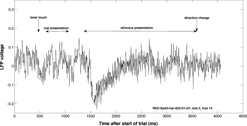
Figure 1 shows a single raw data before cutting. Each trial includes 682 features in time domain from the stimulus onset time for the analysis.

Fig. 1.

A sample of raw local field potential recorded during the experiment. Point of stimulus onset is in 1085 ms and the number of features is selected as 682 ms in time domain from the time of stimulus presentation onset

In addition to anatomical position, physiological characteristics must also be considered for specifying the correct area for recording. The high percentage of neurons in MT area is characterized by a direction selectivity of a moving visual stimulus (Martinez-Trujillo and Treue 2004; Albright 1984). Therefore, one of the specified properties to ensure that the electrodes are placed in MT area is directional selectivity of neurons in this area.

According to this observation, most of the neurons in MT area can be fitted well with a bell-shaped tuning curve; therefore, fitting the neuronal response tuning curves with Gaussian functions is a strong statistical quantitative analysis. The Gaussian function provides an estimation of the tuning curves in MT area (Albright 1984). In this study, directional tuning curve for eight movement directions of random dot patterns (RDPs) at 45 degree intervals were fitted with Gaussian curve with the mean of θ₀ (the preferred direction), and standard deviation Δθ (the curve width) by the given information about selectivity of neurons in any recording trial. The monkey was trained to attend to a moving RDP which was moved in one of the possible eight directions (0°, 45°, 90°, 135°, 180°, 225°, 270°, 315°). Then, the data were recorded in two attentional conditions while each condition contained 8 directions. In the present study, the tuning curve of firing rates along eight directions was used and the channels that fitted well with Gaussian function were selected in order to be sure that the electrode has been placed in MT area.

The goodness of fitting the curves was assessed using r-square (coefficient of determination for evaluating goodness of fitting). It has been found that all of the channels do not always coincide with the Gaussian function. Here in, the channels were selected such that their r-square remained above 0.75.

In total 6610 trials were divided into two equal groups, the training set and the test set. The random sub-sampling method has been used for validation of the methods. The 6610 trials permuted across both of training and test sets in any run. It is worth mentioning that the problems of overfitting are noticed, however, the idea of using different methods for classification and obtaining similar results verifies the reliability of the obtained results. In addition we have checked for the cases of overfittings (like the number of SVs in SVM etc). Since the overfitting could provide unreliable results among different runs, a validation strategy over each 15 runs has been utilized to prevent any inaccurate outcome. Furthermore, to have enough number of observations per parameter, we limited the maximum number of selected features to 200.

Task

All trials started with presentation of a fixation-point in the middle of the screen for the duration of 130 ms. A cue was appeared for the duration of 455 ms indicating the position of the stimulus that the monkey had to attend. After that, two moving RDPs were presented in the screen, one inside the receptive field (RF) and one outside the RF of the population neurons placing near the electrode tips (both RDPs moved in the same direction among 8 possible directions). Using the cue at the beginning of each trial, the monkey was pushed to focus his attention to the cued RDP. The monkey had to report the change (the direction change) of the cued pattern by pushing a lever and ignore the change in the other pattern. The direction change could happen in a random time between 650 and 3250 ms after the two RDPs appeared. Indeed, the monkey was trained to discern attention to inside RF or outside RF according to the position of the cue.

The task has been shown graphically in Fig. 2.

Fig. 2.

Task of the data recording. All of the experimental runs were begun with fixation-point. For two classes (attention inside RF and attention outside RF), RDPs were displayed inside RF and outside RF, respectively. After the presentation of the cue, RDPs were displayed in two places. The monkey had to report the direction change of the cued pattern and ignore the change in the other one

Results

Here, we have evaluated the possibility of decoding of the attended position of the stimuli from the LFP signals recorded from area MT of a macaque monkey using machine learning approaches. We extracted and identified specific features in different time−frequency domains which one is carrying information on spatial attention of the monkey. This prediction has an important role in understanding of the physiological mechanisms underlying cognitive brain functions.

For the analysis, we cut the part of the raw LFP signals which was related to exact time of the monkey’s attention in spatial attention task. These signals contain 682 sample points (features) in time (the sampling rate of recording was at 1 kHz, so the duration of the LFP signals was 682 ms). There were 6610 trials available for the processing in two attentional conditions: attention inside RF and attention outside RF. We divided these trials to equal two groups, training set and test set. 3305 trials in the training set and 3305 trials in the test set were analyzed. To evaluate the decoding accuracies, the sequence of training and test trials was randomly permuted 15 times before classification. The results of classification are the average of 15 different runs with different training/test sets. In different time−frequency domains, the feature vectors and the related labels in the training set were used to train the different classifiers and the performance of decoding was evaluated in the test set.

Feature extraction was done in spectrogram, CWT, and energy wavelet domains. Also, analysis was implemented for time domain. Feature selection was applied using four criteria (T-test, Entropy, ROC, and Bhattacharyya) for different classifiers such as SVM, KNN, naïve Bayes, LDA, QDA with their different options. Finally, after feature extraction, the number of the features were 682, 1161, 21,824, 21,824, from time, spectrogram, CWT, and energy wavelet, respectively. The best results were obtained using the T-test in time and spectrogram (as can be seen from the results reported in the next sections). Different classifiers were applied to find the best efficiency and accuracy in the time and frequency domains. As can be seen the results of some feature selection methods are better for some classifiers than for others. Feature selection methods are independent of the classifiers, so different accuracies obtained from different classifiers are due to the power of the classifiers themselves.

Decoding in time

Table 1 represents the results for the best classifier in time domain. The following classifiers have been evaluated in this experiment repeatedly: SVM classifier with its kernels (linear, RBF, and polynomial with different sigma and order factors), KNN with different distances and rules, naïve Bayes with different distributions and priors, LDA, and QDA.

Table 1.

Results of the evaluation of the best classifier in time domain

Classifier	Selected criterion	Performance	TP rate	TN rate	FP rate	FN rate	Precision
KNN (k = 1, distance = Euclidean, rule = nearest)	T-test	0.845	0.8265	0.8658	0.1342	0.1735	0.8732

The best classifier was KNN (K = 1, the rule: nearest, and the distance: Euclidean) in the time domain.

The results indicate that a high classification accuracy was achieved in this case (>84.5 % correct for classifying the LFP signals in time domain).

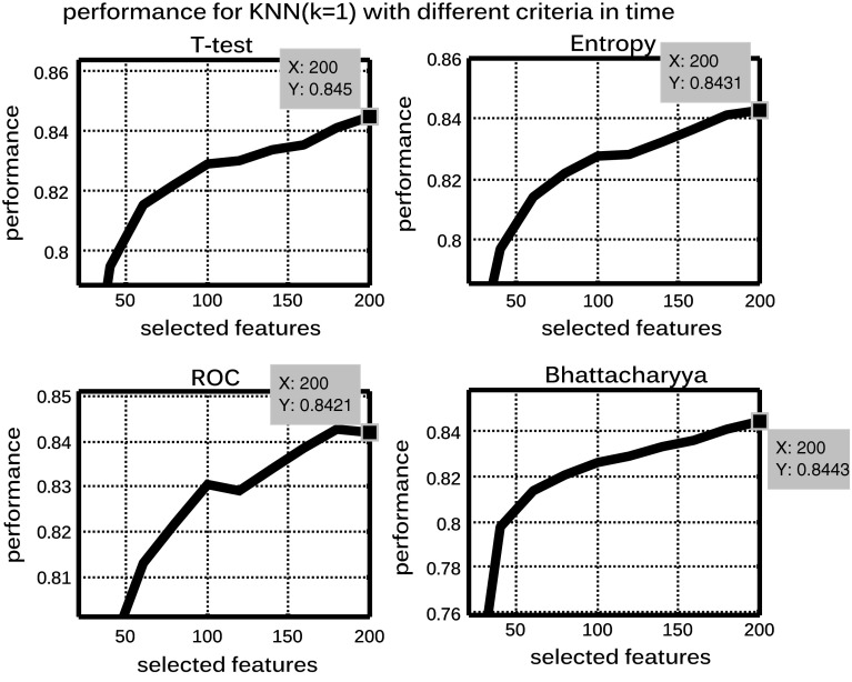
The features were selected by four criteria (T-test, Entropy, ROC, and Bhattacharyya). The best criterion was T-test with 200 features and above 84.5 % performance for KNN (K = 1, the rule: nearest, and the distance: Euclidean), as shown in Fig. 3.

Fig. 3.

The trend of performances versus the number of selected features using four criteria (T-test, Entropy, ROC, and Bhattacharyya) for KNN (K = 1, the distance: Euclidean, and the rule: nearest) for the time-domain features. The best criterion is T-test with 200 features and above 84.5 % performance

The experimental results of classification present the feasibility of selecting a feature set for discriminating the location of attention (inside and outside RF). Generally, if we select the more features, the better accuracy is achieved. But it is observed that this increasing is saturated in the certain point and we neglected from one or two percent of accuracy for having the less number of selected features (lower complexity). We preferred to select the less number of features rather than a little better performance. The goal of showing performance as a function of the number of features is finding the highest performance for the minimum number of selected features. The trend of performance versus the number of selected features has been shown in Fig. 3 for the time domain features.

Decoding in time−frequency domain by using spectrogram features

Different experiments were performed and the best classifier was selected with the highest accuracy in time−frequency domain. The SVM classifier with its kernels (linear, RBF and polynomial) was used and its sigma and other factors were changed in both RBF and polynomial kernels. KNN classifier with different number of the nearest neighbors (K), different measurement distances, and the rules was also provided. Bayesian classifier with different distributions and priors, and LDA and QDA were also tested. Finally, SVM (kernel: polynomial, order = 3, and method: LS) was selected as the best classifier in spectrogram, as indicated in Table 2.

Table 2.

Results of the evaluation of the best classifier for the spectrogram

Classifier	Selected criterion	Performance	TP rate	TN rate	FP rate	FN rate	Precision
SVM (Kernel function = polynomial, Method = LS, order = 3)	T-test	0.8297	0.8191	0.8413	0.1587	0.1809	0.8461

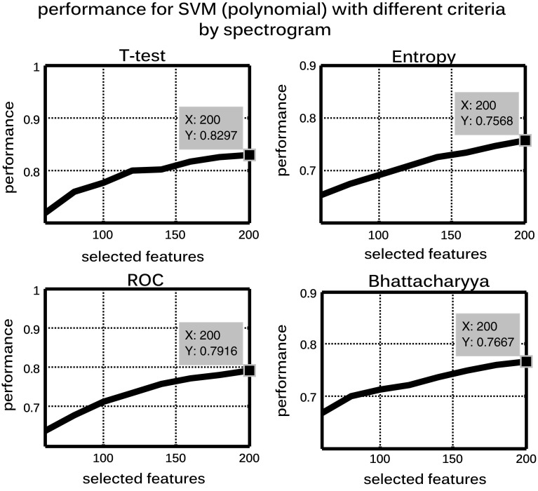
Feature selection was done by four criteria (T-test, Entropy, ROC, and Bhattacharyya) for the selected classifier. The best criterion was T-test with 200 features and 82.9 % performance for the selection of the least number of features (Fig. 4).

Fig. 4.

The trend of performances versus the number of selected features using four criteria (T-test, Entropy, ROC, and Bhattacharyya) for SVM (kernel: polynomial, order = 3) for the spectrogram. The best criterion is T-test with 200 features and 82.9 % performance

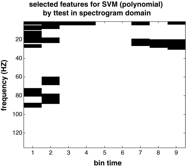
Also, the map of selected features has been shown for the best criterion (T-test), in Fig. 5. The number of the selected features is 200 with feature selection method. Results show that the maximum information is in low frequency features during the whole time period. Also, the figure shows that many frequency features are informative in the initial time interval.

Fig. 5.

The selected features with SVM (kernel: polynomial and order = 3) in time−frequency domain (spectrogram). 200 features were selected by T-test. Each time bin is about 128 ms for this plot. Low frequency features in the whole time period and most of the frequency features at the initial time interval are informative

The size of each time bin was 128 ms in this analysis. The number of overlap was about half of selected window length, 64 ms. The overlap is used to measure each part of the signal twice, when it is in the middle of the window and at the ends of the window. There were 9 time windows. The sampling frequency was normalized.

The present results showed that the selective visual attention revealed an increase of oscillations in the frequency band below approximately 95 Hz at initial time period and below about 35 Hz for the whole time period in population of visual cortical neurons. This indicated that oscillations of specified area help to optimize processing under attention.

Decoding in time−frequency domain by using CWT features

We examined how the attention to one of the two separate positions of stimuli in the visual field, attention inside RF and attention outside RF, could be decoded from the LFP signals. To find out whether two classes of spatial selective attention can be significantly distinguished in individual trials, we classified the recorded data by different classifiers. For this indication, information about the performance of classifiers is useful. Furthermore, we demonstrated relation between performance and the number of features used for classification. The features were extracted using CWT method and were evaluated in this subsection.

Similar to previous subsection, the different classifiers with their options were tested which are the SVM classifier with its kernels (linear, RBF, and polynomial), different sigma, and order factors; KNN classifier with different number of the nearest neighbors (K), different distances, and the rules; Bayesian classifier with the different distributions and the priors; LDA, and QDA for the CWT features. The best selected classifier was SVM (kernel: RBF and sigma = 36) in time−frequency domain with CWT features based on the performance of the classifier. The results have been summarized in Table 3.

Table 3.

Results of the evaluation of the best classifier in CWT

Classifier	Selected criterion	Performance	TP rate	TN rate	FP rate	FN rate	Precision
SVM (Kernel function = RBF, method = LS, Sigma = 36	Bhattacharyya	0.7074	0.7057	0.7093	0.2907	0.2943	0.7124

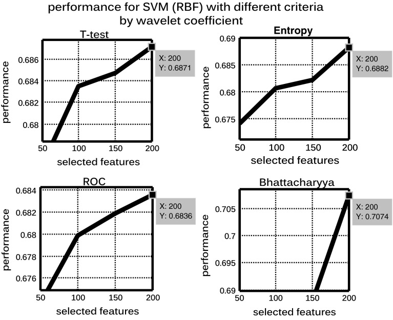
Different criteria were tested to select the least number of the features in this case too (Fig. 6). Best criterion was Bhattacharyya with 200 features and 70.7 % performance in CWT. Feature selection curves were increased by the number of features, so that they were saturated in a certain number of features.

Fig. 6.

The trend of performances versus the number of selected features using four criteria (T-test, Entropy, ROC, and Bhattacharyya) for SVM (kernel: RBF, sigma = 36) for the wavelet coefficient features. The best criterion is Bhattacharyya with 200 features and 70.7 % performance

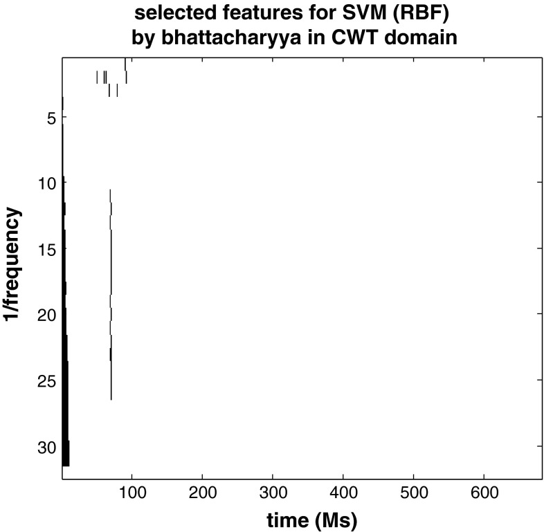
Figure 7 shows the selected features by Bhattacharyya for SVM (kernel: RBF, sigma = 36) in time−frequency domain (CWT). The results indicate that the maximum information is mainly in low frequency features at initial time interval.

Fig. 7.

The selected features in time−frequency domain (CWT) with SVM (kernel: RBF, sigma = 36). 200 features selected with Bhattacharyya criterion. Low frequency features have useful information regarding the visual attention at initial time interval

Decoding in time−frequency domain by using energy wavelet features

In this section, scalogram features were classified by the following classifiers: SVM, KNN, naïve Bayes, LDA and QDA. The mentioned classifiers and their different options were tested. Finally, KNN (k = 1, the distance: correlation, and the rule: nearest) was obtained the highest accuracy as shown in Table 4.

Table 4.

Results of the evaluation of the best classifiers in energy wavelet

Classifier	Selected criterion	Performance	TP rate	TN rate	FP rate	FN rate	Precision
KNN (k = 1, distance = correlation, rule = nearest)	T-test	0.6636	0.6671	0.6603	0.3397	0.3329	0.6588

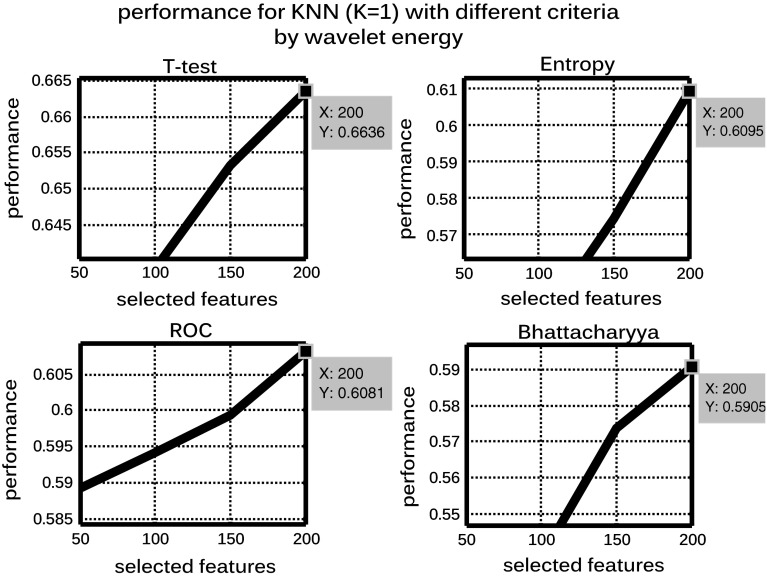
Four criteria (T-test, Entropy, ROC, and Bhattacharyya) were assessed to choose the highest accuracy of classification in time−frequency domain (scalogram) for KNN (K = 1, the distance: correlation, and the rule: nearest). The best criterion was T-test with 200 features and 66.3 % performance, as shown in Fig. 8.

Fig. 8.

The trend of performances versus the number of selected features using four criteria (T-test, Entropy, ROC, and Bhattacharyya) for KNN (K = 1, the distribution: correlation, and the rule: nearest) for the wavelet energy features. The best criterion is T-test with 200 features and 66.3 % performance

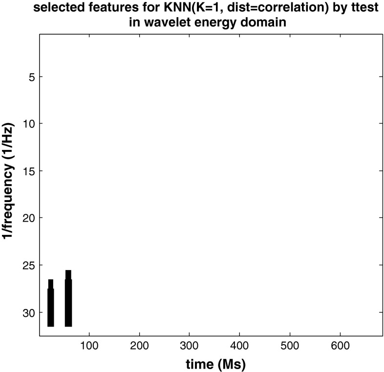
The selected features were presented in time−frequency domain (energy wavelet) in Fig. 9. 200 features were selected by T-test criterion. The results revealed that the low frequency features at the initial time interval have higher information for the decoding of attention in this case.

Fig. 9.

The selected features in time−frequency domain (energy wavelet) with KNN (K = 1, the distribution: correlation, and the rule: nearest). 200 features were selected by T-test criterion. The low frequency features at the initial time interval have higher information about the decoding of spatial attention

Feature selection by using windowing method in time

We explored the decoding of switching attention of a monkey from the inside to the outside RF. The results indicated a modulation in the early time intervals. This result was observed by the available high performance of selected features for the classification by using windowing method in time domain.

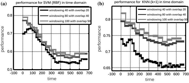
In this part, different lengths and overlaps were tested to select a proper window size in order to create high accuracy of classification in time domain. Indeed, the data size was reduced and speed of processing was increased by this method. In this section, windowing represents continuous feature selection for SVM (kernel: RBF, Sigma = 7, and method: LS). Results showed performance is high at initial time period of the task (Fig. 10a).

Fig. 10.

a feature selection by windowing for SVM (kernel: RBF, Sigma = 7, and method: LS). Results are shown for the three window size choices. Performance is high at initial time period. b Feature selection by windowing for KNN (K = 1, the distribution: Euclidean, and the rule: nearest). Results are shown for the three window size choices. Initial time interval has high performance

Also, feature selection by windowing is shown for KNN (K = 1, the distribution: Euclidean, and the rule: nearest). Similarly, initial time interval has high performance (Fig. 10b).

In windowing method, the choice of different parameters to slide signal including the number of windows, the length of the windows, and the size of overlap between selected-windows has extraordinary importance on the performance of the data processing. We used three windows for data sliding. The number of features in any window was 40, 80, and 100, respectively. In the three windowing analysis, overlaps of 20, 40, and 50 were considered respectively. For example, in the first windowing, the size of selected window included 40 features in time and each window with its adjacent window had 20 time points overlap. According to the 682 features in time and overlaps, the number of windows was 13, 17, and 34, respectively for three experiments.

Discussion and conclusions

The local field potentials are interesting source of brain activities which have been used in many decoding applications. In this study, we have studied and evaluated the LFP signals from the visual system to decode of attention. In this work, available data including LFPs recorded from MT of a monkey’s brain were analyzed. Informative regions and features have been shown by feature extraction and feature selection in both time and frequency domains. In other words, decoding has been executed by these techniques. Feature extraction was performed using STFT, CWT, and wavelet energy. Feature selection was applied using four different criteria (T-test, Entropy, ROC, and Bhattacharyya). The least number of features were selected for classification. The results show that the best performance would be obtained in time and spectrogram domain.

It is possible to decode the devotion of attention to one of two places in visual field by LFP signals over MT area of monkey. Single trials are classified in two classes, attention inside RF and outside RF. Finally, features supported the high accuracy of classification including 84.5 % performance for KNN in time, 82.9 % performance for SVM in spectrogram, 70.7 % performance for SVM in CWT, and 60.3 % performance for KNN in wavelet energy.

The number of the features were 682, 1161, 21,824, 21,824, in time, spectrogram, CWT, and energy wavelet domains, respectively. The number of the features refers to the total number of available features after feature extraction methods. Then we selected the minimum features (200 features) for having the best performance using different feature selection approaches. The optimal number of features was selected based on four criteria (T-test, Entropy, ROC, and Bhattacharyya). Finally, 200 of 682 features in time, 200 of 1161 features in spectrogram, 200 of 21,824 features in CWT, and 200 of 21,824 features in wavelet energy was selected during these methods.

In summary, T-test with 84.5 % performance in time, T-test with 82.9 % performance in spectrogram, Bhattacharyya with 70.7 % performance in CWT, and T-test with 66.3 % performance in wavelet energy were as the best criteria and the least number of features. In different domains, the best choices of classifiers were: KNN (K = 1, distance: Euclidean) in time, SVM (kernel: polynomial, order = 3) in spectrogram, SVM (kernel: RBF, sigma = 36) in CWT, KNN (K = 1, distance: correlation) in wavelet energy.

Also, feature selection was investigated by data windowing in time domain. It is concluded that the data are informative for the decoding of spatial attention. Maximum information is located at initial time intervals. Feature selection was used by windowing and SVM (kernel: RBF, Sigma = 7, and method: LS) and KNN (K = 1, distance: Euclidean). High performance has been obtained in the mentioned interval.

Using just one method of classification could provide similar results in terms of the selected features in different domains. We wanted to be sure that the selected features are not based on the tuning of a special method. Therefore the results are reliable. We used signals in different time−frequency domains and selected the best classifier with the higher performance. Then we selected the least number of features (200 features) with selected classifier and four criteria in any domain. Finally, we mapped the least features (200 features). Totally, the same results of maps obtained in spectrogram, CWT, and energy wavelet. The best performances have been summarized in the following Table 5.

Table 5.

Evaluation results of the best classifiers using the least number of selected features (200) for different methods

Domain	Classifier	The number of selected features	Criterion	Performance %
Time	KNN (k = 1, distance = Euclidean, rule = nearest)	200	T-test	84.5
Spectrogram	SVM (Kernel function = polynomial, Method = LS, order = 3)	200	T-test	82.9
CWT	SVM (Kernel function = RBF, method = LS, Sigma = 36)	200	Bhattacharyya	70.7
Energy wavelet	KNN (k = 1,distance = correlation, rule = nearest)	200	T-test	66.3

The best results are related to spectrogram (82.9 %) and time domain (84.5 %) for having the highest performance.

We have studied the best performance and the least number of features for any criterion; as it is expected, the selected criteria based on the best performance would be different. Finally, the selected criteria are T-test in time, spectrogram, and energy wavelet and Bhattacharyya in CWT. Overall, different time−frequency domains have similar results in the specified area of feature selection, at low frequency components at initial time intervals of the trials.

Furthermore, the informative frequency ranges are below 35 Hz at the whole time period and below 95 Hz at initial time period in spectrogram, below 100 Hz in CWT, and below 40 Hz in scalogram. The other frequency bands carry relatively less information about spatial attention.

Our approach was to build a neural decoding from visual attention, and to evaluate whether this method could predict the attentional focus of the monkey at a level of accuracy higher than expected by chance. The informative areas in Figs. 5, 7 and 9 provide the most conclusive part of the results. Indeed, we found the least number of features by selection features to discriminate attentional focus of the monkey for the test trials. The specified features have the strongest contribution to the decoding performance and to predict the locus of attention. This would indicate that there is some helpful information about two positions (attention inside and attention outside of RF) in the selected features. The influence of work on the selected features in different time−frequencies domains would suggest LFPs to decode attentional state.

In summary, results showed that the maximum information was located at low frequency features at initial time interval in different domains. It was shown that LFP signals can be informative about visual attention in the MT of the monkey. This signal can be used to decode of spatial attention. The current study provides general discussion of the classification of LFP signals. It determined features which contain useful information about spatial attention. In the other word, these signals were evaluated from the classification point of view to connect brain reaction and accuracy. This study also gave insight into the importance mechanisms of neuronal computation.

Our approach of decoding the locus of attention using windowing in spectrogram, CWT, and scalogram indicates the dynamics of attentional modulation in LFP signals across the time course of the trials.

Figures 5, 7 and 9 show the dynamics of the selected features in time. The information has been concentrated in specified area of different domains in different time bins (mainly the low frequency features at the initial time interval have higher information about the decoding of spatial attention).

According to the previous suggestions in other papers, valuable methods can be performed on signals of brain for future works. For example, the windowing method in the frequency domains of feature selection can be proposed. As another suggestion, Autoregressive (AR) and discrete wavelet transform (DWT) techniques can be used for feature extraction. Also, combination of neural networks and different classifiers can be helpful for classification to improve the results.

References

- Albright TD. Direction and orientation selectivity of neurons in visual area MT of the macaque. J Neurophysiol. 1984;52(6):1106–1130. doi: 10.1152/jn.1984.52.6.1106. [DOI] [PubMed] [Google Scholar]
- Belitski A, Gretton A, Magri C, Murayama Y, Montemurro M, Logothetis N, Panzeri S. Low-frequency local field potentials and spikes in primary visual cortex convey independent visual information. J Neurosci. 2008;28(22):5696–5709. doi: 10.1523/JNEUROSCI.0009-08.2008. [DOI] [PMC free article] [PubMed] [Google Scholar]
- Belitski A, Panzeri S, Magri C, Logothetis NK, Kayser C. Sensory information in local field potentials and spikes from visual and auditory cortices: time scales and frequency bands. J Comput Neurosci. 2010;29(3):533–545. doi: 10.1007/s10827-010-0230-y. [DOI] [PMC free article] [PubMed] [Google Scholar]
- Bisley JW. The neural basis of visual attention. J Physiol. 2011;589(1):49–57. doi: 10.1113/jphysiol.2010.192666. [DOI] [PMC free article] [PubMed] [Google Scholar]
- Carrasco M. Visual attention: the past 25 years. Vis Res. 2011;51:1484–1525. doi: 10.1016/j.visres.2011.04.012. [DOI] [PMC free article] [PubMed] [Google Scholar]
- Chen Z, et al. An empirical EEG analysis in brain death diagnosis for adults. Cogn Neurodyn. 2008;2(3):257–271. doi: 10.1007/s11571-008-9047-z. [DOI] [PMC free article] [PubMed] [Google Scholar]
- Choi E, Lee C. Feature extraction based on the Bhattacharyya distance. Pattern Recogn. 2003;36(8):1703–1709. doi: 10.1016/S0031-3203(03)00035-9. [DOI] [Google Scholar]
- Cotic M, Chiu AWL, Jahromi SS, Carlen PL, Bardakjian BL. Common time−frequency analysis of local field potential and pyramidal cell activity in seizure-like events of the rat hippocampus. J Neural Eng. 2011;8(4):046024. doi: 10.1088/1741-2560/8/4/046024. [DOI] [PubMed] [Google Scholar]
- Coyle D, Prasad G, McGinnity TM. A time-frequency approach to feature extraction for a brain–computer interface with a comparative analysis of performance measures. EURASIP J Appl Signal Process. 2005;19:3141–3151. doi: 10.1155/ASP.2005.3141. [DOI] [Google Scholar]
- Dastidar SGh, Adeli H, Dadmehr N. Mixed-band wavelet-chaos-neural network methodology for epilepsy and epileptic seizure detection. IEEE Trans Biomed Eng. 2007;54:1545–1551. doi: 10.1109/TBME.2007.891945. [DOI] [PubMed] [Google Scholar]
- Duda RO, Hart PE, Stork DG. Pattern classification. 2. London: Wiley; 2000. [Google Scholar]
- Engel AK, Moll CKE, Fried I, Ojemann GA. Invasive recordings from the human brain: clinical insights and beyond. Nat Rev Neurosci. 2005;6:35–47. doi: 10.1038/nrn1585. [DOI] [PubMed] [Google Scholar]
- Esghaei M, Daliri MR. Decoding of visual attention from LFP signals of macaque MT. PLoS One. 2014;9(6):e100381. doi: 10.1371/journal.pone.0100381. [DOI] [PMC free article] [PubMed] [Google Scholar]
- Flint RD, Lindberg EW, Jordan LR, Miller LE, Slutzky MW (2012) Accurate decoding of reaching movements from field potentials in the absence of spikes. J Neural Eng 9(4):046006 [DOI] [PMC free article] [PubMed]
- Gu Y, Liljenström H. A neural network model of attention-modulated neurodynamics. Cogn Neurodyn. 2007;1(4):275–285. doi: 10.1007/s11571-007-9028-7. [DOI] [PMC free article] [PubMed] [Google Scholar]
- Herrington TM, Assad JA. Neural activity in the middle temporal area and lateral intraparietal area during endogenously cued shifts of attention. J Neurosci. 2009;29(45):14160–14176. doi: 10.1523/JNEUROSCI.1916-09.2009. [DOI] [PMC free article] [PubMed] [Google Scholar]
- Ince NF, Gupta R, Arica S, Tewfik AH, Ashe J, Pellizzer G. High accuracy decoding of movement target direction in non-human primates based on common spatial patterns of local field potentials. PLoS One. 2010;5(12):e14384. doi: 10.1371/journal.pone.0014384. [DOI] [PMC free article] [PubMed] [Google Scholar]
- Kajikawa Y, Schroeder ChE. How local is the local field potential? Neuron. 2011;72(5):847–858. doi: 10.1016/j.neuron.2011.09.029. [DOI] [PMC free article] [PubMed] [Google Scholar]
- Kaliukhovich DA, Vogels R (2013) Decoding of repeated objects from local field potentials in macaque inferior temporal cortex. Plos One 8(9):e74665 [DOI] [PMC free article] [PubMed]
- Katzner S, Nauhaus I, Benucci A, Bonin V, Ringach DL, Carandini M. Local origin of field potentials in visual cortex. Neuron. 2009;61:35–41. doi: 10.1016/j.neuron.2008.11.016. [DOI] [PMC free article] [PubMed] [Google Scholar]
- Kellis S, Miller K, Thomson K, Brown R, House P, Greger B. Decoding spoken words using local field potentials recorded from the cortical surface. J Neural Eng. 2010;7(5):056007. doi: 10.1088/1741-2560/7/5/056007. [DOI] [PMC free article] [PubMed] [Google Scholar]
- Khayat PS, Niebergall R, Trujillo JCM. Frequency-dependent attentional modulation of local field potential signals in macaque area MT. J Neurosci. 2010;30(20):7037–7048. doi: 10.1523/JNEUROSCI.0404-10.2010. [DOI] [PMC free article] [PubMed] [Google Scholar]
- Kotsiantis SB. Supervised machine learning: a review of classification techniques. Inform Slov. 2007;31(3):249–268. [Google Scholar]
- Liu J, Newsome WT. Local field potential in cortical area MT: stimulus tuning and behavioral correlations. J Neurosci. 2006;26(30):7779–7790. doi: 10.1523/JNEUROSCI.5052-05.2006. [DOI] [PMC free article] [PubMed] [Google Scholar]
- Manyakov NV, Vogels R, Van Hulle MM. Decoding stimulus–reward pairing from local field potentials recorded from monkey visual cortex. IEEE Trans Neural Netw. 2010;21(12):1892–1902. doi: 10.1109/TNN.2010.2078834. [DOI] [PubMed] [Google Scholar]
- Martinez-Trujillo JC, Treue S. Feature-based attention increases the selectivity of population responses in primate visual cortex. Curr Biol. 2004;14:744–751. doi: 10.1016/j.cub.2004.04.028. [DOI] [PubMed] [Google Scholar]
- Mehring C, Rickert J, Vaadia E, Oliveira SC, Aertsen A, Rotter S. Inference of hand movements from local field potentials in monkey motor cortex. Nat Neurosci. 2003;6(12):1253–1254. doi: 10.1038/nn1158. [DOI] [PubMed] [Google Scholar]
- Mitzdorf U. Properties of the evoked potential generators: current source-density analysis of visually evoked potentials in the cat cortex. Int J Neurosci. 1987;33:33–59. doi: 10.3109/00207458708985928. [DOI] [PubMed] [Google Scholar]
- Mollazadeh M, Aggarwal V, Singhal G, Law A, Davidson A, Schieber M, Thakor N (2008) Spectral modulation of LFP activity in M1 during dexterous finger movements. In: 30th Annual international IEEE EMBS conference Vancouver, Canada, pp 50314–50317 [DOI] [PubMed]
- Nakatani H, Orlandi N, Leeuwen CV. Precisely timed oculomotor and parietal EEG activity in perceptual switching. Cogn Neurodyn. 2011;5:399–409. doi: 10.1007/s11571-011-9168-7. [DOI] [PMC free article] [PubMed] [Google Scholar]
- Rasch M, Logthetis NK, Kreiman G. From neurons to circuits: linear estimation of local field potentials. J Neurosci. 2009;29(44):13785–13796. doi: 10.1523/JNEUROSCI.2390-09.2009. [DOI] [PMC free article] [PubMed] [Google Scholar]
- Seidemann E, Newsome WT. Effect of spatial attention on the responses of area MT neurons. J Neurophysiol. 1999;81:1783–1794. doi: 10.1152/jn.1999.81.4.1783. [DOI] [PubMed] [Google Scholar]
- Shipp S (2004) The brain circuitry of attention. Trends Cogn Sci 8(5):223–230 [DOI] [PubMed]
- Song Y, Huang J, Zhou D, Zha H, Giles CL (2007) IKNN: informative K-nearest neighbor pattern classification. In: 11th European conference on principles and practice of knowledge discovery in databases, Berlin, pp 248–264
- Starzacher A, Rinner B (2008) Evaluating KNN, LDA and QDA classification for embedded online feature fusion. In: International conference on intelligent sensors, sensor networks and information processing, Australia, pp 85–90
- Sundberg KA, Mitchell JF, Reynolds JH. Spatial attention modulates center–surround interactions in macaque visual area V4. Neuron. 2009;61(6):952–963. doi: 10.1016/j.neuron.2009.02.023. [DOI] [PMC free article] [PubMed] [Google Scholar]
- Taghizadeh-Sarabi M, Daliri MR, Niksirat KS (2015) Decoding objects of basic categories from electroencephalographic signals using wavelet transform and support vector machines. Brain Topogr 28(1):33–46 [DOI] [PubMed]
- Theodoridis S, Koutroumbas K. Pattern classification. 3. London: Academic Press; 2006. [Google Scholar]
- Treue S, Maunsell JHR. Effects of attention on the processing of motion in macaque middle temporal and medial superior temporal visual cortical areas. J Neurosci. 1999;19(17):7591–7602. doi: 10.1523/JNEUROSCI.19-17-07591.1999. [DOI] [PMC free article] [PubMed] [Google Scholar]
- Vecera SP, Rizzo M. Spatial attention: normal processes and their breakdown. Neurol Clin. 2003;21(3):575–607. doi: 10.1016/S0733-8619(02)00103-2. [DOI] [PubMed] [Google Scholar]
- Wang Z, Logothetis NK, Liang H. Decoding a bistable percept with integrated time-frequency representation of single-trial local field potential. J Neural Eng. 2008;5:433–442. doi: 10.1088/1741-2560/5/4/008. [DOI] [PubMed] [Google Scholar]
- Wang Z, Logothetis NK, Liang H. Extraction of percept-related induced local field potential during spontaneously reversing perception. Neural Netw. 2009;22:720–727. doi: 10.1016/j.neunet.2009.06.037. [DOI] [PubMed] [Google Scholar]
- Xu B, Song A. Pattern recognition of motor imagery EEG using wavelet transform. J Biomed Sci Eng. 2008;1:64–67. doi: 10.4236/jbise.2008.11010. [DOI] [Google Scholar]
- Zhen Z, Zeng X, Wang H, Han L (2011) A global evaluation criterion for feature selection in text categorization using Kullback–Leibler divergence. In: International conference of soft computing and pattern recognition, China, pp 440–445