

Significance
The activity of a brain—or even a small region of a brain devoted to a particular task—cannot be just the summed activity of many independent neurons. Here we use methods from statistical physics to describe the collective activity in the retina as it responds to complex inputs such as those encountered in the natural environment. We find that the distribution of messages that the retina sends to the brain is very special, mathematically equivalent to the behavior of a material near a critical point in its phase diagram.
Keywords: entropy, information, neural networks, Monte Carlo, correlation
Abstract
The activity of a neural network is defined by patterns of spiking and silence from the individual neurons. Because spikes are (relatively) sparse, patterns of activity with increasing numbers of spikes are less probable, but, with more spikes, the number of possible patterns increases. This tradeoff between probability and numerosity is mathematically equivalent to the relationship between entropy and energy in statistical physics. We construct this relationship for populations of up to N = 160 neurons in a small patch of the vertebrate retina, using a combination of direct and model-based analyses of experiments on the response of this network to naturalistic movies. We see signs of a thermodynamic limit, where the entropy per neuron approaches a smooth function of the energy per neuron as N increases. The form of this function corresponds to the distribution of activity being poised near an unusual kind of critical point. We suggest further tests of criticality, and give a brief discussion of its functional significance.
Our perception of the world seems a coherent whole, yet it is built out of the activities of thousands or even millions of neurons, and the same is true for our memories, thoughts, and actions. It is difficult to understand the emergence of behavioral and phenomenal coherence unless the underlying neural activity also is coherent. Put simply, the activity of a brain—or even a small region of a brain devoted to a particular task—cannot be just the summed activity of many independent neurons. How do we describe this collective activity?
Statistical mechanics provides a language for connecting the interactions among microscopic degrees of freedom to the macroscopic behavior of matter. It provides a quantitative theory of how a rigid solid emerges from the interactions between atoms, how a magnet emerges from the interactions between electron spins, and so on (1, 2). These are all collective phenomena: There is no sense in which a small cluster of molecules is solid or liquid; rather, solid and liquid are statements about the joint behaviors of many, many molecules.
At the core of equilibrium statistical mechanics is the Boltzmann distribution, which describes the probability of finding a system in any one of its possible microscopic states. As we consider systems with larger and larger numbers of degrees of freedom, this probabilistic description converges onto a deterministic, thermodynamic description. In the emergence of thermodynamics from statistical mechanics, many microscopic details are lost, and many systems that differ in their microscopic constituents nonetheless exhibit quantitatively similar thermodynamic behavior. Perhaps the oldest example of this idea is the “law of corresponding states” (3).
The power of statistical mechanics to describe collective, emergent phenomena in the inanimate world led many people to hope that it might also provide a natural language for describing networks of neurons (4–6). However, if one takes the language of statistical mechanics seriously, then as we consider networks with larger and larger numbers of neurons, we should see the emergence of something like thermodynamics.
Theory
At first sight, the notion of a thermodynamics for neural networks seems hopeless. Thermodynamics is about temperature and heat, both of which are irrelevant to the dynamics of these complex, nonequilibrium systems. However, all of the thermodynamic variables that we can measure in an equilibrium system can be calculated from the Boltzmann distribution, and hence statements about thermodynamics are equivalent to statements about this underlying probability distribution. It is then only a small jump to realize that all probability distributions over N variables can have an associated thermodynamics in the limit. This link between probability and thermodynamics is well-studied by mathematical physicists (7), and has been a useful guide to the analysis of experiments on dynamical systems (8, 9).
To be concrete, consider a system with N elements; each element is described by a state , and the state of the entire system is . We are interested in the probability that we will find the system in any one of its possible states. It is natural to think not about the probability itself but about its logarithm,
| [1] |
In an equilibrium system, this is precisely the energy of each state (in units of ), but we can define this energy for any probability distribution. As discussed in detail in Supporting Information, all of thermodynamics can be derived from the distribution of these energies. Specifically, what matters is how many states have close to a particular value E. We can count this number of states, , or more simply the number of states with energy less than E, . Then we can define a microcanonical entropy . If we imagine a family of systems in which the number of degrees of freedom N varies, then a thermodynamic limit will exist provided that both the entropy and the energy are proportional to N at large N. The existence of this limit is by no means guaranteed.
In most systems, including the networks that we study here, there are few states with high probability, and many more states with low probability. At large N, the competition between decreasing probability and increasing numerosity picks out a special value of , which is the energy of the typical states that we actually see; is the solution to
| [2] |
For most systems, the energy has only small fluctuations around , , and, in this sense, most of the states that we see have the same value of log probability per degree of freedom. However, hidden in the function are all of the parameters describing the interactions among the N degrees of freedom in the system. At special values of these parameters, , and the variance of E diverges as N becomes large. This is a critical point, and it is mathematically equivalent to the divergence of the specific heat in an equilibrium system (10).
These observations focus our attention on the “density of states” . Rather than asking how often we see specific combinations of spiking and silence in the network, we ask how many states there are with a particular probability.
Experimental Example
The vertebrate retina offers a unique system in which the activity of most of the neurons comprising a local circuit can be monitored simultaneously using multielectrode array recordings. As described more fully in ref. 11, we stimulated salamander retina with naturalistic grayscale movies of fish swimming in a tank (Fig. 1A), while recording from 100 to 200 retinal ganglion cells (RGCs); additional experiments used artificial stimulus ensembles, as described in Supporting Information. Sorting the raw data (12), we identified spikes from 160 neurons whose activity passed our quality checks and was stable for the whole 2 h duration of the experiment; a segment of the data is shown in Fig. 1B. These experiments monitored a substantial fraction of the RGCs in the area of the retina from which we record, capturing the behavior of an almost complete local population responsible for encoding a small patch of the visual world. The experiment collected a total of spikes, and time was discretized in bins of duration ; all of the results discussed below are substantially the same at and (Fig. S1). For each neuron , in a bin denotes that the neuron emitted at least one spike, and denotes that it was silent.
Fig. 1.

Counting states in the response of RGCs. (A) A single frame from the naturalistic movie; red ellipse indicates the approximate extent of a receptive field center for a typical RGC. (B) Responses of neurons to a 19.2-s naturalistic movie clip; dots indicate the times of action potentials from each neuron. In subsequent analyses, these events are discretized into binary (spike/silence) variables in time slices of . (C) The 1,000 most common binary patterns of activity across neurons, in order of their frequency. (D) Number of occurrences of each pattern (black, left axis), and the cumulative weight of the patterns in the empirical probability distribution (green, right axis), with labels for the total number of spikes in each pattern.
Counting States
Conceptually, estimating the function and hence the entropy vs. energy is easy: We count how often each state occurs, thus estimating its probability, and then count how many states have (log) probabilities in a given range. In Fig. 1 C and D, we show the first steps in this process. We identify the unique patterns of activity—combinations of spiking and silence across all 160 neurons—that occur in the experiment, and then count how many times each of these patterns occurs.
Even without trying to compute , the results of Fig. 1D are surprising. With N neurons that can either spike or remain silent, there are possible states. Not all these states can be visited equally often, because spikes are less common than silences, but even taking account of this bias, and trying to capture the correlations among neurons, our best estimate of the entropy for the patterns of activity we observe is (see below). With cells, this means that the patterns of activity are spread over possibilities, 100 times larger than the number of samples that we collected during our experiment. Indeed, most of the states that we saw in the full population occurred only once. However, roughly one thousand states occurred with sufficient frequency that we can make a reasonable estimate of their probability just by counting across ∼2 h. Thus, the probability distribution is extremely inhomogeneous.
To probe more deeply into the tail of low-probability events, we can construct models of the distribution of states, and we have done this using the maximum entropy method (11, 13): We take from experiment certain average behaviors of the network, and then search for models that match these data but otherwise have as little structure as possible. This works if matching a relatively small number of features produces a model that predicts many other aspects of the data.
The maximum entropy approach to networks of neurons has been explored, in several different systems, for nearly a decade (14–23), and there have been parallel efforts to use this approach in other biological contexts (24–35). Recently, we have used the maximum entropy method to build models for the activity of up to neurons in the experiments described above (11); see Fig. 2. We take from experiment the mean probability of each neuron generating a spike (), the correlations between spiking in pairs of neurons (), and the probability that K out of the N neurons spike in the same small window of time []. Mathematically, the maximum entropy models consistent with these data have the form
| [3] |
| [4] |
where counts the number of neurons that spike simultaneously, and Z is set to ensure normalization. All of the parameters are determined by the measured averages .
Fig. 2.

Maximum entropy models for retinal activity in response to natural movies (11). (A) The correlation coefficients between pairs of neurons (red, positive; blue, negative) for a 120-neuron subnetwork. Inset shows the distribution of the correlation coefficients over the population. (B) The pairwise coupling matrix of the inferred model, from Eq. 4. Inset shows the distribution of these pairwise couplings across all pairs . (C) The average probability of spiking per time bin for all neurons (sorted). (D) The corresponding bias terms in Eq. 4. (E) The probability that K out of the N neurons spike in the same time bin. (F) The corresponding global potential in Eq. 4. Notice that A, C, and E describe the statistical properties observed for these neurons, whereas B, D, and F describe parameters of the maximum entropy model that reproduces these data within experimental errors.
This model accurately predicts the correlations among triplets of neurons (figure 7 in ref. 11), and how the probability of spiking in individual neurons depends on activity in the rest of the population (figure 9 in ref. 11). One can even predict the time-dependent response of single cells from the behavior of the population, without reference to the visual stimulus (figure 15 in ref. 11). Most important for our present discussion, the distribution of the energy across the observed patterns of activity agrees with the distribution predicted by the model, deep into the tail of patterns that occur only once in the 2-h-long experiment (figure 8 in ref. 11). This distribution is closely related to the plot of entropy vs. energy that we would like to construct, and so the agreement with experiment gives us confidence.
The direct counting of states (Fig. 1) and the maximum entropy models (Fig. 2) give us two complementary ways of estimating the function and hence the entropy vs. energy in the same data set. Results are in Fig. 3; see also Supporting Information.
Fig. 3.
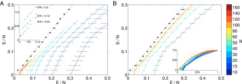
Entropy vs. energy. (A) Computed directly from the data. Different colors show results for different numbers of neurons; in each case, we choose 1,000 groups of size N at random, and points are means with SDs over groups. Inset shows extrapolations of the energy per neuron at fixed entropy per neuron, summarized as black points with error bars in the main plot. Dashed line is the best linear fit to the extrapolated points, . (B) Computed from the maximum entropy models. We choose neurons out of the population from which we record, and, for each of these subnetworks, we construct maximum entropy models as in Eq. 4; for details of the entropy calculation, see Supporting Information. Inset shows results for many subnetworks, and the main plot shows means and SDs across the different groups of N neurons. Black points with error bars are an extrapolation to infinite N, as in A, and the dashed line is .
As emphasized above, the plot of entropy vs. energy contains all of the thermodynamic behavior of a system, and this has a meaning for any probability distribution, even if we are not considering a system at thermal equilibrium. Thus, Fig. 3 is as close as we can get to constructing the thermodynamics of this network. With the direct counting of states, we see less and less of the plot at larger N, but the part we can see is approaching a limit as , and this is confirmed by the results from the maximum entropy models. This, by itself, is a significant result. If we write down a model like Eq. 4, then, in a purely theoretical discussion, we can scale the couplings between neurons with N to guarantee the existence of a thermodynamic limit (5), but with constructed from real data, we can’t impose this scaling ourselves—either it emerges from the data or it doesn’t. We can make the emergence of the thermodynamic limit more precise by noting that, at a fixed value of , the value of extrapolates to a well-defined limit in a plot vs. , as in Fig. 3A, Inset. The results of this extrapolation are strikingly simple: The entropy is equal to the energy, within (small) error bars.
Interpreting the Entropy vs. Energy Plot
If the plot of entropy vs. energy is a straight line with unit slope, then Eq. 2 is solved not by one single value of E but by a whole range. Not only do we have , as at an ordinary critical point, but all higher-order derivatives also are zero. Thus, the results in Fig. 3 suggest that the joint distribution of activity across neurons in this network is poised at a very unusual critical point.
We expect that states of lower probability (e.g., those in which more cells spike) are more numerous (because there are more ways to arrange K spikes among N cells as K increases from very low values). However, the usual result is that this trade-off—which is precisely the trade-off between energy and entropy in thermodynamics—selects typical states that all have roughly the same probability. The statement that , as suggested in Fig. 3, is the statement that states which are ten times less probable are exactly 10 times more numerous, and so there is no typical value of the probability.
The vanishing of corresponds, in an equilibrium system, to the divergence of the specific heat. Although the neurons obviously are not an equilibrium system, the model in Eqs. 3 and 4 is mathematically identical to the Boltzmann distribution. Thus, we can take this model seriously as a statistical mechanics problem, and compute the specific heat in the usual way. Further, we can change the effective temperature by considering a one-parameter family of models,
| [5] |
with as before (Eq. 4). Changing T is just a way of probing one direction in the parameter space of possible models, and is not a physical temperature; the goal is to see whether there is anything special about the model (at ) that describes the real system.
Results for the heat capacity of our model vs. T are shown in Fig. 4. There is a dramatic peak, and, as we look at larger groups of neurons, the peak grows and moves closer to , which is the model of the actual network. Importantly, the heat capacity grows even when we normalize by N, so that the specific heat, or heat capacity per neuron, is growing with N, as expected at a critical point, and these signatures are clearer in models that provide a more accurate description of the population activity; for details, see Supporting Information.
Fig. 4.

Heat capacity in maximum entropy models of neurons responding to naturalistic stimuli. (A) Heat capacity, , computed for subnetworks of neurons. Points are averages, and error bars are SDs, across 30 choices of subnetwork at each N. For details of the computations, see Supporting Information. (B) Zoom–in of the peak of , shown as an intensive quantity, . The peak moves toward with increasing N, and the growth of near is faster than linear with N. Green arrow points to results for a model of independent neurons whose spike probabilities (firing rates) match the data exactly; the heat capacity is exactly extensive.
The temperature is only one axis in parameter space, and, along this direction, there are variations in both the correlations among neurons and their mean spike rates. As an alternative, we consider a family of models in which the strength of correlations changes but spike rates are fixed. To do this, we replace the energy function in Eq. 4 with
| [6] |
where α controls the strength of correlations, and we adjust all of the to hold mean spike rates to their observed values.
At , the model describes a population of independent neurons, so that the correlation coefficients are all (Fig. 5A, Left). For , the distribution of correlations broadens such that at , some pairs are very strongly correlated (Fig. 5A, Right). This is reflected in a distribution of states that cluster around a small number of prototypical patterns, much as in the Hopfield network (4, 5). The entropy vs. energy plot, shown in Fig. 5B, singles out the ensemble at (Fig. 5A, Middle): Going toward independence (smaller α) gives rise to a concave bump at low energies, whereas ensembles deviate away from the equality line more at high energies. Correspondingly, we see in Fig. 5D that there is a peak in the specific heat of the model ensemble near . As we look at larger and larger networks, this peak rises and moves toward , which describes the real system.
Fig. 5.

Changing correlations at fixed spike rates. (A) Three maximum entropy (maxent) models for a 120-neuron network, where correlations have been eliminated (Left, ), left at the strength found in data (Middle, ), or scaled up (Right, ). (Top) The 10,000 most frequent patterns (black, spike; white, silence) in each model. (Bottom) The distribution of pairwise correlation coefficients. (B) Entropy vs. energy for the networks in A. (C) Entropy per neuron as a function of α, for different subnetwork sizes N. (D) Heat capacity per neuron exhibits a peak close to . Error bars are SDs over 10 subnetworks for each N and α.
The evidence for criticality that we find here is consistent with extrapolations from the analysis of smaller populations (15, 18). Those predictions were based on the assumption that spike probabilities and pairwise correlations in the smaller populations are drawn from the same distribution as in the full system, and that these distributions are sufficient to determine the thermodynamic behavior (36). Signs of criticality also are observable in simpler models, which match only the distribution of summed activity in the network (22), but less accurate models have weaker signatures of criticality (Fig. S2).
Couldn’t It Just Be…?
In equilibrium thermodynamics, poising a system at a critical point involves careful adjustment of temperature and other parameters. Finding that the retina seems to be poised near criticality should thus be treated with some skepticism. Here we consider some ways in which we could be misled into thinking that the system is critical when it is not (see also Supporting Information).
Part of our analysis is based on the use of maximum entropy models, and one could worry that the inference of these models is unreliable for finite data sets (37, 38). Expanding on the discussion of this problem in ref. 11, we find a clear peak in the specific heat when we learn models for neurons from even one-tenth of our data, and the variance across fractions of the data are only a few percent (Fig. S3).
Although the inference of maximum entropy models is accurate, less interesting models might mimic the signatures of criticality. In particular, it has been suggested that independent neurons with a broad distribution of spike rates could generate a distribution of N neuron activity patterns that mimics some aspects of critical behavior (39). However, in an independent model built from the actual spike rates of the neurons, the probability of seeing the same state twice would be less than one part in a billion, dramatically inconsistent with the measured . Such independent models also cannot account for the faster than linear growth of the heat capacity with N (Fig. 4), which is an essential feature of the data and its support for criticality.
In maximum entropy models, the probability distribution over patterns of neural activity is described in terms of interactions between neurons, such as the terms in Eq. 4; an alternative view is that the correlations result from the response of the neurons to fluctuating external signals. Testing this idea has a difficulty that has nothing to do with neurons: In equilibrium statistical mechanics, models in which spins (or other degrees of freedom) interact with one another are mathematically equivalent to a collection of spins responding independently to fluctuating fields (see Supporting Information for details). Thus, correlations always are interpretable as independent responses to unmeasured fluctuations, and, for neurons, there are many possibilities, including sensory inputs. However, the behavior that we see cannot be simply inherited from correlations in the visual stimulus, because we find signatures of criticality in response to movies with very different correlation structures (Fig. S4). Further, the pattern of correlations among neurons is not simply explained in terms of overlaps among receptive fields (Fig. S5), and, at fixed moments in the stimulus movie, neurons with nonzero spike probabilities have correlations across stimulus repetitions that can be even stronger than across the experiment as a whole (Fig. S6).
When we rewrite a model of interacting spins as independent spins responding to fluctuating fields, criticality usually requires that the distribution of fluctuations be very special, e.g., with the variance tuned to a particular value. In this sense, saying that correlations result from fluctuating inputs doesn’t explain our observations. Recently, it has been suggested that sufficiently broad distributions of fluctuations lead generically to critical phenomenology (40). As explained in Supporting Information, mean field models have the property that the variance of the effective fields becomes large at the critical point, but more general models do not, and the correlations we observe do not have the form expected from a mean field model. The fact that quantitative changes in the strength of correlations would drive the system away from criticality (Fig. 5D) suggests that the distribution of equivalent fluctuating fields must be tuned, rather than merely having sufficiently large fluctuations.
Discussion
The traditional formulation of the neural coding problem makes an analogy to a dictionary, asking for the meaning of each neural response in terms of events in the outside world (41). However, before we can build a dictionary, we need to know the lexicon, and, for large populations of neurons, this already is a difficult problem: With 160 neurons, the number of possible responses is larger than the number of words in the vocabulary of a well-educated English speaker, and is more comparable to the number of possible short phrases or sentences. In the same way that the distribution of letters in words embodies spelling rules (28), and the distribution of words in sentences encodes aspects of grammar (42) and semantic categories (43), we expect the distribution of activity across neurons to reveal structures of biological significance.
In the small patch of the retina that we consider, no two cells have truly identical input/output characteristics (44). Nonetheless, if we count how many combinations of spiking and silence have a given probability in groups of cells, this relationship is reproducible from group to group, and simplifies at larger N. This relationship between probability and numerosity of states is mathematically identical to the relationship between energy and entropy in statistical physics, and the simplification with increasing N suggests that we are seeing signs of a thermodynamic limit.
If we can identify the thermodynamic limit, we can try to place the network in a phase diagram of possible networks. Critical surfaces that separate different phases often are associated with a balance between probability and numerosity: States that are a factor F times less probable also are a factor F times more numerous. At conventional critical points, this balance occurs only in a small neighborhood of the typical probability, but, in the network of RGCs, it extends across a wide range of probabilities (Fig. 3). In model networks with slightly stronger or weaker correlations among pairs of neurons, this balance breaks down (Fig. 5), and less accurate models have weaker signatures of criticality (Fig. S2).
The strength of correlations depends on the structure of visual inputs, on the connectivity of the neural circuit, and on the state of adaptation in the system. The fact that we see signatures of criticality in response to very different movies, but not in model networks with stronger or weaker correlations, suggests that adaptation is tuning the system toward criticality. A sudden change of visual input statistics should thus drive the network to a noncritical state, and, during the course of adaptation, the distribution of activity should relax back to the critical surface. This can be tested directly.
Is criticality functional? The extreme inhomogeneity of the probability distribution over states makes it possible to have an instantaneously readable code for events that have a large dynamic range of likelihoods or surprise, and this may be well-suited to the the natural environment; it is not, however, an efficient code in the usual sense. Systems near critical points are maximally responsive to certain external signals, and this sensitivity also may be functionally useful. Most of the systems that exhibit criticality in the thermodynamic sense also exhibit a wide range of time scales in their dynamics, so that criticality may provide a general strategy for neural systems to bridge the gap between the microscopic time scale of spikes and the macroscopic time scales of behavior. Critical states are extremal in all these different senses, and more; it may be difficult to decide which is relevant for the organism.
Related signatures of criticality have been detected in ensembles of amino acid sequences for protein families (29), in flocks of birds (33) and swarms of insects (45), and in the network of genes controlling morphogenesis in the early fly embryo (46); there is also evidence that cell membranes have lipid compositions tuned to a true thermodynamic critical point (47). Different, dynamical notions of criticality have been explored in neural (48, 49) and genetic (50, 51) networks, and in the active mechanics of the inner ear (52–54); recent work connects dynamical and statistical criticality, with the retina as an example (55). These results hint at a general principle, but there is room for skepticism. A new generation of experiments should provide decisive tests of these ideas.
Materials and Methods
Experiments were performed on the larval tiger salamander, Ambystoma tigrinum tigrinum, in accordance with institutional animal care standards at Princeton University.
Supplementary Material
Acknowledgments
We thank A. Cavagna, D. S. Fisher, I. Giardina, M. Ioffe, S. C. F. van Opheusden, E. Schneidman, D. J. Schwab, J. P. Sethna, and A. M. Walczak for helpful discussions and comments on the manuscript. Research was supported in part by National Science Foundation Grants PHY-1305525, PHY-1451171, and CCF-0939370, by National Institutes of Health Grant R01 EY14196, and by Austrian Science Foundation Grant FWF P25651. Additional support was provided by the Fannie and John Hertz Foundation, by the Swartz Foundation, by the W. M. Keck Foundation, and by the Simons Foundation.
Footnotes
The authors declare no conflict of interest.
This article contains supporting information online at www.pnas.org/lookup/suppl/doi:10.1073/pnas.1514188112/-/DCSupplemental.
References
- 1.Anderson PW. More is different. Science. 1972;177(4047):393–396. doi: 10.1126/science.177.4047.393. [DOI] [PubMed] [Google Scholar]
- 2.Sethna JP. Statistical Mechanics: Entropy, Order Parameters, and Complexity. Oxford Univ Press; Oxford: 2006. [Google Scholar]
- 3.Guggenheim EA. The principle of corresponding states. J Chem Phys. 1945;13(7):253–261. [Google Scholar]
- 4.Hopfield JJ. Neural networks and physical systems with emergent collective computational abilities. Proc Natl Acad Sci USA. 1982;79(8):2554–2558. doi: 10.1073/pnas.79.8.2554. [DOI] [PMC free article] [PubMed] [Google Scholar]
- 5.Amit DJ. Modeling Brain Function: The World of Attractor Neural Networks. Cambridge Univ Press; Cambridge, UK: 1989. [Google Scholar]
- 6.Hertz J, Krogh A, Palmer RG. Introduction to the Theory of Neural Computation. Addison-Wesley; Redwood City, CA: 1991. [Google Scholar]
- 7.Ruelle D. Thermodynamic Formalism: The Mathematical Structures of Classical Equilibrium Statistical Mechanics. Addison-Wesley; Reading, MA: 1978. [Google Scholar]
- 8.Halsey TC, Jensen MH, Kadanoff LP, Procaccia I, Shraiman BI. Fractal measures and their singularities: The characterization of strange sets. Phys Rev A. 1986;33(2):1141–1151. doi: 10.1103/physreva.33.1141. [DOI] [PubMed] [Google Scholar]
- 9.Feigenbaum MJ, Jensen MH, Procaccia I. Time ordering and the thermodynamics of strange sets: Theory and experimental tests. Phys Rev Lett. 1986;57(13):1503–1506. doi: 10.1103/PhysRevLett.57.1503. [DOI] [PubMed] [Google Scholar]
- 10.Schnabel S, Seaton DT, Landau DP, Bachmann M. Microcanonical entropy inflection points: Key to systematic understanding of transitions in finite systems. Phys Rev E Stat Nonlin Soft Matter Phys. 2011;84(1 Pt 1):011127. doi: 10.1103/PhysRevE.84.011127. [DOI] [PubMed] [Google Scholar]
- 11.Tkačik G, et al. Searching for collective behavior in a large network of sensory neurons. PLoS Comput Biol. 2014;10(1):e1003408. doi: 10.1371/journal.pcbi.1003408. [DOI] [PMC free article] [PubMed] [Google Scholar]
- 12.Marre O, et al. Mapping a complete neural population in the retina. J Neurosci. 2012;32(43):14859–14873. doi: 10.1523/JNEUROSCI.0723-12.2012. [DOI] [PMC free article] [PubMed] [Google Scholar]
- 13.Jaynes ET. Information theory and statistical mechanics. Phys Rev. 1957;106(4):620–630. [Google Scholar]
- 14.Schneidman E, Berry MJ, 2nd, Segev R, Bialek W. Weak pairwise correlations imply strongly correlated network states in a neural population. Nature. 2006;440(7087):1007–1012. doi: 10.1038/nature04701. [DOI] [PMC free article] [PubMed] [Google Scholar]
- 15.Tkačik G, Schneidman E, Berry MJ, II, Bialek W. 2006. Ising models for networks of real neurons. arXiv:q-bio/0611072.
- 16.Shlens J, et al. The structure of multi-neuron firing patterns in primate retina. J Neurosci. 2006;26(32):8254–8266. doi: 10.1523/JNEUROSCI.1282-06.2006. [DOI] [PMC free article] [PubMed] [Google Scholar]
- 17.Tang A, et al. A maximum entropy model applied to spatial and temporal correlations from cortical networks in vitro. J Neurosci. 2008;28(2):505–518. doi: 10.1523/JNEUROSCI.3359-07.2008. [DOI] [PMC free article] [PubMed] [Google Scholar]
- 18.Tkačik G, Schneidman E, Berry MJ, II, Bialek W. 2009. Spin glass models for a network of real neurons. arXiv:0912.5409.
- 19.Shlens J, et al. The structure of large-scale synchronized firing in primate retina. J Neurosci. 2009;29(15):5022–5031. doi: 10.1523/JNEUROSCI.5187-08.2009. [DOI] [PMC free article] [PubMed] [Google Scholar]
- 20.Ohiorhenuan IE, et al. Sparse coding and high-order correlations in fine-scale cortical networks. Nature. 2010;466(7306):617–621. doi: 10.1038/nature09178. [DOI] [PMC free article] [PubMed] [Google Scholar]
- 21.Ganmor E, Segev R, Schneidman E. Sparse low-order interaction network underlies a highly correlated and learnable neural population code. Proc Natl Acad Sci USA. 2011;108(23):9679–9684. doi: 10.1073/pnas.1019641108. [DOI] [PMC free article] [PubMed] [Google Scholar]
- 22.Tkačik G, et al. The simplest maximum entropy model for collective behavior in a neural network. J Stat Mech. 2013;2013:P03011. [Google Scholar]
- 23.Granot-Atedgi E, Tkačik G, Segev R, Schneidman E. Stimulus-dependent maximum entropy models of neural population codes. PLOS Comput Biol. 2013;9(3):e1002922. doi: 10.1371/journal.pcbi.1002922. [DOI] [PMC free article] [PubMed] [Google Scholar]
- 24.Lezon TR, Banavar JR, Cieplak M, Maritan A, Fedoroff NV. Using the principle of entropy maximization to infer genetic interaction networks from gene expression patterns. Proc Natl Acad Sci USA. 2006;103(50):19033–19038. doi: 10.1073/pnas.0609152103. [DOI] [PMC free article] [PubMed] [Google Scholar]
- 25.Tkačik G. 2007. Information flow in biological networks. dissertation (Princeton University, Princeton, NJ)
- 26.Bialek W, Ranganathan R. 2007. Rediscovering the power of pairwise interactions. arXiv:0712.4397.
- 27.Weigt M, White RA, Szurmant H, Hoch JA, Hwa T. Identification of direct residue contacts in protein−protein interaction by message passing. Proc Natl Acad Sci USA. 2009;106(1):67–72. doi: 10.1073/pnas.0805923106. [DOI] [PMC free article] [PubMed] [Google Scholar]
- 28.Stephens GJ, Bialek W. Statistical mechanics of letters in words. Phys Rev E Stat Nonlin Soft Matter Phys. 2010;81(6 Pt 2):066119. doi: 10.1103/PhysRevE.81.066119. [DOI] [PMC free article] [PubMed] [Google Scholar]
- 29.Mora T, Walczak AM, Bialek W, Callan CG., Jr Maximum entropy models for antibody diversity. Proc Natl Acad Sci USA. 2010;107(12):5405–5410. doi: 10.1073/pnas.1001705107. [DOI] [PMC free article] [PubMed] [Google Scholar]
- 30.Marks DS, et al. Protein 3D structure computed from evolutionary sequence variation. PLoS One. 2011;6(12):e28766. doi: 10.1371/journal.pone.0028766. [DOI] [PMC free article] [PubMed] [Google Scholar]
- 31.Sułkowska JI, Morcos F, Weigt M, Hwa T, Onuchic JN. Genomics-aided structure prediction. Proc Natl Acad Sci USA. 2012;109(26):10340–10345. doi: 10.1073/pnas.1207864109. [DOI] [PMC free article] [PubMed] [Google Scholar]
- 32.Bialek W, et al. Statistical mechanics for natural flocks of birds. Proc Natl Acad Sci USA. 2012;109(13):4786–4791. doi: 10.1073/pnas.1118633109. [DOI] [PMC free article] [PubMed] [Google Scholar]
- 33.Bialek W, et al. Social interactions dominate speed control in poising natural flocks near criticality. Proc Natl Acad Sci USA. 2014;111(20):7212–7217. doi: 10.1073/pnas.1324045111. [DOI] [PMC free article] [PubMed] [Google Scholar]
- 34.Santolini M, Mora T, Hakim V. A general pairwise interaction model provides an accurate description of in vivo transcription factor binding sites. PLoS One. 2014;9(6):e99015. doi: 10.1371/journal.pone.0099015. [DOI] [PMC free article] [PubMed] [Google Scholar]
- 35.Mora T, Bialek W. Are biological systems poised at criticality? J Stat Phys. 2011;144(2):268–302. [Google Scholar]
- 36.Castellana M, Bialek W. Inverse spin glass and related maximum entropy problems. Phys Rev Lett. 2014;113(11):117204. doi: 10.1103/PhysRevLett.113.117204. [DOI] [PubMed] [Google Scholar]
- 37.Mastromatteo I, Marsili M. On the criticality of inferred models. J Stat Mech. 2011;2011:P10012. [Google Scholar]
- 38.Marsili M, Mastromatteo I, Roudi Y. On sampling and modeling complex systems. J Stat Mech. 2013;2013:P09003. [Google Scholar]
- 39.van Opheusden SCF. 2013. Critical states in retinal population codes, Masters thesis (Universiteit Leiden, Leiden, The Netherlands)
- 40.Schwab DJ, Nemenman I, Mehta P. Zipf’s law and criticality in multivariate data without fine-tuning. Phys Rev Lett. 2014;113(6):068102. doi: 10.1103/PhysRevLett.113.068102. [DOI] [PMC free article] [PubMed] [Google Scholar]
- 41.Rieke F, Warland D, de Ruyter van Steveninck R, Bialek Spikes W. Exploring the Neural Code. MIT Press; Cambridge, MA: 1997. [Google Scholar]
- 42.Pereira F. Formal grammar and information theory: Together again? Philos Trans R Soc Lond A. 2000;358:1239–1253. [Google Scholar]
- 43.Pereira FC, Tishby N, Lee L. 1993. Distributional clustering of English words. Proceedings of the 31st Annual Meeting of the Association for Computational Linguistics, ed Schubert LK (Assoc Comput Linguist, Stroudsburg, PA), pp 183–190.
- 44.Schneidman E, Bialek W, Berry MJ., II . An information theoretic approach to the functional classification of neurons. In: Becker S, Thrun S, Obermayer K, editors. Advances in Neural Information Processing 15. MIT Press; Cambridge, MA: 2003. pp. 197–204. [Google Scholar]
- 45.Attanasi A, et al. Finite-size scaling as a way to probe near-criticality in natural swarms. Phys Rev Lett. 2014;113(23):238102. doi: 10.1103/PhysRevLett.113.238102. [DOI] [PubMed] [Google Scholar]
- 46.Krotov D, Dubuis JO, Gregor T, Bialek W. Morphogenesis at criticality. Proc Natl Acad Sci USA. 2014;111(10):3683–3688. doi: 10.1073/pnas.1324186111. [DOI] [PMC free article] [PubMed] [Google Scholar]
- 47.Honerkamp-Smith AR, Veatch SL, Keller SL. An introduction to critical points for biophysicists; observations of compositional heterogeneity in lipid membranes. Biochim Biophys Acta. 2009;1788(1):53–63. doi: 10.1016/j.bbamem.2008.09.010. [DOI] [PMC free article] [PubMed] [Google Scholar]
- 48.Beggs JM, Plenz D. Neuronal avalanches in neocortical circuits. J Neurosci. 2003;23(35):11167–11177. doi: 10.1523/JNEUROSCI.23-35-11167.2003. [DOI] [PMC free article] [PubMed] [Google Scholar]
- 49.Friedman N, et al. Universal critical dynamics in high resolution neuronal avalanche data. Phys Rev Lett. 2012;108(20):208102. doi: 10.1103/PhysRevLett.108.208102. [DOI] [PubMed] [Google Scholar]
- 50.Nykter M, et al. Gene expression dynamics in the macrophage exhibit criticality. Proc Natl Acad Sci USA. 2008;105(6):1897–1900. doi: 10.1073/pnas.0711525105. [DOI] [PMC free article] [PubMed] [Google Scholar]
- 51.Balleza E, et al. Critical dynamics in genetic regulatory networks: Examples from four kingdoms. PLoS One. 2008;3(6):e2456. doi: 10.1371/journal.pone.0002456. [DOI] [PMC free article] [PubMed] [Google Scholar]
- 52.Eguíluz VM, Ospeck M, Choe Y, Hudspeth AJ, Magnasco MO. Essential nonlinearities in hearing. Phys Rev Lett. 2000;84(22):5232–5235. doi: 10.1103/PhysRevLett.84.5232. [DOI] [PubMed] [Google Scholar]
- 53.Camalet S, Duke T, Jülicher F, Prost J. Auditory sensitivity provided by self-tuned critical oscillations of hair cells. Proc Natl Acad Sci USA. 2000;97(7):3183–3188. doi: 10.1073/pnas.97.7.3183. [DOI] [PMC free article] [PubMed] [Google Scholar]
- 54.Ospeck M, Eguíluz VM, Magnasco MO. Evidence of a Hopf bifurcation in frog hair cells. Biophys J. 2001;80(6):2597–2607. doi: 10.1016/S0006-3495(01)76230-3. [DOI] [PMC free article] [PubMed] [Google Scholar]
- 55.Mora T, Deny S, Marre O. Dynamical criticality in the collective activity of a population of retinal neurons. Phys Rev Lett. 2015;114(7):078105. doi: 10.1103/PhysRevLett.114.078105. [DOI] [PubMed] [Google Scholar]
Associated Data
This section collects any data citations, data availability statements, or supplementary materials included in this article.