Reducing sensitivity losses due to respiration and motion in accelerated Echo Planar Imaging by reordering the auto-calibration data acquisition

Abstract

Purpose

To reduce the sensitivity of echo-planar imaging (EPI) Auto-Calibration Signal (ACS) data to patient respiration and motion in order to improve the image quality and temporal Signal-to-Noise Ratio (tSNR) of accelerated EPI time-series data.

Methods

ACS data for accelerated EPI are generally acquired using segmented, multi-shot EPI to distortion-match the ACS and time-series data. The ACS data are therefore typically collected over multiple TR periods, leading to increased vulnerability to motion and dynamic B₀ changes. The Fast Low-angle Excitation Echo-planar Technique (FLEET) is adopted to reorder the ACS segments so that segments within any given slice are acquired consecutively in time, thereby acquiring ACS data for each slice as rapidly as possible.

Results

Subject breath-hold and motion phantom experiments demonstrate that artifacts in the ACS data reduce tSNR and produce tSNR discontinuities across slices in the accelerated EPI time-series data. Accelerated EPI data reconstructed using FLEET-ACS exhibit improved tSNR and increased tSNR continuity across slices. Additionally, image quality is improved dramatically when bulk motion occurs during the ACS acquisition.

Conclusion

FLEET-ACS provides reduced respiration and motion sensitivity in accelerated EPI, which yields higher tSNR and image quality. Benefits are demonstrated in both conventional-resolution 3T and high-resolution 7T EPI time-series data.

INTRODUCTION

Echo-Planar Imaging (EPI) is a commonly-used method for rapid MRI and the main imaging technique used for functional, diffusion and perfusion MRI. Accelerated parallel imaging can reduce the number of phase-encoding steps, thereby reducing total readout time and effective echo-spacing. These reductions decrease image blur and geometric distortion caused by off-resonance effects (1). Therefore accelerated EPI is a critical tool for high-resolution and ultrahigh-field applications. The GeneRalized Autocalibrating Partially Parallel Acquisitions (GRAPPA) parallel imaging method (2) is often used for the image reconstruction due to its use of Auto-Calibration Signal (ACS) data rather than explicitly estimated coil sensitivity profiles. Multiple EPI measurements are generally required in functional, diffusion, and perfusion imaging, and therefore the ACS data can consist of a single, Nyquist-sampled dataset acquired at the beginning of each run, followed by the repeated acquisition of undersampled EPI data.

Although GRAPPA is somewhat insensitive to the image contrast of the ACS data (3), the training data should have the same k-space sampling parameters as the accelerated data. This will not be the case in the presence of susceptibility gradients unless the ACS data are acquired with the same velocity in k-space as the accelerated data, i.e., the effective echo-spacing of the two acquisitions must be matched. The simplest approach is to acquire the fully-sampled ACS data as segmented EPI with the number of segments equaling the acceleration factor R. Then, any geometric distortions in the image data are also present in the ACS data (4). To allow for longitudinal magnetization recovery between shots in multiple-slice acquisitions, the segmented ACS data are routinely acquired in an efficient, “consecutive-slice” manner in which the first segment is acquired across all slices, then the second segment across all slices, and so on. In this way, the inner loop of the acquisition traverses the slices and the outer loop traverses the segments; the time interval between the first and last segments for a given slice is then (R–1)·TR, where R is both the acceleration factor and the number of segments. This interval can be between 2 and 10 s for standard imaging protocols.

A major drawback of this approach is that if the (R–1)·TR interval becomes more than ~1 s, the ACS segments will likely be collected at different phases of the respiratory cycle. Because respiration induces spatially non-uniform B₀ offsets, this can lead to differing phase shifts of each ACS segment. Lengthy inter-segment acquisition times also increase the chance for patient movement during this critical component of the acquisition. The resulting artifactual discontinuities across ACS segments will influence the GRAPPA kernel training, and the resulting kernel will then propagate artifacts and noise into the final accelerated image reconstruction. Thus, depending on the timing of the ACS data and its relation to the patient motion or breathing, the artifact and noise levels may vary substantially from slice to slice—since any given slice of ACS data may be acquired at a variety of head positions or phases in the respiratory cycle.

An example of how signal-to-noise ratio (SNR) can be influenced by acquisition timing for a typical interleaved-slice acquisition is shown in Fig. 1; note that the errors in the GRAPPA kernel affect both image SNR (SNR₀) and time-series SNR (tSNR), as demonstrated in this example. The reduced SNR seen in a subset (roughly half) of the slices not only hampers the detection of fMRI activation within those slices but the resulting discontinuous SNR in this slice-interleaved acquisition represents a spatial bias in functional, diffusion, or perfusion MRI studies. In fMRI, tSNR is related to functional Contrast-to-Noise Ratio (fCNR) via the relationship fCNR = (ΔS/S)·tSNR (5), where ΔS/S represents percent fMRI signal change which is determined by the neuronal and hemodynamic responses to the stimulus or task; thus tSNR is the central experimental factor that determines the statistical significance of an fMRI activation. Therefore for fMRI studies of focal activation patterns this discontinuous tSNR could lead to more frequent false negatives and loss of statistical significance within the low-SNR slices, especially for studies where sensitivity is limited (such as studies involving subtle cognitive tasks or studies using high-resolution acquisitions). A changing pattern of discontinuous tSNR across slices would introduce a new source of variability when combining data across both runs and subjects. Also, spatially smoothing data with discontinuous tSNR across slices could cause spatial shift in the loci of activation. In diffusion imaging, the discontinuous image SNR can reduce the accuracy of tensor fitting in a subset of slices, adding variability to fractional anisotropy maps and complicating tractography. If instead a non-interleaved (i.e., a “sequential”, either ascending or descending) slice ordering is used, reduced SNR would still be present but less apparent—a spatially continuous SNR would result but a systematic relationship between slice position and SNR level would still occur.

Fig. 1.

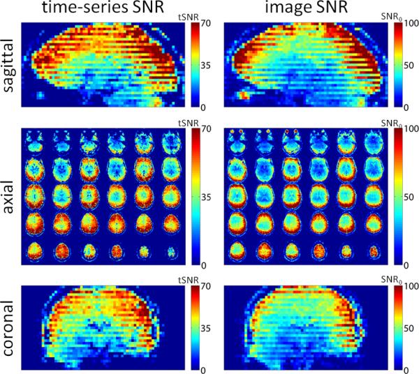
Effects of ACS acquisition on SNR of EPI data. SNR maps of conventional single-shot EPI (3×3×3 mm³, 32-channel RF coil array, BOLD-weighted, 3T) with R=3 acceleration, are shown both in a native axial mosaic as well as coronal and sagittal reformats. The EPI time-series data were reconstructed with GRAPPA using kernels derived from an echo-spacing-matched multi-shot (N_s=3) ACS acquisition. The resulting tSNR and image SNR from the resulting images are shown. Both tSNR and image SNR exhibit SNR discontinuities across slices in the images reconstructed with a kernel derived from multi-shot EPI ACS data.

One potential solution is to replace the EPI acquisition of ACS data with another rapid acquisition, such as Fast Low-Angle SHot (FLASH) imaging (6), which does not suffer from the same sensitivity to dynamic B₀ effects and Nyquist ghosting. FLASH-ACS data have been used to reconstruct accelerated EPI data with GRAPPA (3,7) with improved SNR in the reconstructed EPI time-series (7). However this method also suffers from an echo-spacing mismatch and consequently differential geometric distortion between the ACS data and the accelerated EPI data, limiting its utility to cases where susceptibility distortion in the EPI data is minimal. It may be possible to account for these differential distortions by estimating a B₀ map during the imaging session and removing the mismatch (8–10), but this approach necessitates acquiring a B₀ map, is vulnerable to errors caused by patient movement between the B₀ map and EPI acquisitions, and somewhat defeats the purpose of having an auto-calibrated reconstruction. Therefore a method for acquiring ACS data with matched geometric distortion is desired.

The conventional time-ordering of the segments in a multi-shot EPI-based ACS acquisition maximizes the time interval between the acquisitions of the segments in each slice. While this is favorable from a magnetization recovery point-of-view, it is unfavorable from motion or respiratory phase sensitivity points-of-view. It is, however, possible to reorder the acquisition to minimize the time interval between segments, such that all segments within a slice are acquired consecutively before acquiring another slice, with a cost in available longitudinal magnetization and (potentially) a small increase in acquisition time. For a given tissue T₁ and recovery time between shots, a simple flip-angle progression can be calculated to ensure that equal magnetization is available for each segment (11). This “consecutive-segment” multi-shot EPI has been explored for high-resolution functional imaging (12–14). In cases where many T₁ values are present in the slice, this flip-angle progression can be replaced by repeating the same low flip angle for each segment, which reduces the dependence on a specific T₁ value. The latter technique—a hybrid of segmented EPI and FLASH—is known as Fast Low-angle Excitation Echo-planar Technique (FLEET) (15).

Here we propose to use a consecutive-segment multi-shot EPI-based ACS acquisition to reduce motion and respiratory-cycle effects on the time-series data. We analyze two variants: using a progression of flip angles that uses all of the available magnetization while maintaining the signal level across segments; and using a constant, low flip angle, which yields roughly equal signal levels across segments but utilizes a fraction of the available magnetization. Both strategies re-order the segments so that a given slice's segments are acquired with the minimum time separation. This separation is approximately the duration needed to excite and encode a single EPI segment, which for a conventional single-shot acquisition is approximately τ=TR/N_slice or ~65 ms for typical 2-mm isotropic, R=2, whole-brain 3T fMRI protocols. By shortening the period within the ACS acquisition that is vulnerable to motion and respiration from (R-1)·TR to τ (a shortening factor of (R-1)·N_slice, which is over 50 for whole-brain 2 mm protocols) we show a greatly reduced sensitivity to patient-driven changes occurring during the ACS acquisition. Since the effective echo-spacing of the ACS matches that of the accelerated readout (for matched geometric distortion), the approach does not suffer from secondary GRAPPA artifacts—which are expected for other fast ACS approaches such as FLASH-ACS.

We show that this alternative to conventional consecutive-slice multi-shot EPI leads to reduced artifacts due to overt motion, increased SNR in the EPI time-series data, and smooth SNR across slices. Because of the increased severity of both static and dynamic B₀ changes at ultrahigh-field strengths, we evaluated its performance at both 3T and 7T. A preliminary account of this study has been presented in abstract form (16).

METHODS

Participants

Fourteen healthy adults (six female) volunteered to participate in the study (ages 21–52, mean 30.2 ± 9.4 s.d.). Written informed consent was obtained from each participant prior to the experiment in accordance with our institution's Human Research Committee. Four subjects participated in initial 3T scanning, five more participated in separate 3T breath-hold tests (described below), and five additional subjects participated in 7T scanning. All subjects were instructed to remain still throughout the scanning.

Pulse sequences

In R-fold undersampled EPI, the number of segments in the multi-shot ACS acquisition, N_s, is generally equal to the acceleration factor (i.e., R=N_s) in order to acquire Nyquist-sampled data whose echo-spacing is matched to the effective echo-spacing of the accelerated data. We refer to the conventional segmented, multi-shot EPI as “consecutive-slice” segmented EPI (see Fig. 2A). An alternative segmented EPI scheme is depicted in Fig. 2B (henceforth referred to as “consecutive-segment” imaging). In this alternate scheme, the loop-order of the segments and slices is swapped. In “consecutive-segment” ordering the time interval between the acquisitions of adjacent segments within a slice is minimized and is equivalent to the recovery time, τ. This reduces the time available for longitudinal magnetization recovery, since now τ<TR, which reduces the overall signal level and therefore the flip angles must be chosen so that each segment has equal magnetization. Thus there are two approaches to setting the flip angles across segments: either calculate the progression that maximizes and equalizes the magnetization (e.g., for a three-segment slice and $\tau \ll {\mathsf{T}}_1$ the flip angles are: 35.3°–45°–90°); or use the same low flip angle for each segment (e.g., 20°) which requires preparation RF pulses before the acquisition to bring the magnetization into steady state. This first approach with a variable flip angle, developed by Mansfield (11) has been referred to as interleaved snapshot EPI (12), consecutive-interleaved EPI (13), and turbo-segmented EPI (14); here we refer to this method as Variable Flip-Angle (VFA) FLEET. The second “consecutive-segment” approach that uses a constant flip angle is generally known as FLEET (15), which is a special case of FLEET-VFA.

Fig. 2.

Schematics of ACS data acquisition approaches. (A) Acquisition order of k-space segments from an example consecutive-slice multi-shot EPI protocol with 2 segments and 3 slices, comprising conventional ACS data for R=2 accelerated EPI. Each panel depicts a time step of the acquisition, and the acquisition progresses from left to right. (Thick black traces denote k-space lines acquired at each time point t, dashed blue lines denote missing k-space lines, solid purple lines denote acquired k-space lines.) Readout and phase-encode directions are indicated in first panel. (B) Acquisition order from the corresponding consecutive-segment multi-shot EPI protocol. In this ordering scheme, all segments from Slice 1 are acquired before progressing to acquire data in Slice 2, minimizing the time interval between the acquisitions of all segments within a particular slice. (C) Pulse sequence block diagram depicting the acquisition of a single slice in the proposed consecutive-segment acquisition, including fat saturation and gradient spoiling modules. (We define the duration per slice as the time required for all components within the dashed border; see Table 1.) (D) Full pulse sequence diagram, including the acquisition modules with dashed borders representing the sequence block from (C), followed by the accelerated image acquisition.

A schematic of the pulse sequence proposed here for a single slice in the FLEET or FLEET-VFA consecutive-segment schemes is presented in Fig. 2C. The module consists of two stages. First, an optional series of preparation RF pulses may be required to establish steady-state magnetization for the segments; in this case the module begins with N_d preparation segments. Second, the ACS data are acquired across all N_s segments. RF and gradient spoiling are employed to help eliminate remaining transverse magnetization; RF spoiling phase increment was set to 117° (17), the gradient moments were fully rewound before gradient spoiling, and the gradient spoiler moment was set to produce a 10π dephasing for a 10 mm reference pixel. Echo shifting is employed between segments (18–21) to ensure a consistent phase evolution and T₂* decay over the segments. Because the image contrast in the ACS data is not required to match that of the accelerated data, TE is minimized in the ACS acquisition to shorten acquisition time. Fat saturation pulses are played out only before the first shot of each slice because fat signal is not expected to fully recover during the typically short duration of the FLEET acquisition.

The full sequence diagram is presented in Fig. 2D. ACS data are acquired first, followed immediately by an optional series of N_D image dummy acquisitions included to establish a new steady-state magnetization for the image acquisitions—because the flip angle and the recovery time will differ between the ACS and accelerated image data, these dummy scans are required to avoid transients in magnetization that would occur when switching between these two steady states.

FLEET and FLEET-VFA both attempt to provide a constant longitudinal magnetization across segments. FLEET-VFA uses the full magnetization available, and the flip angle evolution can be calculated from the Bloch equations given the recovery time τ assuming a fixed T₁ value (11,15,21); the expression is provided in the Supporting Methods. However, because there are many T₁ values present in the head, unwanted differences in magnetization levels across segments may ensue, causing artifacts. To combat this, FLEET employs a constant, small flip angle for each shot. In this case, the shots modulate the magnetization only by a small amount and thus the signal levels across segment are approximately equal even in the presence of a moderate range of T₁ values, however each segment utilizes a small fraction of the available magnetization (see Supporting Fig. 1). A potential drawback of the FLEET approach is the transient in longitudinal magnetization level that occurs during the first few segments in the approach towards steady state. This is partially addressed by the preparation RF pulses prior to the first segment (21); however if a small enough constant flip angle is used even though the magnetization will not reach a proper steady state the change in signal levels across segments will be minor enough that preparation pulses may not be necessary. In this study cases both with and without preparation pulses are tested. The choice of constant flip angle must balance maximizing signal level with providing uniform-enough levels across segments so as to not interfere with the GRAPPA training, and so we empirically determined several flip angles that work well in practice.

Data Acquisition

The 3T data were acquired on a MAGNETOM Trio, a Tim System 3T whole-body scanner (Siemens AG, Healthcare Sector, Erlangen, Germany) running pulse sequence and image reconstruction software version VB17A Service Pack 4 using the manufacturer's 32-channel coil. We used the manufacturer's prototype implementation of an EPI pulse sequence with single-shot ACS, conventional consecutive-slice ACS, and FLASH-ACS (WIP #676b) and our custom implementation of the FLEET-ACS integrated into the standard EPI pulse sequence. All 3T data were acquired using a typical, accelerated single-shot gradient-echo EPI protocol with nominal 3×3 mm² in-plane voxel size, TE/TR/BW/matrix/flip angle=30 ms/2000 ms/2368 Hz/pix/96×96/90°, a nominal echo-spacing of 0.51 ms, 29 slice-interleaved, 3-mm thick axial slices (no gap), and 100 time points. The duration of the ACS scan varied across the different schemes employed. A large field-of-view was chosen in order to facilitate quantification of residual aliasing and ghost artifacts in the reconstructed images.

Acceleration factors R=2, 3, and 4 were tested, and for each protocol the maximum number of reference lines was acquired. In the FLEET-VFA protocols the flip angles were (after integer rounding): 45°-90° for R=2; 35°-45°-90° for R=3; 30°-35°-45°-90° for R=4 (11,21). We also tested ACS acquisitions based on FLEET with α_i=5° (which we denote as “FLEET5”) and α_i=20° (“FLEET20”). In the FLEET20 scheme we added five preparation RF pulses (i.e., N_d=5). For all consecutive-segment acquisitions four image dummy pulses were played between the ACS and image acquisitions (i.e., N_D=4) to match the number typically used in fMRI protocols with a TR of 2 s and a flip angle near 90°.

Conventional consecutive-slice multi-shot EPI ACS data, single-shot EPI ACS data (with a reduced number of reference lines and an echo-spacing set to the nominal echo-spacing of the accelerated acquisition), and 2D multi-slice FLASH-ACS data were acquired using the prototype sequence. The FLASH-ACS acquisition was not slice-interleaved, therefore, like the FLEET acquisition, the k-space data for each slice were fully acquired before beginning the acquisition of the next slice. See Table 1A for details of the 3T protocols tested. We also acquired data using all protocols on a 17-cm spherical phantom filled with agar gel (T₁≈400 ms at 3T) fabricated by the Biomedical Informatics Research Network (http://www.birncommunity.org/).

Table 1.

Detailed list of EPI protocol parameters.

method	R	voxel size (mm)	matrix	slice thick (mm)	no. of slices	TR (s)	TE (ms)	p.F.	f.a.	BW (Hz/pix)	esp. (ms)	ACS lines	ACS f.a.	ACS TE (ms)	ACS BW (Hz/pix)	ACS dummies	duration/ slice (ms)
(A) 3 T protocols
conv.	2	3	96	3	29	2	30	off	90°	2368	0.51	94	90°	30	-	-	138
single-shot	2	3	96	3	29	2	30	off	90°	2368	0.51	48	90°	30	-	-	69
FLASH	2	3	96	3	29	2	30	off	90°	2368	0.51	96	5°	4.8	1000	-	595
FLEET5	2	3	96	3	29	2	30	off	90°	2368	0.51	94	5°	16.4	-	0	80
FLEET20	2	3	96	3	29	2	30	off	90°	2368	0.51	94	20°	16.4	-	5	246
FLEET-VFA	2	3	96	3	29	2	30	off	90°	2368	0.51	94	45°-90°	16.4	-	0	80
conv.	3	3	96	3	29	2	30	off	90°	2368	0.51	90	90°	30	-	-	207
single-shot	3	3	96	3	29	2	30	off	90°	2368	0.51	30	90°	30	-	-	69
FLASH	3	3	96	3	29	2	30	off	90°	2368	0.51	90	5°	4.8	1000	-	559
FLEET5	3	3	96	3	29	2	30	off	90°	2368	0.51	90	5°	12.1	-	0	86
FLEET20	3	3	96	3	29	2	30	off	90°	2368	0.51	90	20°	12.1	-	5	209
FLEET-VFA	3	3	96	3	29	2	30	off	90°	2368	0.51	90	35°-45°-90°	12.1	-	0	86
conv.	4	3	96	3	29	2	30	off	90°	2368	0.51	88	90°	30	-	-	276
single-shot	4	3	96	3	29	2	30	off	90°	2368	0.51	24	90°	30	-	-	69
FLASH	4	3	96	3	29	2	30	off	90°	2368	0.51	88	5°	4.8	1000	-	546
FLEET5	4	3	96	3	29	2	30	off	90°	2368	0.51	76	5°	9.6	-	0	91
FLEET20	4	3	96	3	29	2	30	off	90°	2368	0.51	76	20°	9.6	-	5	187
FLEET-VFA	4	3	96	3	29	2	30	off	90°	2368	0.51	76	30°-35°-45°-90°	9.6	-	0	91
(B) 7 T protocols
conv.	3	3.0	96	3.0	28	2	20	off	80°	2368	0.53	90	80°	20	-	-	214
FLASH	3	3.0	96	3.0	28	2	20	off	80°	2368	0.53	90	5°	4.8	1000	-	622
FLEET	3	3.0	96	3.0	28	2	20	off	80°	2368	0.53	90	20°	12.2	-	10	325
conv.	3	1.5	128	1.5	37	2	25	off	67°	1776	0.67	126	67°	25	-	-	162
FLASH	3	1.5	128	1.5	37	2	25	off	67°	1776	0.67	126	5°	3.2	1000	-	620
FLEET	3	1.5	128	1.5	37	2	25	off	67°	1776	0.67	126	20°	19.5	-	6	364
conv.	4	1.0	192	1.0	46	3	27	7/8	90°	1184	1.00	128	90°	27	-	-	261
FLASH	4	1.0	192	1.0	46	3	27	7/8	90°	1184	1.00	128	5°	3.2	1000	-	625
FLEET	4	1.0	192	1.0	46	3	27	7/8	90°	1184	1.00	128	10°	24.5	-	3	321

(A) 3T protocols. All 3T protocols had common parameter values for the accelerated image acquisition. (B) 7T protocols. Three basic protocols were used, and for each protocol three variants of ACS data acquisition were tested. (Note that duration per slice is defined here as the total ACS acquisition time per slice, which for conventional consecutive-slice acquisitions is a function of TR and the number of slices. For the conventional consecutive-slice ACS acquisitions the ACS flip angle was identical to the accelerated acquisition flip angle. p.F. = partial Fourier factor; f.a.= flip angle; esp. = nominal echo-spacing.)

The 7T data were acquired on a research whole-body system (Siemens AG, Erlangen, Germany) running pulse sequence and image reconstruction software version VB17A UHF and equipped with body gradients using a custom-made 32-channel coil and birdcage volume coil for transmit (22). In the 7T sessions we tested 3×3×3 mm³ voxel size protocols with R=3 (to compare with the 3T data), 1.5×1.5×1.5 mm³ voxel size protocols with R=3 and 1.0×1.0×1.0 mm³ voxel size protocols with R=4. Because of the longer T₁ values at 7T, for the highest-resolution protocol we chose a FLEET flip angle somewhat larger than 5° to provide increased signal level; we tested a FLEET protocol with α_i =10°, denoted “FLEET10”. We did not attempt a single-shot ACS acquisition or a FLEET-VFA acquisition at 7T. See Table 1B for full details of all 7T protocols.

Deliberate shim offset tests

To assess the impact of susceptibility distortion, additional scans were acquired during the 3T sessions where B₀ inhomogeneity was induced by manually offsetting the linear x gradient offset “shim” by 50 μT/m causing a range of B₀ offsets between about ±150 Hz within the brain, similar to the offsets expected near air-tissue interfaces at 3T (8), which was enough to cause noticeable distortion in the unaccelerated images while causing acceptable distortion in the accelerated images (see Fig. 5). The resulting differences in ghost levels were quantified from a Region of Interest (ROI) outside of the brain (see Supporting Methods).

Fig. 5.

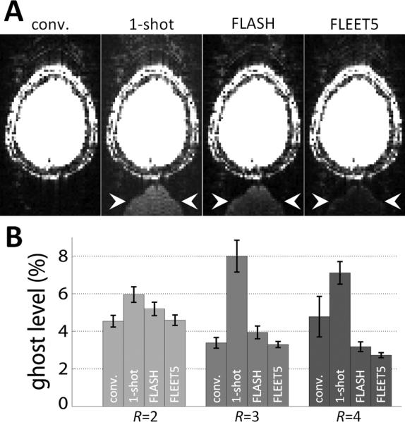
Dependence of residual aliasing on B₀ effects. (A) Example images from R=3 accelerated images reconstructed using consecutive-slice ACS, single-shot EPI ACS (“1-shot”), FLASH-ACS, and FLEET5-ACS data from a 3T subject in the presence of a small, intentional shim offset to provoke differential distortion between the ACS data and the accelerated data. The pattern of the ghost in these examples is quite typical: a low ghost level is seen in the images reconstructed from the conventional consecutive-slice ACS data, while strong ghosting is seen when using the single-shot ACS data, and the ghosts seen when using FLASH-ACS data are prominent and spatially flat, whereas the ghosts seen when using the FLEET-ACS data are still visible but consist of a high-spatial-frequency edge artifact (ghost locations by arrowhead). The intensity scale in each panel is identical and is set to highlight the low-level ghosting. (B) A summary of the residual aliasing levels seen in an ROI outside of the brain across four 3T subjects. The ghost levels are clearly extreme in the images reconstructed from single-shot ACS data, and the lowest ghost levels are consistently seen in the images reconstructed with FLEET-ACS data.

Breath-hold tests

To demonstrate the effects of normal breathing during the ACS acquisition, in five 3T subjects we conducted a breath-hold test. These subjects were presented with a visual cue using a stimulus projector and projection screen in view during the session. The cue appeared moments before the scan commenced, indicating to initiate breath-hold, and the cue disappeared after the ACS acquisition and image dummy scans had completed. The cue was controlled by a stimulus laptop and synchronized with the scanner. The subjects were instructed to take a shallow breath and hold it for the duration of the cue, and to breathe normally when the cue disappeared. To avoid transient effects caused by the transition from breath-hold to free breathing, the first 5 time points of the accelerated EPI image series acquired immediately after the breath-hold were discarded. To avoid temporal effects during the scan session, the order of the breath-hold and free-breathing scans were randomized across subjects.

Mechanical motion phantom tests

Although GRAPPA is relatively insensitive to motion, some image reconstruction artifacts can occur following large changes in head position. To assess motion sensitivity, we repeated all scans on a motion phantom consisting of an anthropomorphic head phantom filled with agar gel (23) undergoing continuous nodding motion around the R–L axis (pivoting on the bridge of the nose) driven continuously by motor throughout the scan, with a period of 15 s and a 5° extent of rotation. We acquired two EPI time series, one with the phantom moving (i.e., during both the ACS and accelerated acquisition) and one with the phantom stationary throughout. We then examined the two image series generated from the on-line reconstruction. To isolate the effects of motion during ACS acquisition from the effects of motion during the time-series, we additionally reconstructed off-line (see Image Reconstruction) the accelerated EPI data acquired only while the phantom was stationary twice, each time using different ACS data for the GRAPPA kernel training: the data were reconstructed using the original ACS data acquired while the phantom was stationary, then the same data were reconstructed again using ACS data acquired while the phantom was moving.

Image reconstruction

Unless otherwise noted, all images were reconstructed on-line using the manufacturer's implementation of GRAPPA without modification. All reference lines were used in the fitting and the default kernel size of 3×4 was employed. All normalization and regularization of the GRAPPA kernel fitting was disabled, with the exception of the FLEET-VFA data for which normalization (which scales each column of the matrix containing the GRAPPA training data to have the same norm) was enabled to improve the match between signal levels across the segments.

Off-line reconstruction (implemented in MATLAB) was employed in only specific experiments when it was called for: (i) to reconstruct images of the ACS data; (ii) to reconstruct the same motion phantom image data using GRAPPA kernels trained to two different sets of ACS data, as described above; and (iii) to calculate image SNR (i.e., SNR₀, where only thermal noise is considered and physiological noise effects are discounted) and GRAPPA g-factor map using previously described methods (24) (see Supporting Methods).

RESULTS

To illustrate the effect of re-ordering the acquisition of the segments of the ACS data, example image reconstructions using the conventional consecutive-slice ACS acquisition approach and the proposed consecutive-segment ACS acquisition approach (in this case FLEET5) are shown in Fig. 3, for both R=2 and R=3. There is no apparent difference in the time-series mean image between the two approaches; however a striking difference can be seen in the time-series standard deviation maps. A marked discontinuity of the time-series standard deviation across adjacent slices is seen in the images reconstructed using the consecutive-slice ACS approach, whereas the time-series standard deviation is continuous across slices in the images reconstructed using the proposed FLEET-ACS approach. The tSNR maps for the consecutive-slice ACS approach are also discontinuous across slices (as seen in Fig. 1) and match the discontinuities across slices seen in the time-series standard deviation maps, while the tSNR maps for the FLEET-ACS approach are continuous across slices. This indicates that the discontinuous tSNR in the conventional approach is caused by discontinuous standard deviation and not by discontinuities in the image intensity. Thus a different level of temporal stability is seen in the time-series data reconstructed with the conventional ACS data compared to those reconstructed by the FLEET-ACS data. In addition to the smooth tSNR across slices, the tSNR maps from the FLEET-ACS data also exhibit higher overall tSNR levels than the tSNR maps from the consecutive-slice ACS data.

Fig. 3.

Comparison of image reconstructions from conventional consecutive-slice and proposed FLEET-ACS data acquisition strategies, demonstrating SNR discontinuity is caused by a discontinuity of the time-series standard deviation rather than from a discontinuity in image intensity. Panels show time-series mean image intensity, time-series standard deviation, and time-series SNR from an example 3T subject. (Native axial images are displayed next to sagittal reformats.) Discontinuity is seen in the tSNR of consecutive-slice multi-shot EPI ACS data for both R=2 acceleration (2-shot ACS data) and R=3 acceleration (3-shot ACS data) and is absent in FLEET-ACS data.

Fig. 4A shows the tSNR resulting from the various ACS acquisition approaches for a single subject (3T, R=3). The tSNR is lowest in the consecutive-slice ACS reconstructions and qualitatively comparable in the remaining three reconstructions. Discontinuous tSNR is only seen in the tSNR maps from the consecutive-slice ACS data. To quantify the tSNR gains between the ACS acquisition approaches, we calculated the average tSNR within the whole-brain ROI across four 3T subjects. The results are summarized in Fig. 4B for R=2, 3, and 4. Overall, the tSNR decreases gradually with increasing acceleration, as shown previously (24). For both the R=2 and R=3, the lowest tSNR is seen in the images reconstructed with consecutive-slice ACS data. The tSNR levels in the images reconstructed with single-shot EPI ACS are somewhat higher, and those from FLASH-ACS data are consistently higher, while the tSNR levels in the images reconstructed with FLEET-ACS data are the highest, with a slightly improved tSNR in FLEET5 data compared to FLEET20 data. The same trend is seen in the R=4 data with the exception of the single-shot ACS data—perhaps due to the increased discrepancy between the echo-spacings of the single-shot ACS and the R=4 data. (Note that with higher acceleration factors the mismatch in echo-spacing between the FLASH-ACS data and the accelerated EPI data is reduced and becomes increasingly favorable for GRAPPA kernels trained from FLASH-ACS data— see Supporting Discussion.)

Fig. 4.

Comparison of tSNR between ACS acquisition methods. (A) Example tSNR maps from reconstructions of R=3 accelerated EPI data shown in an axial view and a sagittal reformat. The tSNR exhibits discontinuities across slices in the conventional consecutive-slice ACS data, but the images reconstructed using single-shot ACS data (“1-shot”), FLASH-ACS data, or FLEET5, FLEET20, or FLEET-VFA (“F-VFA”) ACS data exhibit smooth tSNR across slices. (B) A summary of the tSNR comparisons across four 3T subjects, averaged across the brain ROI (including both odd and even slices). While there is some variability across subjects, the FLEET5 appears to yield consistently higher tSNR than the other acquisitions. (Error bars indicate standard error across subjects.) (C) The summary of tSNR shown in (B) replotted and normalized to the tSNR of the conventional consecutive-slice scan for each acceleration factor. tSNR gains up to 30% can be seen in the images reconstructed with FLEET5-ACS data.

The evaluation of the residual aliasing artifacts resulting from manual B₀ shim offset across the ACS acquisition schemes is summarized in Fig. 5. Representative residual aliased replicates for reconstructions using the consecutive-slice ACS, FLASH-ACS, and FLEET5-ACS data are shown in Fig. 5A. The ghost levels in the reconstructions using the consecutive-slice ACS data are visibly low, demonstrating that the GRAPPA reconstructions from the consecutive-slice ACS do provide reasonable-quality static images even in the presence of B₀ offsets—which is expected given that the conventional consecutive-slice ACS acquisition is echo-spacing matched to the accelerated EPI. Higher ghost levels are seen in the reconstructions based on FLASH-ACS data and on FLEET5-ACS data, but the spatial pattern of the ghost differs between the two. This example is typical of our observations of the reconstructions based on FLASH and FLEET-ACS data: the ghosts from FLASH-ACS data appear to consist of a flat, low-spatial-frequency replica with higher overall signal levels, whereas the ghosts from FLEET-ACS data tend to consist of a high-spatial-frequency edge (see Supporting Discussion). To quantify the B₀ sensitivity across the ACS schemes we calculated the percent ghost level across the four 3T subjects (see Fig. 5B). The strongest ghost level is seen in the images reconstructed from single-shot EPI ACS data, as expected due to the pronounced echo-spacing mismatch between these ACS data and the accelerated image data. For all acceleration factors the ghost levels for FLEET-based reconstructions are consistently lower than those of FLASH-based reconstructions, indicating that FLASH-ACS data are more vulnerable to the B₀ offset; on average we observed an increase in ghost level from images reconstructed with FLASH-ACS data of 13%, 17%, and 20% over images reconstructed with FLEET5-ACS data for R=2, 3, and 4, respectively. While for R=2 and R=3 the ghost level seen in the images reconstructed with consecutive-slice ACS are comparable to the FLEET-based reconstructions, at R=4 the average ghost level from the consecutive-slice ACS approach increases, although the variability of this ghost level across subjects is high.

The performance of the consecutive-slice and FLEET-ACS data acquisition approaches in the presence of anthropomorphic head phantom motion for R=3 data is presented in Fig. 6. The resulting tSNR corresponding to images reconstructed using the consecutive-slice ACS acquired while the phantom was stationary are shown in Fig. 6A; a single image frame is also shown. Fig. 6B shows the corresponding tSNR maps and image frame from the same time-series now reconstructed using consecutive-slice ACS data acquired while the phantom was moving. A sharp loss of tSNR is seen in the moving case relative to the stationary case. Additionally, strong aliasing artifacts are apparent in the image reconstructed with ACS data acquired during phantom motion. While some slice-to-slice variations can be seen in the tSNR (especially in the ghosts outside of the phantom), the tSNR is far smoother across slices in Fig. 6B than what is seen in the in vivo data, suggesting that the primary source of the discontinuous SNR seen in vivo in reconstructions based on the consecutive-slice ACS data (e.g., in Fig. 3) is not bulk motion occurring during the ACS acquisition. For comparison, the resulting tSNR and image frames from reconstructions using FLEET5-ACS data are shown in Figs. 6C and D. In the FLEET5 reconstructions no residual aliasing is apparent in either case, demonstrating the insensitivity of the FLEET-ACS acquisition to motion. The tSNR is practically unaffected by motion in the image series reconstructed with FLEET-ACS data. The overall tSNR for the reconstructions of using the consecutive-slice ACS data dropped from 53.9±17.3 (mean±s.d.) in the stationary phantom to 29.4±10.7 in the moving phantom, whereas the tSNR for the reconstructions using FLEET5-ACS data were remarkably similar at 53.9±17.0 in the stationary phantom and again 54.1±17.2 in the moving phantom. Therefore, the average tSNR in the images reconstructed using the consecutive-slice ACS dropped by a factor of ~1.8 compared to the images reconstructed with FLEET5 when the phantom was moving during the ACS acquisition. Movies of entire image series for R=2, 3, and 4 data (reconstructed on-line) using consecutive-slice ACS, single-shot ACS, FLASH-ACS, and FLEET5-ACS data are available as Supporting Movies, which demonstrate that only the images reconstructed with consecutive-slice ACS data exhibit strong aliasing artifacts in the presence of continuous phantom motion.

Fig. 6.

Impact of motion on ACS data using an anthropomorphic head phantom undergoing mechanically-driven motion during an R=3 accelerated EPI acquisition at 3T. (A) Resulting tSNR maps shown in sagittal reformats and across 5 contiguous axial slices (LEFT) and an example frame of the image series (RIGHT) from an image series reconstructed using conventional consecutive-slice multi-shot ACS data acquired while the phantom was stationary. (B) Corresponding tSNR maps and example image frame from a reconstruction generated with consecutive-slice multi-shot ACS data acquired while the phantom underwent continuous “nodding” motion during only the ACS acquisition. Strong aliasing artifacts are apparent in the images reconstructed from ACS data acquired in the presence of motion. (C) tSNR maps and example image frame from an image series reconstructed using ACS data acquired with FLEET5 while the phantom was stationary. Similar tSNR and image artifact levels are seen to the results shown in (A). (D) Corresponding tSNR maps and example image frame from an image series reconstructed using FLEET5-ACS data acquired while the phantom underwent the same continuous “nodding” motion used for the data shown in (B). The phantom motion did not cause a reduction in tSNR, nor did it cause a visible increase in aliasing artifact levels. The reconstructed images therefore appear to not be affected by the presence of phantom motion when the ACS data are acquired with FLEET5.

To assess the impact of dynamic B₀ changes during ACS acquisition that might lead to phase jumps between EPI segments in the consecutive-slice ACS approach, we compared the tSNR calculated in image series reconstructed using ACS data acquired during free-breathing and during breath-hold. Fig. 7A shows typical tSNR maps across multiple axial slices and in a sagittal reformat for FLEET5- and FLEET20-ACS acquisitions, a FLASH-ACS acquisition, and the consecutive-slice acquisition. As before, smooth tSNR is seen across slices in all FLEET-ACS and FLASH-ACS acquisitions while discontinuous tSNR is seen in the consecutive-slice ACS acquisition. Fig. 7B shows corresponding time-series standard deviation maps for the consecutive-slice ACS acquisition. Similar to Fig. 3 the discontinuity across slices is clearly seen. The same four acquisitions were repeated while the subject was asked to perform a breath-hold during the ACS acquisition; the resulting tSNR maps are shown in Fig. 7C. The tSNR is not affected in the FLEET-ACS or FLASH-ACS acquisitions, however in the consecutive-slice ACS acquisition the breath-hold almost eliminates the tSNR discontinuity across slices. The breath-hold also eliminates the discontinuity in the time-series standard deviation maps, as is seen in Fig. 7D. Across five subjects, the tSNR of the conventional, consecutive-slice ACS data is on average 15% higher in the affected (i.e., either odd- or even-numbered) slices when the time-series is reconstructed with the breath-hold ACS data compared to the free-breathing ACS. However, there was a large variability of this tSNR increase across subjects, ranging from 4% to 45% with a median of 14%, possibly reflecting the natural differences in normal breathing, distance between the chest and head, and chest cavity volume across individuals (25).

Fig. 7.

Effects of breath-holding during ACS data acquisition. (A) tSNR maps generated from example 3T EPI acquisitions (R=3) reconstructed using ACS data acquired during free breathing. Discontinuous tSNR across slices is seen only in the conventional consecutive-slice acquisition. (B) Corresponding time-series standard deviation map for the images reconstructed with the consecutive-slice acquisition during free-breathing. Discontinuity across slices is clearly seen in the maps, indicating a slice-by-slice variation in the time-series signal instability. (C) tSNR maps from same subject during the same session with identical acquisition protocols but with ACS data acquired during a short breath-hold. The tSNR is unaffected in the images reconstructed with FLEET-ACS and FLASH-ACS data, but the discontinuous tSNR across slices is reduced substantially by the breath-hold in the images acquired consecutive-slice acquisition, suggesting that breathing causes the artifacts in the consecutive-slice acquisition that give rise to the discontinuous tSNR. (D) Corresponding time-series standard deviation map for the images reconstructed with the consecutive-slice acquisition during a breath-hold, showing a smooth progression across slices.

To further quantify differences in reconstruction stability across slices we calculated GRAPPA g-factor maps for all acceleration factors in one 3T dataset. The g-factor maps, plotted as 1/g for visualization purposes, along with histograms of 1/g are shown in Supporting Fig. 2. (Note that GRAPPA reconstructions can produce g-factors less than 1 (26,27), unlike SENSE (28).) The same trend seen in the tSNR maps is seen in the g-factor maps: the noise enhancement is high (i.e., the g-factor value is low) in the single-shot EPI ACS reconstructions (but continuous across slices), while the noise enhancement is moderate in the consecutive-slice ACS reconstructions and discontinuous across slices. In this example the R=4 g-factor maps for consecutive-slice ACS do not exhibit the expected discontinuous noise enhancement, which reflects our observations that—although discontinuous tSNR has been seen in all consecutive-slice ACS protocols tested—occasionally discontinuous tSNR may not be seen in one run out of many for a given subject, which may be due to, e.g., shallow or slow breathing during the consecutive-slice ACS acquisition of that particular run. However the noise enhancement in the consecutive-slice case is still greater than what is seen in either the FLASH or FLEET5 cases, which both exhibit a continuous noise enhancement across slices in agreement with the tSNR maps.

Representative examples demonstrating the impact on image quality of the various ACS acquisition approaches on high-spatial-resolution fMRI data acquired at 7T are shown in Fig. 8. For the 3-mm isotropic example (Fig. 8A) the effects of the consecutive-slice ACS data on the images are dramatic—both a strong tSNR discontinuity across slices is apparent, as well as a striking overall tSNR level loss compared to the FLASH-ACS and FLEET-ACS reconstructions. A high ghost level can be seen in the tSNR maps of the reconstructions based on FLASH-ACS data. For the 1.5-mm isotropic example (Fig. 8B) a very similar pattern emerges, with a less dramatic discrepancy in tSNR between the consecutive-slice and FLEET-ACS reconstructions, again a high ghost level is seen in the reconstructions based on FLASH-ACS data, and the tSNR is highest in the FLEET-ACS data. Finally, for the 1-mm isotropic example (Fig. 8C) the discontinuous tSNR is still present in the consecutive-slice ACS data but it is somewhat less visible, in part due to the reduced slice thickness—arrowheads indicate regions of discontinuous tSNR. Although the tSNR is again highest in the FLEET-ACS data, residual ghosting is less apparent in the FLASH-ACS data.

Fig. 8.

Example tSNR maps from reconstructions of 7T EPI data using various ACS techniques. (A) Example 3-mm isotropic 7T data. The severe drop in tSNR between the conventional consecutive-slice multi-shot may be more pronounced at high-field strength due to the dynamic B₀ effects caused by respiration (see Fig. 7). (B) Example 1.5-mm isotropic 7T data from another subject. Discontinuous tSNR across slices is present, but tSNR loss in images reconstructed with consecutive-slice ACS data is less severe than in 3-mm isotropic data. (C) Example 1.0-mm isotropic 7T data from another subject. Discontinuous tSNR across slices is present but subtle—arrowheads highlight regions where discontinuities are present. In all examples, tSNR in FLEET-based reconstructions and FLASH-based reconstructions are comparable.

To investigate the origin of the discontinuous SNR seen in vivo with consecutive-slice ACS data, we repeated the comparison across ACS strategies in an agar phantom. The resulting tSNR maps (which, for an agar phantom, are equivalent to SNR₀ maps (24,29)) and corresponding GRAPPA g-factors are shown in Fig. 9. Across the R=2, 3, and 4 data, almost no tSNR or g-factor discontinuity can be seen across slices. This observation further confirms that the discontinuity has a physiological origin and is not due to static imperfections in the acquisition, e.g., imperfect slice profiles, B₁⁺ inhomogeneity, or eddy current-induced ghosting in the EPI-based ACS data. Even so, the data reconstructed with the consecutive-slice ACS approach exhibits consistently lower tSNR than the other two methods, suggesting that some static effects are causing a loss of SNR in the consecutive-slice ACS compared to the FLASH-ACS or FLEET5-ACS data, such as the lower signal levels in the FLASH-ACS and FLEET-ACS data which can have a regularizing effect on the GRAPPA kernel training (see Discussion).

Fig. 9.

Comparison of tSNR and g-factor performance across ACS strategies in an agar gel stability phantom. (A–C) Maps of tSNR for the 3×3×3 mm³ protocol (see Table 1A) shown for the conventional consecutive-slice ACS, FLASH-ACS, and FLEET5-ACS approaches. The tSNR map is displayed in sagittal reformat and across five contiguous axial slices. tSNR maps are shown for (A) R=2, (B) R=3 and (C) R=4 data. No discontinuity in tSNR is seen across slices in the consecutive-slice ACS image reconstructions in the phantom data, unlike what is seen in the human data. (D–F) Corresponding GRAPPA 1/g-factor maps displayed in sagittal reformat and across five contiguous axial slices. Again no discontinuity in noise enhancement is seen in the phantom data. Histograms of the 1/g values (taken from an image mask defined as all pixels whose image intensities exceed 10% of the maximum intensity in the image) are shown on the far right. Above each histogram is the corresponding mean 1/g value from the distribution within the mask.

DISCUSSION

Both the FLASH-ACS and the proposed FLEET-ACS acquisitions exhibit dramatically reduced motion sensitivity and provide accelerated EPI image reconstructions with higher tSNR levels compared to the conventional approach. They also eliminate the problematic tSNR discontinuity across slices. In the case of FLEET-ACS, these advantages are achieved by reordering the acquisition of the EPI segments such that all segments within a slice are acquired in rapid succession, while managing the magnetization across segments by adjusting the flip angles. We hypothesize that the mechanism for the improvements stems from the reduced duration of the ACS acquisition for a given slice. The reduced total duration reduces the total phase errors between EPI segments due to motion and respiration effects. Differing degrees of motion or respiratory phase modulation are likely to be incurred depending when a slice's training data are acquired during the motion or respiratory cycle. The reconstructed slices with lower tSNR presumably suffer from a poorly trained GRAPPA kernel and thus increased instability. This is reflected in the slice-to-slice variations in the g-factor distributions seen in Supporting Fig. 2.

The artifacts within the consecutive-slice ACS data caused by phase errors across segments may be, in effect, adding additional constraints to the GRAPPA kernel fitting that force the system of linear equations to be inconsistent and to have poorer numerical conditioning, which would result in a sub-optimal kernel causing increased noise enhancement. Although these phase errors due to dynamic sources of B₀ changes are reduced in FLEET acquisitions, there are also inevitable static phase errors in the EPI data caused by eddy currents. These phase discrepancies cause classic Nyquist or N/2 ghosting in single-shot EPI images; in multi-shot EPI data these phase discrepancies cause multiple ghost replicates. Yet, despite these static phase errors, the GRAPPA reconstructions based on the FLEET-ACS data have the same or better quality as those GRAPPA reconstructions based on the FLASH-ACS data, which are free of phase errors altogether. This observation demonstrates that the inevitable static phase errors in EPI are not severe enough to preclude the use of EPI for ACS data. The performance of EPI-based GRAPPA kernel training may still depend on the performance of static phase correction (often using a small set of phase correction navigator lines) or on the severity of eddy currents on a particular MRI system. However, with a standard 3T MRI system using standard phase correction and eddy current compensation, we have demonstrated that the EPI-based ACS data was of sufficient quality to produce training data that yielded the highest performing GRAPPA reconstruction of all methods tested.

The reordered acquisition using FLEET, FLEET-VFA or FLASH results in ACS data that utilizes a smaller fraction of the total magnetization compared to the consecutive-slice acquisition. However, the lower SNR in the ACS data appears to not be primary concern, since the result of the reordering is always an improvement in tSNR. The impact of the SNR of the ACS data on the GRAPPA kernel is complicated in part by the potential regularizing effect that noise can have on the kernel training (30). This effect is addressed in the Supporting Discussion and Supporting Figs. 3–5, where it is demonstrated that increasing SNR in the ACS data causes both lower artifact levels and lower tSNR in the GRAPPA-reconstructed time-series data. This implies both that the reduced magnetization utilized in FLEET, FLEET-VFA or FLASH may not actually be a disadvantage and that the choice of the flip angle in these ACS acquisition schemes allows for some control of the trade-off between artifacts and noise in the final images.

Overall FLEET outperformed the FLEET-VFA variant that utilizes increasing flip angle values for each shot in order to equalize the magnetization. FLEET-VFA requires a wide range of flip angles between α₁ and α_Ns and relies on the production of accurate flip angles, yet dielectric effects in the human brain at 3T and 7T (31,32) can produce spatially-varying flip angles; in addition imperfect slice profiles (33) and flip angle-dependent effects that increase with high flip angles (34,35) can also result in an undesirable change in signal levels across segments. These spatially complex changes in signal intensity across segments can be difficult to remove in post-processing and can lead to ghosting in the multi-shot image, which will cause errors in the GRAPPA kernel fitting. For the R=4 case shown in Fig. 4 the tSNR of the reconstructions using FLEET-VFA ACS data is less than the tSNR corresponding to the consecutive-slice ACS data, perhaps because as the number of segments increases the demands on the variable flip angle to exactly balance the longitudinal magnetization across segments are increased. Due to our use of both gradient spoiling and RF spoiling, additional echo pathways caused by successive excitations are expected to be negligible, obviating the need to tailor the excitation pulses to minimize these effects (36). Still, further work is required to optimize this progression of slice-selective pulses, which may lead to improved performance of FLEET-VFA ACS.

While the main application considered here has been BOLD-weighted gradient-echo EPI, the FLEET approach could be easily extended to other applications of EPI. Because GRAPPA is relatively indifferent to whether the image contrast is matched between the ACS data and the accelerated data (3,37), there is flexibility in how the ACS data are acquired. For example, accelerated spin-echo EPI could use gradient-echo-based EPI for ACS data provided the two were distortion matched (and the slices were thin enough to prevent differential through-plane dephasing (38)). Therefore the FLEET-ACS approach could be straightforwardly adapted to diffusion, perfusion, dynamic susceptibility contrast, and other EPI-based measurements. It can also be seamlessly integrated into Simultaneous Multi-Slice (SMS) EPI acquisitions with Multi-Band RF excitations (27,39) employing conventional in-plane acceleration (27) by simply replacing the consecutive-slice ACS data with FLEET-ACS data. The general concept of reordering the training data acquisition to be insensitive to motion can also be adapted to the acquisition of training data for the “slice-GRAPPA” method utilized in SMS-EPI reconstructions (27)—in this case by reordering the training data acquisition such that all “un-collapsed” training slices belonging to a group of simultaneously-acquired slices are collected as close in time as possible (40).

CONCLUSIONS

The proposed FLEET-ACS for GRAPPA-reconstructed accelerated EPI provides higher SNR than the conventional consecutive-slice multi-shot EPI ACS approach and removes the discontinuous SNR seen across slices that can cause harmful detection biases. By rearranging the order of the segmented EPI ACS acquisition, FLEET-ACS reduces the vulnerability to phase errors between segments, and thereby reduces errors caused by head motion or dynamic B₀ changes. By achieving an echo-spacing that is identical to the accelerated acquisition, FLEET-ACS outperforms FLASH-ACS in the presence of static B₀ inhomogeneity at 3T and 7T. Therefore FLEET-ACS provides a simple remedy for substantially improving accelerated EPI quality for conventional, high-resolution and high-field applications.

REFERENCES

- 1.De Zwart JA, van Gelderen P, Golay X, Ikonomidou VN, Duyn JH. Accelerated parallel imaging for functional imaging of the human brain. NMR Biomed. 2006;19:342–51. doi: 10.1002/nbm.1043. [DOI] [PubMed] [Google Scholar]
- 2.Griswold MA, Jakob PM, Heidemann RM, Nittka M, Jellus V, Wang J, Kiefer B, Haase A. Generalized autocalibrating partially parallel acquisitions (GRAPPA). Magn. Reson. Med. 2002;47:1202–10. doi: 10.1002/mrm.10171. [DOI] [PubMed] [Google Scholar]
- 3.Griswold MA, Breuer F, Blaimer M, Kannengiesser S, Heidemann RM, Mueller M, Nittka M, Jellus V, Kiefer B, Jakob PM. Autocalibrated coil sensitivity estimation for parallel imaging. NMR Biomed. 2006;19:316–24. doi: 10.1002/nbm.1048. [DOI] [PubMed] [Google Scholar]
- 4.Skare S, Newbould RD, Nordell A, Holdsworth SJ, Bammer R. An auto-calibrated, angularly continuous, two-dimensional GRAPPA kernel for propeller trajectories. Magn. Reson. Med. 2008;60:1457–65. doi: 10.1002/mrm.21788. PMID 19025911. [DOI] [PMC free article] [PubMed] [Google Scholar]
- 5.Wald LL. The future of acquisition speed, coverage, sensitivity, and resolution. Neuroimage. 2012;62:1221–9. doi: 10.1016/j.neuroimage.2012.02.077. [DOI] [PMC free article] [PubMed] [Google Scholar]
- 6.Haase A, Frahm J, Matthaei D, Hanicke W, Merboldt K-D. FLASH imaging: Rapid NMR imaging using low flip-angle pulses. J. Magn. Reson. 1986;67:258–266. doi: 10.1016/j.jmr.2011.09.021. PMID 22152368. [DOI] [PubMed] [Google Scholar]
- 7.Talagala SL, Sarlls JE, Inati SJ. Improved temporal SNR of accelerated EPI using a FLASH based GRAPPA reference scan. Proc Intl Soc Mag Reson Med. 2013;21:2658. [Google Scholar]
- 8.Jezzard P, Balaban RS. Correction for geometric distortion in echo planar images from B0 field variations. Magn. Reson. Med. 1995;34:65–73. doi: 10.1002/mrm.1910340111. [DOI] [PubMed] [Google Scholar]
- 9.Zaitsev M, Hennig J, Speck O. Point spread function mapping with parallel imaging techniques and high acceleration factors: fast, robust, and flexible method for echo-planar imaging distortion correction. Magn. Reson. Med. 2004;52:1156–66. doi: 10.1002/mrm.20261. [DOI] [PubMed] [Google Scholar]
- 10.Xiang Q-S, Ye FQ. Correction for geometric distortion and N/2 ghosting in EPI by phase labeling for additional coordinate encoding (PLACE). Magn. Reson. Med. 2007;57:731–41. doi: 10.1002/mrm.21187. [DOI] [PubMed] [Google Scholar]
- 11.Mansfield P. Spatial mapping of the chemical shift in NMR. Magn. Reson. Med. 1984;1:370–86. doi: 10.1002/mrm.1910010308. [DOI] [PubMed] [Google Scholar]
- 12.Guilfoyle DN, Hrabe J. Interleaved snapshot echo planar imaging of mouse brain at 7.0 T. NMR Biomed. 2006;19:108–15. doi: 10.1002/nbm.1009. [DOI] [PubMed] [Google Scholar]
- 13.Kang D-H, Chung J-Y, Kim D-E, Kim Y-B, Cho Z-H. Combination of consecutive interleaved EPI schemes and parallel imaging technique. Proc Intl Soc Mag Reson Med. 2012;20:4175. [Google Scholar]
- 14.Wang D, Zhao T, Zhou L, Hu X. Turbo Segmented Imaging (TSI). Proc Intl Soc Mag Reson Med. 2005;13:2409. [Google Scholar]
- 15.Chapman B, Turner R, Ordidge RJ, Doyle M, Cawley M, Coxon R, Glover P, Mansfield P. Real-time movie imaging from a single cardiac cycle by NMR. Magn. Reson. Med. 1987;5:246–54. doi: 10.1002/mrm.1910050305. [DOI] [PubMed] [Google Scholar]
- 16.Polimeni JR, Bhat H, Benner T, Feiweier T, Inati SJ, Witzel T, Heberlein K, Wald LL. Sequential-segment multi-shot auto-calibration for GRAPPA EPI: maximizing temporal SNR and reducing motion sensitivity. Proc Intl Soc Mag Reson Med. 2013;21:2646. [Google Scholar]
- 17.Bernstein MA, King KF, Zhou XJ. Handbook of MRI Pulse Sequences. Academic Press; 2004. [Google Scholar]
- 18.Feinberg DA, Oshio K. Phase errors in multi-shot echo planar imaging. Magn. Reson. Med. 1994;32:535–9. doi: 10.1002/mrm.1910320418. [DOI] [PubMed] [Google Scholar]
- 19.Cho ZH, Ahn CB, Kim JH, Lee YE, Mun CW. Phase error corrected interlaced echo planar imaging. Proc Soc Mag Reson Med. 1987;6:912. [Google Scholar]
- 20.Butts K, Riederer SJ, Ehman RL, Thompson RM, Jack CR. Interleaved echo planar imaging on a standard MRI system. Magn. Reson. Med. 1994;31:67–72. doi: 10.1002/mrm.1910310111. [DOI] [PubMed] [Google Scholar]
- 21.McKinnon GC. Ultrafast interleaved gradient-echo-planar imaging on a standard scanner. Magn. Reson. Med. 1993;30:609–16. doi: 10.1002/mrm.1910300512. [DOI] [PubMed] [Google Scholar]
- 22.Keil B, Triantafyllou C, Hamm M, Wald LL. Design optimization of a 32-channel head coil at 7T. Proc Intl Soc Mag Reson Med. 2010;18:1493. [Google Scholar]
- 23.Graedel NN, Polimeni JR, Guerin B, Gagoski B, Wald LL. An anatomically realistic temperature phantom for radiofrequency heating measurements. Magn. Reson. Med. 2014 doi: 10.1002/mrm.25123. In press. DOI:10.1002/mrm.25123. [DOI] [PMC free article] [PubMed] [Google Scholar]
- 24.Triantafyllou C, Polimeni JR, Wald LL. Physiological noise and signal-to-noise ratio in fMRI with multi-channel array coils. Neuroimage. 2011;55:597–606. doi: 10.1016/j.neuroimage.2010.11.084. [DOI] [PMC free article] [PubMed] [Google Scholar]
- 25.Raj D, Anderson AW, Gore JC. Respiratory effects in human functional magnetic resonance imaging due to bulk susceptibility changes. Phys. Med. Biol. 2001;46:3331–40. doi: 10.1088/0031-9155/46/12/318. [DOI] [PubMed] [Google Scholar]
- 26.Polimeni JR, Wiggins GC, Wald LL. Characterization of artifacts and noise enhancement introduced by GRAPPA reconstructions. Proc Intl Soc Mag Reson Med. 2008;16:1286. [Google Scholar]
- 27.Setsompop K, Gagoski BA, Polimeni JR, Witzel T, Wedeen VJ, Wald LL. Blipped-controlled aliasing in parallel imaging for simultaneous multislice echo planar imaging with reduced g-factor penalty. Magn. Reson. Med. 2012;67:1210–24. doi: 10.1002/mrm.23097. [DOI] [PMC free article] [PubMed] [Google Scholar]
- 28.Pruessmann KP, Weiger M, Scheidegger MB, Boesiger P. SENSE: sensitivity encoding for fast MRI. Magn. Reson. Med. 1999;42:952–62. [PubMed] [Google Scholar]
- 29.Triantafyllou C, Hoge RD, Krueger G, Wiggins CJ, Potthast A, Wiggins GC, Wald LL. Comparison of physiological noise at 1.5 T, 3 T and 7 T and optimization of fMRI acquisition parameters. Neuroimage. 2005;26:243–50. doi: 10.1016/j.neuroimage.2005.01.007. [DOI] [PubMed] [Google Scholar]
- 30.Sodickson DK. Tailored SMASH image reconstructions for robust in vivo parallel MR imaging. Magn. Reson. Med. 2000;44:243–51. doi: 10.1002/1522-2594(200008)44:2<243::aid-mrm11>3.0.co;2-l. [DOI] [PubMed] [Google Scholar]
- 31.Collins CM, Liu W, Schreiber W, Yang QX, Smith MB. Central brightening due to constructive interference with, without, and despite dielectric resonance. J. Magn. Reson. Imaging. 2005;21:192–6. doi: 10.1002/jmri.20245. [DOI] [PubMed] [Google Scholar]
- 32.Van de Moortele P-F, Akgun C, Adriany G, Moeller S, Ritter J, Collins CM, Smith MB, Vaughan JT, Uğurbil K. B(1) destructive interferences and spatial phase patterns at 7 T with a head transceiver array coil. Magn. Reson. Med. 2005;54:1503–18. doi: 10.1002/mrm.20708. [DOI] [PubMed] [Google Scholar]
- 33.Kang D, Oh S-H, Chung J-Y, Kim Y-B, Ogawa S, Cho Z-H. A correction of amplitude variation using navigators in an interleave-type multi-shot EPI at 7T. Proc Intl Soc Mag Reson Med. 2011;19:4574. [Google Scholar]
- 34.Pauly J, Nishimura D, Macovski A. A k-space analysis of small-tip-angle excitation. J. Magn. Reson. 1989;81:43–56. doi: 10.1016/j.jmr.2011.09.023. PMID 22152370. [DOI] [PubMed] [Google Scholar]
- 35.Hänicke W, Merboldt KD, Chien D, Gyngell ML, Bruhn H, Frahm J. Signal strength in subsecond FLASH magnetic resonance imaging: the dynamic approach to steady state. Med. Phys. 1990;17:1004–10. doi: 10.1118/1.596452. [DOI] [PubMed] [Google Scholar]
- 36.Zha L, Lowe IJ. Optimized ultra-fast imaging sequence (OUFIS). Magn. Reson. Med. 1995;33:377–95. doi: 10.1002/mrm.1910330311. [DOI] [PubMed] [Google Scholar]
- 37.Breuer F, Blaimer M, Mueller M, Heidemann R, Griswold M, Jakob P. Autocalibrated parallel imaging with GRAPPA using a single prescan as reference data. Proc Euro Soc Magn Reson Med B. 2004;21:398. [Google Scholar]
- 38.Merboldt KD, Finsterbusch J, Frahm J. Reducing inhomogeneity artifacts in functional MRI of human brain activation-thin sections vs gradient compensation. J. Magn. Reson. 2000;145:184–91. doi: 10.1006/jmre.2000.2105. [DOI] [PubMed] [Google Scholar]
- 39.Xu J, Moeller S, Auerbach EJ, Strupp J, Smith SM, Feinberg DA, Yacoub E, Uğurbil K. Evaluation of slice accelerations using multiband echo planar imaging at 3T. Neuroimage. 2013;83:991–1001. doi: 10.1016/j.neuroimage.2013.07.055. [DOI] [PMC free article] [PubMed] [Google Scholar]
- 40.Bhat H, Polimeni JR, Cauley SF, Setsompop K, Wald LL, Heberlein KA. Motion insensitive ACS acquisition method for in-plane and Simultaneous Multi-Slice accelerated EPI. Proc Intl Soc Mag Reson Med. 2014;22:644. [Google Scholar]
Associated Data
This section collects any data citations, data availability statements, or supplementary materials included in this article.