A Majorize-Minimize Framework for Rician and Non-Central Chi MR Images

Abstract

The statistics of many MR magnitude images are described by the non-central chi (NCC) family of probability distributions, which includes the Rician distribution as a special case. These distributions have complicated negative log-likelihoods that are nontrivial to optimize. This paper describes a novel majorize-minimize framework for NCC data that allows penalized maximum likelihood estimates to be obtained by solving a series of much simpler regularized least-squares surrogate problems. The proposed framework is general and can be useful in a range of applications. We illustrate the potential advantages of the framework with real and simulated data in two contexts: 1) MR image denoising and 2) diffusion profile estimation in high angular resolution diffusion MRI. The proposed approach is shown to yield improved results compared to methods that model the noise statistics inaccurately and faster computation relative to commonly-used nonlinear optimization techniques.

I. Introduction

This paper considers model-based statistical estimation involving noisy images with statistics described by a non-central chi (NCC) distribution. Model-based statistical estimation methods are becoming increasingly prevalent in MRI [1], due to enhanced capabilities for accurately modeling MRI data acquisition physics and new possibilities for incorporating prior information into image reconstruction and parameter estimation. These approaches have proved useful in many applications, including reconstruction from sparsely-sampled data [2]–[9], image denoising [10]–[20], quantitative parameter estimation [21]–[30], and artifact correction [31]–[34].

Accurate noise modeling is essential for model-based statistical estimation. It is well known that thermal noise in single-channel complex-valued MRI k-space data samples can be modeled as independent and identically distributed (i.i.d.) zero-mean Gaussian with equal variances in the real and imaginary parts [35], [36]. For this noise model, conventional maximum likelihood (ML) and penalized ML (PML) estimation reduce to solving simple least-squares (LS) or regularized LS problems. Due to the prevalence and simplicity of regularized LS cost functions, a growing set of fast and efficient algorithms exist that specifically target these optimization problems.

However, while the noise in MRI k-space data is Gaussian, the images retrieved from MRI scanners frequently have non-Gaussian statistics, primarily due to nonlinear processing operations that are applied when imaging data is reconstructed and saved [37], [38]. This work focuses on the NCC distributions, which arise when taking the root sum-of-squares (rSoS) of multiple Gaussian-distributed complex images. The rSoS operation is frequently used for combining multiple MRI images acquired from a phased-array of receiver coils [39]. An important special case of the NCC distribution is the Rician distribution, which occurs when taking the magnitude (i.e., discarding the phase) of a Gaussian image [35], [40]–[43].

NCC distributions are well-approximated as Gaussian when the signal-to-noise ratio (SNR) is high [39], [43], and LS-based methods are often applied to NCC data in the high-SNR regime with negligible error. However, low-SNR images obeying an NCC distribution behave quite differently. Specifically, NCC noise perturbations have nonzero mean, leading to a bias in signal intensity. In addition, the bias and variance of NCC images depend nonlinearly on the (spatially-varying) noiseless signal amplitude. It has been observed in a variety of contexts that treating NCC data as if it were Gaussian can substantially degrade performance [10]–[20], [22]–[30], [33].

While there are clear advantages to accurate noise modeling, the optimization of NCC-based PML cost functions is considerably more complicated than solving a regularized LS problem. Previous methods for optimizing NCC negative log-likelihoods (NLLs) have relied on the use of generic numerical optimization techniques [44] such as the Newton-Raphson [22], quasi-Newton [20], Nelder-Mead [23], brute-force grid search [33], and Levenberg-Marquardt methods [25], [29]. However, as demonstrated in this work, the NLL for the NCC distribution is non-convex, meaning that many of these numerical optimization methods might not converge to the global optimum. In addition, the repeated evaluation of the NLL and its gradient requires computationally-expensive Bessel function evaluations, which can slow the optimization.

Partly due to computational issues, suboptimal approximations of ML and PML estimation are still widespread. Gaussian approximation is quite common, and there are a number of methods that are designed to reduce the noise bias without directly optimizing the NCC NLL. Examples include approximately transforming the NCC distribution to a Gaussian distribution [26], [30] and various simplified forms of nonlinear bias compensation [10], [12], [14], [18], [28], [41]–[43]. While these simplifications improve computation speed, performance is typically worse than would be obtained from the statistically-optimal ML or PML solutions.

This work introduces a novel and simple quadratic tangent majorant for the NCC distribution, which is used to develop a general majorize-minimize (MM) [45] optimization framework for solving NCC PML estimation problems. The primary advantage of this framewok is that the complicated NCC PML optimization problem can be replaced with a series of easy-to-solve regularized LS problems. The ubiquity of efficient algorithms for solving regularized LS problems makes our approach particularly attractive. Preliminary versions of portions of this work were originally presented in [46], [47].

During the preparation of [46], we discovered existing methods that can be obtained as special cases of our general MM-based optimization framework [48], [49]. Solo and Noh [48] derived an expectation maximization (EM) algorithm for activation detection in Rician functional MRI data. Zhu et al. [49] derived a similar EM algorithm for estimating the parameters of nonlinear image contrast models from Rician data. In both cases, tangent majorants for the Rician distribution were implicitly obtained in the expectation step of the EM algorithm by treating the missing phase information as latent variables.

Interestingly, our MM framework yields identical optimization algorithms when applied to the same cost functions considered in previous EM-based work, though our majorants are derived using different methods that have distinct advantages. For example, the previous EM algorithms were only derived for the Rician distribution, not for the broader class of NCC distributions that we consider.¹ In addition, the EM derivations provide limited insight into the structure of the NCC NLL, while our derivations directly demonstrate that the NCC NLL is generally not a convex function. Finally, the previous work was narrowly focused on specific applications and only considered ML estimation. In contrast, our proposed framework can be applied generally to arbitrary ML and PML cost functions. In the context of PML estimation, a key contribution of our work is that the rapidly expanding range of regularized LS optimization algorithms can now be directly used to efficiently solve NCC-based PML problems. This paper also provides the first empirical evidence that statistically optimal approaches can have substantial advantages relative to some of the simplified noise modeling strategies [41], [43] used in previous PML scenarios.

This paper is organized as follows. After establishing notation and background in Sec. II, our proposed majorants are presented in Sec. III. Next, Secs. IV and V respectively illustrate the proposed MM approach in the context of regularized image denoising and regularized diffusion profile estimation in high angular resolution diffusion imaging (HARDI). Discussion and conclusions are provided in Secs. VI and VII.

II. Notation and Background

A. ML and PML Estimation

Model-based statistical estimation addresses the following problem: find a good estimate $\widehat{\mathbf{x}}$ of an unknown length-P parameter vector of interest x, given a length-M vector of measured data y and a likelihood function p (y|x) describing the probability of y conditioned on x. The classical PML estimator is obtained by choosing $\widehat{\mathbf{x}}$ according to

$$\widehat{\mathbf{x}}=arg\underset{\mathbf{x}}{min}\mathcal{L}(\mathbf{y}|\mathbf{x})+R(\mathbf{x}),$$ (1)

where ℒ (y|x) = − ln p (y|x) is the NLL and R(x) is a user-defined regularizing penalty. ML is obtained when R (x) ≡ 0.

B. The Gaussian and NCC Distributions

With Gaussian noise, data measurement can be modeled as

$$\mathbf{y}=\mathcal{A}(\mathbf{x})+\mathbf{e},$$ (2)

where the operator is the ideal (noiseless) mapping between x and y, and e is a length-M zero-mean i.i.d. complex Gaussian noise vector. Assuming the real and imaginary parts of the noise each have variance σ², the NLL is given by

$${\mathcal{L}}_{\text{gauss}}(\mathbf{y}|\mathbf{x})=\frac{1}{2{\sigma }^2}\sum _{m=1}^M{|{[\mathcal{A}(\mathbf{x})]}_m-{[\mathbf{y}]}_m|}^2=\frac{1}{2{\sigma }^2}{\Vert \mathcal{A}(\mathbf{x})-\mathbf{y}\Vert }_2^2,$$ (3)

where we use the notation [a]_j to denote the jth entry of the vector a, ‖ · ‖₂ is the standard Euclidean norm, and we have neglected an additive constant. Note that (1) with this NLL is a simple regularized LS optimization problem.

If the phase information from (2) were missing, i.e.,

$$\mathbf{y}=|\mathcal{A}(\mathbf{x})+\mathbf{e}|,$$ (4)

then the data vector y follows the Rician distribution. The NLL for this case is given (neglecting additive constants) by

$${\mathcal{L}}_{\text{rice}}(\mathbf{y}|\mathbf{x})=\sum _{m=1}^M\{\frac{{|{[\mathcal{A}(\mathbf{x})]}_m|}^2}{2{\sigma }^2}-ln(I_0(|{[\mathcal{A}(\mathbf{x})]}_m|{[\mathbf{y}]}_m/{\sigma }^2))\},$$ (5)

where I_N(·) is the Nth-order modified Bessel function of the first kind.

In the rSoS scenario, the data model extends to

$$\mathbf{y}=\sqrt{\sum _{n=1}^N{|{\mathcal{A}}_n(\mathbf{x})+{\mathbf{e}}_n|}^2,}$$ (6)

where N is the number of measurements being combined by rSoS (e.g., the number of coils in phased-array coil combination [39]), and the _n operators and e_n vectors are the natural generalizations of the operator and e vector to the rSoS context. Assuming that the e_n vectors are i.i.d. with the same statistical characteristics as e, then y will follow an NCC distribution with NLL given (neglecting additive constants) by

$${\mathcal{L}}_{\text{ncc}}(\mathbf{y}|\mathbf{x})=\sum _{m=1}^M\{\frac{{[\mathcal{K}(\mathbf{x})]}_m^2}{2{\sigma }^2}-ln\left(\frac{I_{N-1}({[\mathcal{K}(\mathbf{x})]}_m{[\mathbf{y}]}_m/{\sigma }^2)}{{[\mathcal{K}(\mathbf{x})]}_m^{N-1}}\right)\},$$ (7)

where (x) is a length-M vector with entries ${[\mathcal{K}(\mathbf{x})]}_m=\sqrt{{\sum }_{n=1}^N{|{[{\mathcal{A}}_n(\mathbf{x})]}_m|}^2}$. Note that ℒ_ncc (y|x) reduces to ℒ_rice (y|x) when N = 1.

The likelihood for the NCC distributions is 0 (and the NLL will be infinite) whenever (x) is negative, since magnitude and rSoS data can never be negative. Therefore, when solving (1) for NCC distributions, it is necessary to restrict optimization to the set Ω = {x : [ (x)]_m ≥ 0, m = 1, 2, …, M}.

C. Majorize-Minimize Algorithms

Consider an arbitrary cost function J(x) that we wish to minimize. Instead of directly minimizing J(x), the MM approach [45] sequentially minimizes surrogate cost functions $\mathit{G}\left(\mathbf{x}\right|{\widehat{\mathbf{x}}}_{\mathit{i}})$ known as tangent majorants. This can greatly accelerate computations if the $\mathit{G}\left(\mathbf{x}\right|{\widehat{\mathbf{x}}}_{\mathit{i}})$ are easier to optimize than J(x). The MM procedure is described by Alg. 1.

Algorithm 1 Majorize-Minimize Procedure

1) Initialize ${\widehat{\mathbf{x}}}_0$.

2) for i = 0, 1, 2, … until convergence

Set ${\widehat{\mathbf{x}}}_{i+1}=arg\underset{\mathbf{x}}{min}G(\mathbf{x}|{\widehat{\mathbf{x}}}_i)$.

To be a valid tangent majorant, each $\mathit{G}\left(\mathbf{x}\right|{\widehat{\mathbf{x}}}_{\mathit{i}})$ should satisfy $\mathit{J}\left(\mathbf{x}\right)\le \mathit{G}\left(\mathbf{x}\right|{\widehat{\mathbf{x}}}_{\mathit{i}})$ for ∀x, with $\mathit{J}\left({\widehat{\mathbf{x}}}_{\mathit{i}}\right)=\mathit{G}\left(\mathbf{x}\right|{\widehat{\mathbf{x}}}_{\mathit{i}})$. Under these conditions, the iterates ${\widehat{\mathbf{x}}}_{\mathit{i}}$ are guaranteed to monoton-ically decrease the original cost function, i.e., $\mathit{J}\left({\widehat{\mathbf{x}}}_{\mathit{i}+1}\right)\le \mathit{J}\left({\widehat{\mathbf{x}}}_{\mathit{i}}\right)$. See [50] for a detailed description of MM convergence.

III. Quadratic Tangent Majorants for ℒ_ncc (y|x)

With the preliminaries out of the way, we are now prepared to present the main theoretical results of this paper:

Theorem 1. For x ∈ Ω, the function ℒ_ncc (y|x) defined in (7) has the quadratic tangent majorant

$$G(\mathbf{x}|{\widehat{\mathbf{x}}}_i)=\frac{1}{2{\sigma }^2}{\Vert \mathcal{K}(\mathbf{x})-{\stackrel{\sim }{\mathbf{y}}}_i\Vert }_2^2+C_i,$$ (8)

where ${\stackrel{\sim }{\mathbf{y}}}_{\mathit{i}}$ is the length-M vector defined by

$${[{\stackrel{\sim }{\mathbf{y}}}_i]}_m={[\mathbf{y}]}_m\frac{I_N({[\mathcal{K}({\widehat{\mathbf{x}}}_i)]}_m{[\mathbf{y}]}_m/{\sigma }^2)}{I_{N-1}({[\mathcal{K}({\widehat{\mathbf{x}}}_i)]}_m{[\mathbf{y}]}_m/{\sigma }^2)},$$ (9)

and C_i is an iteration-dependent constant.

For practical implementation, note that $\underset{t\to 0}{lim}{I}_N(t)/I_{N-1}(t)=0$ for N ≥ 1.

Combining Theorem 1 with the MM procedure leads to Alg. 2, our proposed MM-based estimation algorithm.

Algorithm 2 MM Algorithm for NCC Data

1) Initialize ${\widehat{\mathbf{x}}}_0$.

2) for i = 0, 1, 2, … until convergence

Set ${\widehat{\mathbf{x}}}_{i+1}=arg\underset{\mathbf{x}\in \Omega }{min}\frac{1}{2{\sigma }^2}{\Vert \mathcal{K}(\mathbf{x})-{\stackrel{\sim }{\mathbf{y}}}_i\Vert }_2^2+R(\mathbf{x})$.

Algorithm 2 involves the iterative solution of regularized LS problems. As a result, our proposed MM framework enables us to directly leverage existing fast regularized LS algorithms.

Our proof of Theorem 1 makes use of another result that is of independent interest:

Theorem 2. Let N be a non-negative integer and α ∈ ℛ be a positive scalar. Then −ln (x^−N I_N (αx)) is strictly concave.

Theorem 2 implies that ℒ_ncc (y|x) is generally not a convex function of x, since (7) is the linear combination of strictly-convex quadratic terms and strictly-concave negative log-Bessel functions. This accentuates the potential difficulties in optimizing the NCC NLL, and to the best of our knowledge, the convexity of this NLL has not been previously examined.

The fact that ℒ_ncc (y|x) is the sum of strictly-convex and strictly-concave terms also implies that we could use the concave-convex procedure [51] to minimize NCC NLLs.² It turns out that applying this procedure to NCC-based ML optimization leads to exactly the same iterations as Alg. 2. As a result, the convergence theory for the concave-convex procedure [51] can also have relevance to our MM framework.

Proofs of Theorems 1 and 2 are given in the Supplementary Material.³ The following two sections illustrate and evaluate our general MM framework in different application contexts.

IV. Example Application: Denoising

Our first example concerns the well-studied problem of denoising MR magnitude and rSoS images [10]–[20]. Specifically, we are given the voxels of a noisy NCC image y, and are asked to find an estimate $\widehat{\mathbf{x}}$ of the noiseless image. For this case, is an identity operator, and the MM iteration is:

$${\widehat{\mathbf{x}}}_i+1=arg\underset{\mathbf{x}\ge 0}{min}\frac{1}{2{\sigma }^2}{\Vert \mathbf{x}-{\stackrel{\sim }{\mathbf{y}}}_i\Vert }_2^2+R(\mathbf{x}).$$ (10)

For simplicity, we show 2D examples with R(x) chosen as the edge-preserving total variation (TV) penalty [52]

$$R_{\text{TV}}(\mathbf{x})=\lambda \sum _q\sqrt{{\left|{[{\mathbf{D}}_h\mathbf{x}]}_q\right|}^2+{\left|{[{\mathbf{D}}_v\mathbf{x}]}_q\right|}^2},$$ (11)

where D_h and D_v are sparse matrices that respectively compute first-order finite differences between adjacent voxels (approximating the image derivative) along the horizontal and vertical directions, and λ is a regularization parameter.⁴

As enabled by our new MM framework, we solve (10) using a modern fast algorithm designed for solving LS problems with TV regularization. Specifically, we use the fast first-order primal-dual proximal algorithm of Chambolle and Pock [56] to solve (10) at each iteration. Note that we can neglect the positivity constraint x ≥ 0 when solving (10), because the unconstrained solution will always be positive (y and ${\stackrel{\sim }{\mathbf{y}}}_{\mathit{i}}$ are always positive, and the regularization will have the effect of locally-smoothing these positive images). The results we show later in this section are based on the initialization ${\widehat{\mathbf{x}}}_0=\mathbf{y}$.

For reference, we compare our PML results to those obtained using common non-ML regularization strategies. Specifically, we compare against:

• Gaussian Approximation (GA). We solve:

  $${\widehat{\mathbf{x}}}_{\text{GA}}=arg\underset{\mathbf{x}}{min}{\Vert \mathbf{x}-\mathbf{y}\Vert }_2^2+R(\mathbf{x}),$$ (12)

  which we obtain by replacing the true NCC NLL with the LS function appropriate for Gaussian noise [43].

• Squaring Transformation (ST). We solve:

  $${\widehat{\mathbf{d}}}_{\text{ST}}=arg\underset{\mathbf{d}}{min}{\Vert \mathbf{d}-{\mathbf{y}}^2\Vert }_2^2+R(\mathbf{d}),$$ (13)

  where y² denotes the sum-of-squares image obtained by squaring each element of the rSoS image y. This choice is motivated by the fact that y² has a constant, signal-independent noise bias equal to 2Nσ². After obtaining ${\widehat{\mathbf{d}}}_{\mathrm{ST}}$, we “debias” it (subtracting 2Nσ² and setting negative elements to 0) and obtain a denoised image ${\widehat{\mathbf{x}}}_{\mathrm{ST}}$ by taking the elementwise square-root. Many existing non-ML denoising methods are based on this kind of approach, e.g., [10], [12], [14], [18], [41]–[43].

A. Simulations

The proposed approach was first evaluated with simulated data. Complex white Gaussian noise was added to a synthetic phantom containing features with different intensities and different spatial scales. The noiseless synthetic image is not piecewise constant, and thus is not perfectly suited to TV.

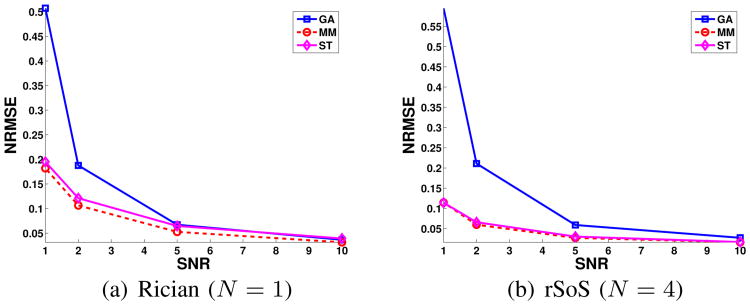
Noisy Rician magnitude images (N = 1) and NCC rSoS images (N = 4) were synthesized at several different SNRs (SNR = 1, 2, 5, and 10, with SNR defined as the ratio between the median value of the noiseless single-channel image magnitude and σ). TV denoising was performed using the MM, GA, and ST approaches described above, using perfect knowledge of the true value of σ². Five different noise realizations were generated at each SNR. For each method and each SNR, the TV regularization parameter λ was optimized to yield the smallest possible error with respect to the gold-standard noiseless image. Error was measured using the normalized root mean-squared error (NRMSE) metric, defined as $\mathrm{NRMSE}={\Vert \widehat{\mathbf{x}}-{\mathbf{x}}_{\mathrm{gold}}\Vert }_2/{\Vert {\mathbf{x}}_{\mathrm{gold}}\Vert }_2$, where $\widehat{\mathbf{x}}$ and x_gold are the estimated and gold-standard images, respectively. NRMSE was also used to quantify the performance of the different denoising methods. Since NRMSE has certain limitations [57], we also performed qualitative visual comparisons.

Quantitative results from these simulations are shown in Fig. 1, while qualitative visual results are shown in Figs. 2 and 3 and Supplementary Figs. S1 and S2⁵ (Figs. 2 and 3 show the Rician case, while Supplementary Figs. S1 and S2 show the rSoS case with N = 4). These results show that for all SNRs, the MM and ST images have substantially less error and bias than the GA images. This is not surprising because GA is based on an inaccurate noise model that completely neglects the noise bias, while MM and ST both incorporate information about the noise bias. Comparing MM and ST, both methods are effective at removing noise bias, though the MM results have smaller NRMSE values. This is also not surprising, since MM optimally models the full noise distribution, while the ST approach only models the bias.

Fig. 1.

Quantitative results for the TV denoising simulations. Each plot shows the NRMSE of each denoising method as a function of SNR.

Fig. 2.

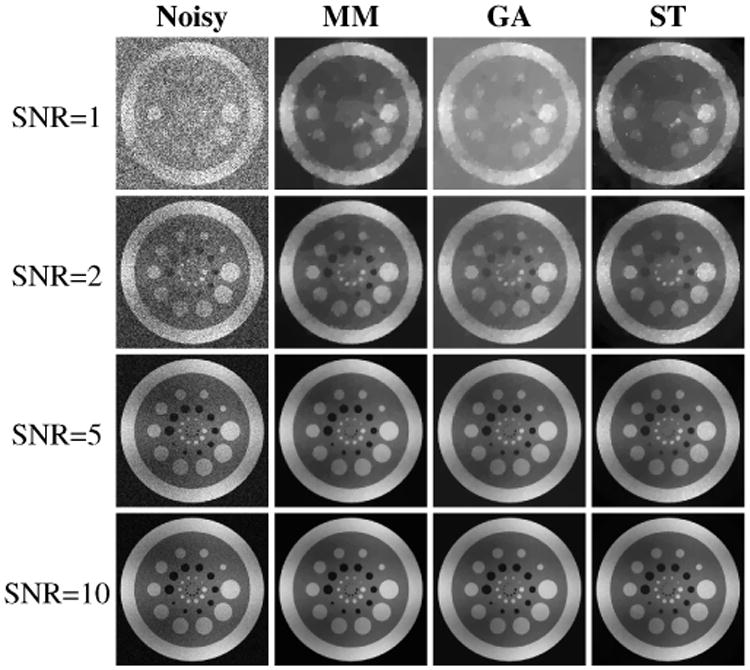
Representative results from TV denoising of simulated Rician data.

Fig. 3.

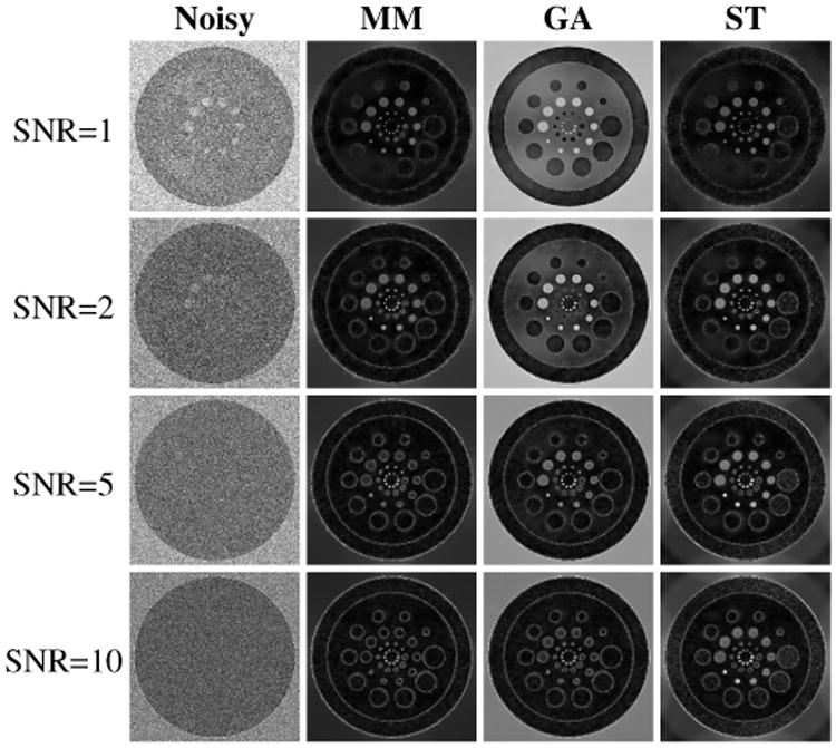
Root-mean-squared error images (computed based on five noise realizations) for the Rician TV denoising results shown in Fig. 2. For easier visualization, the image intensities for SNRs 1, 2, 5, and 10 were respectively scaled by factors of 1.5, 3, 6, and 10 relative to the images in Fig. 2.

While the NRMSE differences between MM and ST are relatively small in this simulation, the denoised images generated by these two approaches have an important qualitative difference. Specifically, we observe from Fig. 2 and Supplementary Fig. S1 that the ST approach smooths low-intensity image regions more strongly than high-intensity regions (i.e., image features in low-intensity regions look more blurred, while high-intensity image regions still have a speckled noisy appearance), while the MM approach appears to smooth all regions of the image in a scale-invariant manner. This behavior is especially evident at low SNRs, as highlighted in Supplementary Fig. S3 (which shows zoomed regions from Fig. 2). The uniform smoothing achieved by the MM approach should be expected, since TV is theoretically a scale-invariant regularization function [58]. On the other hand, applying TV leads to scale-variant behavior in the ST approach because the squaring and square-rooting operations used in ST are not scale-invariant.

B. Real Data

The proposed approach was also evaluated with real Rician and rSoS brain data. A high-resolution MPRAGE image (0.5×0.5×0.8 mm³ voxels with a matrix size of 384×384×192) was acquired with a 3T scanner and a 32-channel head coil. Fully-sampled raw k-space data was obtained for five different repetitions of the acquisition, and images were reconstructed using the standard Fourier transform. Denoising experiments were performed on a single-coil magnitude image and an rSoS image generated from the first repetition, while all five datasets were complex averaged to generate a “noiseless” gold standard reference images. We applied the unregularized ST approach to reduce any noise bias remaining in the gold standard images.

The proposed approach requires prior knowledge of σ² and N. We performed ML estimation of σ² based on data from background regions of the noisy images. Due to noise correlations between the different receiver coil elements in an rSoS image, the parameter N of the NCC distribution should not be chosen as the number of coils unless the receiver channels are prewhitened [18], [38]. As a result, we also performed ML estimation of N for the rSoS data, yielding an estimated value of N = 9. As shown in Supplementary Fig. S4, our estimated noise models match the empirical noise distributions quite accurately.

As in the simulations, TV denoising was performed using the MM, GA, and ST approaches, with regularization parameters for each method chosen to achieve a minimum NRMSE. Quantitative and qualitative results for Rician denoising are shown in Figs. 4 and 5, while rSoS results are shown in Supplementary Figs. S5 and S6. Consistent with the simulation results, both MM and ST substantially outperform the GA approach. In addition, MM yields smaller NRMSE and more uniform spatial smoothing than ST.

Fig. 4.

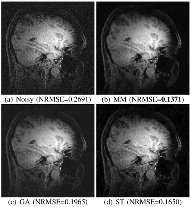
Results from Rician TV denoising of real brain data. Also shown are the NRMSE values for each image.

Fig. 5.

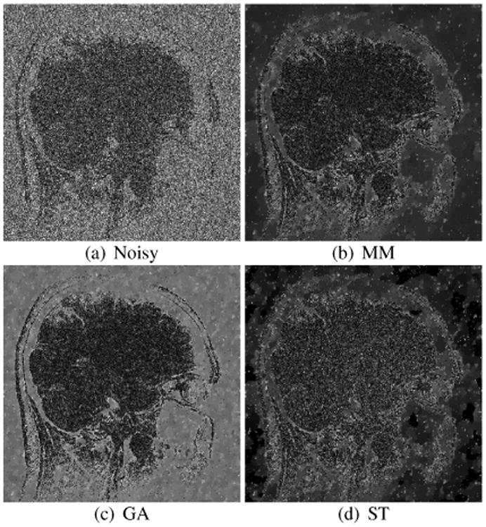
Error images for the Rician TV denoising results shown in Fig. 4. For easier visualization, the error image intensities were scaled by a factor of 4 relative to the images in Fig. 4.

V. Example Application: HARDI Estimation

Our second example involves the estimation of diffusion profiles from HARDI data [59], [60]. Briefly,⁶ HARDI acquisitions sample the diffusion-weighted MR signal on the surface of a sphere, with one set of spherical samples available for each imaging voxel. It is common to fit a spherical harmonic representation to this data to yield a continuous representation of the diffusion profile for each voxel [62]– [64]. The spherical harmonic basis for signals defined on the sphere is analogous to the Fourier series basis for periodic functions, and provides a convenient orthonormal basis that is widely used in a variety of applications. In HARDI, the fitted spherical harmonic representation can then be used to estimate the orientations of fiber structures within each voxel (useful for tracking white matter or muscle fibers through a process called tractography), and to estimate quantitative diffusion characteristics for each voxel like mean diffusivity (MD) and generalized fractional anisotropy (GFA). Parameters like MD and GFA provide insight into tissue microstructure and biomarkers for disease [60].

The use of magnitude images is especially prevalent in diffusion MRI, due to the fact that image phase is highly sensitive to subject motion in the presence of diffusion encoding. This leads to phase inconsistencies for in vivo data. In addition, the physics of the diffusion encoding process also means that diffusion MR images typically have low-SNR [17], [19], [20], [24], [25]. This combination of characteristics means that PML-based NCC modeling should be particularly attractive. However, most current HARDI studies denoise the data prior to estimation [17], [19], [20], and PML estimation has only been investigated to a limited extent [24]. Ref. [24] concluded that the PML approach is generally too computationally expensive to be worthwhile relative to simpler non-ML debiasing approaches. In this section, we demonstrate the potential value offered by our MM framework to enable computationally efficient PML HARDI estimation. It should be noted that [24] solved a maximum entropy spherical deconvolution problem for HARDI data, which is related but not identical to the more-common formulation based on Laplace-Beltrami regularized spherical harmonic estimation problem described below. To the best of our knowledge, this paper is the first work to evaluate PML methods for this formulation of the problem.

Given a data vector y of diffusion profile samples from a single voxel, commonly-used fitting procedures [61]–[64] estimate the spherical harmonic representation by solving

$$\widehat{\mathbf{x}}=arg\underset{\mathbf{x}}{min}\frac{1}{2{\sigma }^2}{\Vert \mathbf{A}\mathbf{x}-\mathbf{y}\Vert }_2^2+\lambda {\Vert \mathbf{L}\mathbf{x}\Vert }_2^2,$$ (14)

where the columns of the matrix A correspond to sampled versions of the truncated spherical harmonic basis functions,⁷ x is the unknown vector of spherical harmonic coefficients, λ is a regulation parameter, and L is either the identity matrix (to penalize signals with large ℓ₂-norm [63]) or the Laplace-Beltrami operator (to penalize non-smooth signals [64]).

Comparing with (1), Eq. (14) can be viewed as a GA-based form of spherical harmonic estimation. This GA estimator is easily computed using the noniterative linear LS solution [64]

$$\widehat{\mathbf{x}}={({\mathbf{A}}^H\mathbf{A}+2\lambda {\sigma }^2{\mathbf{L}}^H\mathbf{L})}^{-1}{\mathbf{A}}^H\mathbf{y}\triangleq \mathrm{\Phi }\mathbf{y}.$$ (15)

Instead of GA estimation, we investigate the use of NCC PML estimation as enabled by our proposed MM framework, by iterating according to:

$${\widehat{\mathbf{x}}}_{i+1}=arg\underset{\mathrm{x}:\mathbf{A}\mathrm{x}\ge 0}{min}\frac{1}{2{\sigma }^2}{\Vert \mathbf{A}\mathbf{x}-{\stackrel{\sim }{\mathbf{y}}}_i\Vert }_2^2+\lambda {\Vert \mathbf{L}\mathbf{x}\Vert }_2^2.$$ (16)

Equation. (16) has the simple solution ${\widehat{\mathbf{x}}}_{i+1}=\mathrm{\Phi }{\stackrel{\sim }{\mathbf{y}}}_{\mathit{i}}$ when $\mathbf{A}\mathrm{\Phi }{\stackrel{\sim }{\mathbf{y}}}_{\mathit{i}}$ is non-negative. When non-negativity is violated, we solve (16) as a standard quadratic programming problem using Matlab's quadprog function. The results we show later in this section are initialized by setting ${\widehat{\mathbf{x}}}_0$ equal to the non-negativity constrained solution to (14).

Our proposed MM approach was compared against the GA and ST approaches. For this problem, the ST approach debiases each measurement sample independently by subtracting the noise bias from magnitude-squared samples as described in the previous section, and then applies the standard GA estimator to the “debiased” data.

Laplace-Beltrami regularization was used in all cases, and the regularization parameter λ was individually optimized for each case to yield the smallest NRMSE.

A. Simulations

Noiseless diffusion data was simulated at M = 200 different points on the sphere, based on a two-tensor model given by

$$S({\mathbf{q}}_m)=\frac{S_0}{2}[e^{-b{\mathbf{q}}_m^H{\mathbf{D}}_1{\mathbf{q}}_m}+e^{-b{\mathbf{q}}_m^H{\mathbf{D}}_2{\mathbf{q}}_m}],$$ (17)

for m = 1, 2, …, M, where S(q_m) is the mth noiseless sample, S₀ is the signal without diffusion weighting, the diffusion encoding value is b =2,000 s/mm², the q_m are length-3 unit vectors describing the spherical sampling locations, and D₁ and D₂ are diffusion tensors [65] with identical eigenvalues (λ₁ = 1.4 × 10⁻³ mm²/s, λ₂ = λ₃ = 0.2 × 10⁻³ mm²/s) but different orientations. The angle between the principal eigenvectors of the two tensors was systematically varied from 0° to 90°. Complex Gaussian noise was added to the diffusion signal, and Rician data was obtained by taking the magnitude. Noisy data was simulated at SNR=3, 6, and 10, with SNR defined as S₀/σ. Estimation was performed 1000 times (using different noise realizations) for each case.

Estimation results were evaluated qualitatively and quantitatively. Quantitative performance was assessed using:

• Spherical Harmonic Error. Computed as the NRMSE of the estimated spherical harmonic coefficients with respect to those estimated from noiseless data.

• Mean Diffusivity (MD). Quantitative MD was computed according to [62]

  $$\mathit{\text{MD}}=-\frac{1}{bM}\sum _{m=1}^{M}ln({[\mathbf{A}\widehat{\mathbf{x}}]}_m/S_0+\epsilon ).$$ (18)

  where ε is a small regularization parameter used to reduce the sensitivity of the logarithm to small perturbations when ${[\mathbf{A}\widehat{\mathbf{x}}]}_{\mathit{m}}$ is near 0. This parameter was adjusted independently for each algorithm to yield minimal NRMSE.

• Generalized Fractional Anisotropy (GFA). The quantitative GFA diffusion measure was computed as [66]

  $$\sqrt{1-{[\widehat{\mathbf{c}}]}_1/{\Vert \widehat{\mathbf{c}}\Vert }_2^2]},$$ (19)

  where $\widehat{\mathbf{c}}$ is the spherical harmonic representation of the Funk-Radon Transform of $\widehat{\mathbf{x}}$ [60], and the first spherical harmonic coefficient [c]₁ corresponds to the isotropic spherical harmonic basis function.

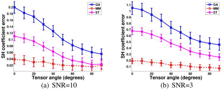
Quantitative simulation results are shown in Fig. 6 and Supplementary Fig. S7. Consistent with our previous results, Fig. 6 shows that the proposed MM method has the smallest spherical harmonic error at all SNRs, while Supplementary Fig. S7 shows that the MM method frequently yields MD and GFA estimates with the smallest bias. However, it should also be noted that MM can yield MD and GFA estimates with higher variance than GA or ST. This behavior (lower bias but higher variance) is consistent with previous studies involving the Rician distribution and the diffusion tensor model [25].

Fig. 6.

Quantitative spherical harmonic (SH) errors for the HARDI simulations. The lines and error bars respectively correspond to the means and standard deviations of the NRMSE values across 1000 noise realizations.

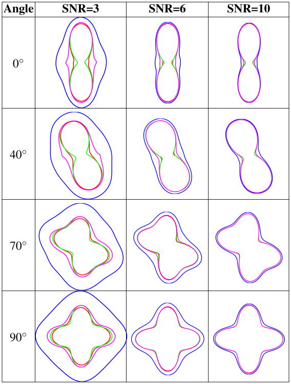
Qualitative results are shown in Fig. 7. We observe that all the methods work well at high SNR. As before, this is not surprising, since the Gaussian approximation is accurate at high SNR, while accurate noise modeling becomes more important at low SNR. At lower SNRs, both MM and ST yield substantially less bias than GA, while MM has slightly less bias than ST. These results further validate the potential benefits of using PML estimation with the MM framework.

Fig. 7.

Diffusion profile 2D cross-sections (passing through the plane defined by the principal eigenvectors of D₁ and D₂) computed from simulated data. Each image shows the noiseless profile (green) and average profiles estimated from noisy data using the MM (red), ST (magenta), and GA (blue) approaches.

B. Real Data

We also applied the MM approach to the 32-channel multi-shell diffusion imaging data from [17], with shells at b-values of 1,000, 2,000, 3,000, and 4,000 s/mm² and M = 30 samples per shell. Unlike [17] (which performed specialized k-space based denoising of the data), we used standard Fourier reconstruction of the data, with the complex images from each coil combined using rSoS.

Diffusion profiles from each shell were estimated separately within the HARDI framework using the MM, GA, and ST approaches. Noise parameters N and σ² were estimated as in Sec. IV-B. Since no gold standard is available, results were assessed qualitatively.

Results are shown in Fig. 8. It can be seen that both MM and ST are able to substantially reduce noise bias relative to GA. However, we also observe that the high b-value ST images possess much fewer low-intensity image structures relative to the MM and GA approaches, suggesting that it is less effective than MM at accurately preserving the diffusion profile. These results indicate that noise modeling during spherical harmonic estimation has potential benefits, and can complement the traditional approach where diffusion images are denoised prior to spherical harmonic estimation [17], [19], [20].

Fig. 8.

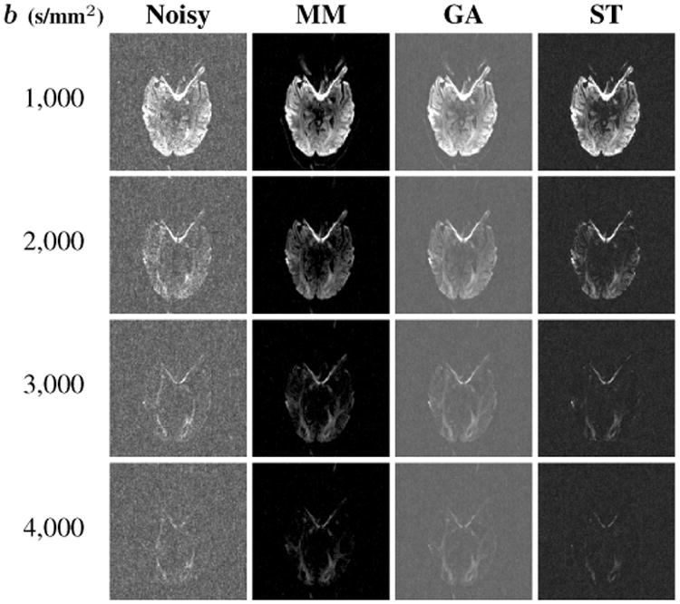
Representative real-data spherical harmonic estimation results. Each image row shows the estimated value of ${[\mathbf{A}\widehat{\mathbf{x}}]}_{\mathit{m}}$ for different choices of m corresponding to different b-values.

C. Comparisons with Traditional Optimization Algorithms

Our previous results focused on the benefits of using PML estimation instead of widely-used simplifed noise models. In this section, we compare the computational efficiency of our proposed MM approach against generic optimization algorithms that have been previously applied to solve NCC optimization problems. Specifically, we compared against standard quasi-Newton and Levenberg-Marquardt methods [44]. These algorithms were implemented using Matlab's fminunc and lsqnonlin functions, respectively, while our MM approach was evaluated using our own (relatively unoptimized) Matlab implementation. All algorithms were implemented with the same stopping criterion (iterations halted when the estimated change in spherical harmonic coefficients was less than 10⁻⁶, leading to a different number of iterations for each voxel and each algorithm. The number of MM iterations was limited to at most 100). Computations were performed using the same NCC-based cost function and 32-channel data from Sec. V-B, using a workstation with a quad-core 2.27 GHz processor. Spherical harmonic coefficients were estimated for all voxels within the FOV, and compute times were saved for each algorithm. The results obtained using MM had the smallest overall cost function values, ensuring that our compute times are not biased in favor of the MM approach.

Table I shows the mean and median compute times for each voxel, as well as the standard deviation and the total compute time for the whole image. The MM-based algorithm was much faster than the other PML algorithms for this data. In particular, the proposed MM algorithm was more than 16 × faster than the Levenberg-Marquardt method and more than 100× faster than the quasi-Newton method. Figure 9 compares the trade-off between compute time and statistical optimality between the PML and regularized non-ML methods. While the MM approach is not as fast as the non-ML GA and ST methods (with most compute times less than 4 ms per voxel), it yielded substantially smaller PML cost function values, providing a balance between quality and speed.

Table I.

Mean, median, standard deviation, and total compute times (units of seconds) for different PML algorithms.

Algorithm	Mean	Median	Stand. Dev.	Total
Quasi-Newton	1.923	2.010	0.516	31503.3
Levenberg-Marquardt	0.119	0.118	0.010	1941.3
MM	0.017	0.022	0.008	283.7

Fig. 9.

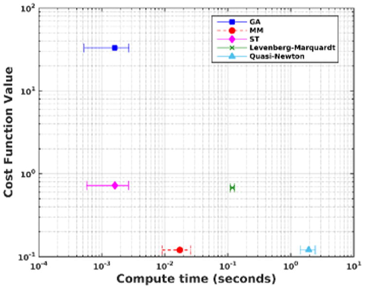
Plot of the cumulative PML cost function value for all voxels (normalized for easier visualization) versus the mean per-voxel compute time for different algorithms. The error bars show ± one standard deviation.

When interpreting these speed results, it should be noted that the computational efficiency of MM was dependent on the existence of efficient algorithms for solving regularized LS problems. For other cost functions where efficient regularized LS algorithms are not available, the MM approach may not be preferred. As with all optimization algorithms, computational efficiency is best examined individually for each context.

VI. Discussion

A. Initialization and Local Minima

Our empirical results indicate that the MM approach demonstrates better performance than the ST and GA methods for the applications we investigated. However, it is important to point out that the computational complexity of ST or GA is similar to the complexity of just one iteration of the MM approach, and that the MM approach needs to be initialized well for the difference in computation time to be negligible. Good initializations are also important because our work showed that the NCC NLL is generally nonconvex, and therefore subject to local minima. We are also aware of one specific initialization that is particularly problematic: if ${\widehat{\mathbf{x}}}_0$ is chosen such that $\mathcal{K}({\widehat{\mathbf{x}}}_0)=0$, then the corresponding ${\stackrel{\sim }{\mathbf{y}}}_0=0$, meaning that ${\widehat{\mathbf{x}}}_1$ will not depend in any way on the measured data y and that the MM framework can stagnate unless the regularization term R(x) specifically prefers nonzero solutions.

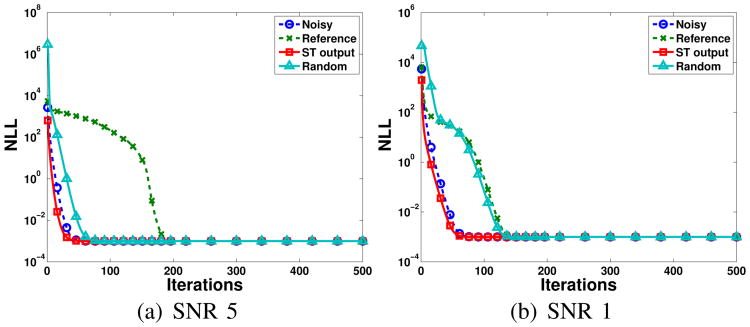
To empirically investigate convergence characteristics, we performed MM-based NCC image denoising as in Sec. IV-A for four different initializations: (i) initialization with the noisy image ${\widehat{\mathbf{x}}}_0=\mathbf{y}$, (ii) initialization with the true noiseless image, (iii) initialization with the unregularized ${\widehat{\mathbf{x}}}_{\mathrm{ST}}$ result, and (iv) random initialization. For each initialization, we ran 500 MM iterations while tracking the cost function value.

Figure 10 shows the results. It can be seen that the results of all the initializations converge to a similar cost function value, though different initializations converge faster than others. The resulting denoised images (not shown) are quite similar to one another, though do contain small differences in regions of the image where the true noiseless signal is zero. Even though the final results obtained from these different initializations only have minor differences for this denoising example, it is important to remember that there are initializations for which the MM approach will fail to come close to a useful solution (e.g., the all-zero initialization), and that other application contexts might be more severely impacted by nonconvexity. At least for this application, either the ST output or the noisy image seem like useful initializations for the MM approach, since both of these choices lead to fast convergence in Fig. 10.

Fig. 10.

Convergence plots for the MM approach with different initializations.

B. Accurate Noise Modeling

Using the NCC NLL from (7) relies on the prior knowledge of N and σ², and assumes that noise is white and uncorrelated from voxel to voxel and from coil to coil. However, there are practical situations where these assumptions might be violated. For example, it is frequently inaccurate to assume that the noise between different coils is uncorrelated and has the same variance. Previous work has shown that in such cases, rSoS data is still modeled accurately by an NCC distribution, except that the parameter N might not equal the number of images that were combined using rSoS [38], [67]–[70]. For this case, it has been shown that ML estimation of N yields reasonable results [38], and for simplicity, we used this approach in the results we presented. Alternatively, another common approach would be to prewhiten the data from different coils using the noise correlation matrix [2], and apply rSoS to these instead.

Since we used fully-sampled data and traditional Fourier reconstruction, our assumptions (that N and σ² were spatially invariant, and that noise in different voxels was uncorrelated) will be valid for all the results shown in this paper. This means that our noise modeling assumptions are expected to be accurate, as confirmed by Supplementary Fig. S3. However, depending on the provenance of the images, there are cases where the noise may be spatially correlated and/or spatially varying. For example, spatial noise correlations and spatially-varying noise parameters can exist if images are reconstructed using parallel imaging methods like GRAPPA [71] or SENSE [2]. Spatially-varying σ² values can also exist if images from multiple coils are combined using adaptive combination methods [72]. Fortunately, it has been observed that even if spatial noise correlation is neglected, there is still a benefit to modeling the data as if it were spatially-independent NCC [38]. In addition, there exist several schemes for directly estimating the parameters of spatially-varying noise fields from MRI images [38], [67]–[70], and there also exist methods for theoretically predicting noise parameters based on reconstruction parameters [73]. If spatially-varying noise parameters are known, the MM approach can be easily adapted: this would be achieved by replacing σ² and N in (7) by appropriate spatially-varying values that depend on m.

To illustrate this, we used the same 32-channel MPRAGE dataset from Sec. IV-B to generate GRAPPA-reconstructed images (acceleration factor 3) from single-repetition data. Images from each coil were combined using both rSoS and adaptive coil combination [72]. The combined images were subsequently denoised using TV regularization and the MM, GA, and ST methods. For each method, the cost function was modified on a voxel-by-voxel basis to account for spatially varying noise. We used the pseudo multiple replica method to generate synthetic noise with the same statistics as the real noise [73], and estimated spatially-varying σ² and N values using ML (with N = 1 for adaptively-combined data, since adaptively-combined images have Rician statistics). As before, the regularization parameter was tuned to yield minimum NRMSE for each method, with NRMSE calculated based on a fully-sampled 5×-averaged reference (debiased using ST).

Figs. 11 and 12 show the results for adaptively combined data, while Supplementary Figs. S8 and S9 show the rSoS results. As expected, the MM approach can successfully accommodate spatially-varying noise, and has better denoising performance than either GA or ST.

Fig. 11.

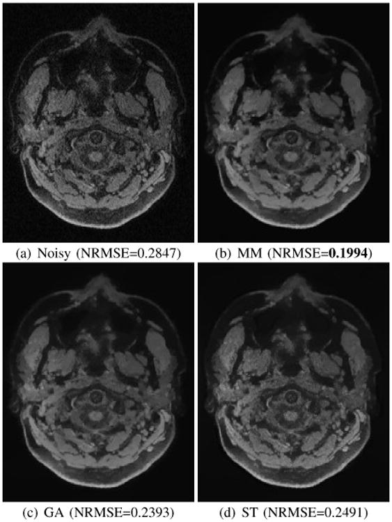
Results from GRAPPA reconstructed and adaptive combined TV denoising of real brain data. NRMSE values for each image are also shown.

Fig. 12.

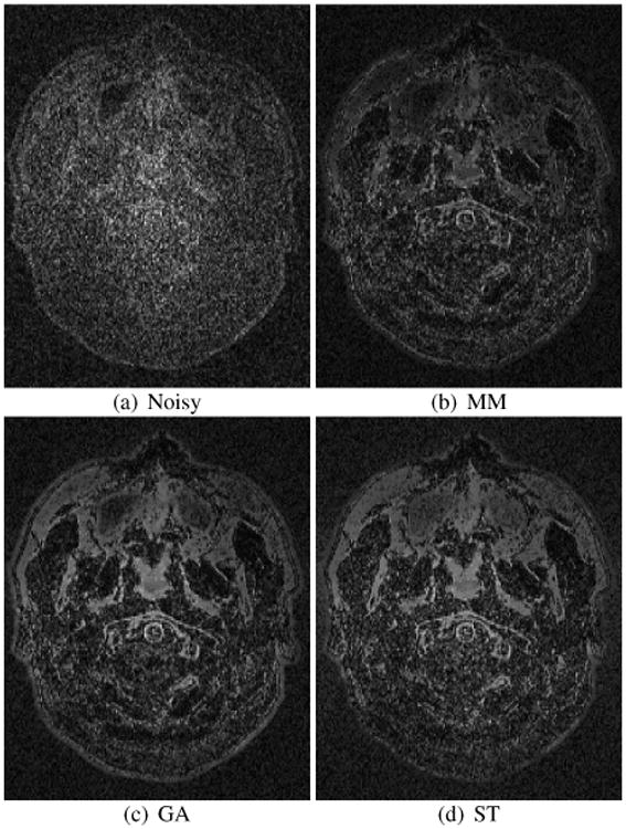
Error images for GRAPPA reconstructed and adaptive combined TV denoising results shown in Fig. 11. For easier visualization, the error image intensities were scaled by a factor of 4.2 relative to the images in Fig. 11.

In many data processing pipelines, it is common to also perform multiple preprocessing steps that could influence the noise distribution in the images. For example, motion correction, distortion correction, and bias field correction will all modify the characteristics of the noise distribution of an MR image in potentially undesirable ways that could invalidate the NCC assumptions. There are several possible ways of addressing this issue. A simple option would be to apply the NCC modeling at the first stage of the data processing pipeline. This is the approach we used in this paper (none of our data was preprocessed). Another option would be to keep track of the effects of each preprocessing stage on the overall noise distribution. For example, bias field correction will lead to a simple spatially-varying modification of σ² that can easily be computed if the bias field correction parameters are known. A final option might be to implement all of the different traditional image processing operations into a single integrated step. This might also have other advantages, since there is empirical evidence that supports the idea that integrated approaches yield better performance than stagewise processing in a variety of contexts (e.g., [74]–[76]).

It should also be noted that certain types of image reconstruction (e.g., nonlinear image reconstruction from sparsely-sampled and/or noisy data [3], [20]) could result in images with highly non-NCC statistical distributions. The proposed approach should be used with caution in such cases.

Consistent with previous reports [25], we observed that estimation using an accurate NCC model can decrease estimator bias, but can sometimes also increase variance. For applications where consistency is more important than systematic bias, approaches like GA might have certain advantages relative to accurate NCC modeling, and it is important to keep these trade-offs in mind when choosing a noise model for a specific MR application.

C. Choosing Images: Complex, Magnitude, or rSoS?

In principle, there are scenarios (e.g., when the original k-space data is available from each of multiple different receiver coils) in which investigators can choose whether to process multiple different Gaussian complex images, multiple different Rician magnitude images, or a single NCC-distributed rSoS image. It is natural to ask: which one of these options should be preferred? It is known from the data processing inequality [77] that we should theoretically expect for complex images to contain more information than magnitude images, and that magnitude images should contain more information than rSoS images, based on the fact that rSoS images can be computed from magnitude images, which themselves can be computed from complex images. Empirical confirmation of the advantage of complex images relative to Rician images for image denoising was shown in [17] and some of its references. However, Sijbers et al. [78] showed the surprising result that Gaussian complex images should only be preferred over Rician images in cases where the phase is relatively consistent, while estimation based on Rician distributed images can yield smaller RMSE when the phase is less predictable.

To the best of our knowledge, the question of whether to prefer complex images versus Rician images versus NCC images has never been addressed before. For this work, we performed a small-scale simulation study to provide insight. Specifically, we simulated a 4-coil data acquisition, where the noiseless image for each coil had constant phase and the same magnitude as the image used in Sec. IV-A, and each coil was subject to i.i.d. complex Gaussian noise. We compared the following schemes: (i) each complex image was denoised idependently using Gaussian modeling with TV regularization, followed by rSoS coil combination; (ii) the magnitude images from each coil were denoised independently using Rician modeling with TV regularization, followed by rSoS coil combination; (iii) the images were combined via rSoS, and then denoised using NCC modeling with TV regularization. Regularization parameters were independently optimized for each scheme and SNR to achieve minimal NRMSE.

Representative results are shown in Fig. 13. The results confirm the earlier finding that complex Gaussian images should be preferred when phase is consistent. However, it is interesting to note that NCC modeling outperforms Rician modeling. This can be partially attributed to the fact that rSoS coil combination has the effect of noise averaging, while the independent Rician denoising problems each have relatively lower SNR. Our evaluation in this subsection was intentionally brief, and different reconstruction and/or coil-combination strategies could easily lead to different conclusions (e.g., joint reconstruction [79] or adaptive coil combination [72]). In addition, images with different phase characteristics could yield very different results. For example, most MRI images have smooth phase, but spatial smoothing of complex images with rapidly varying phase would lead to poor results due to local phase cancellations. Despite the relatively small scope of the comparisons shown in Fig. 13, the main point we want to emphasize is that it's important to carefully consider how imaging data is stored and processed, since these decisions can have substantial impacts on the quality of the final results.

Fig. 13.

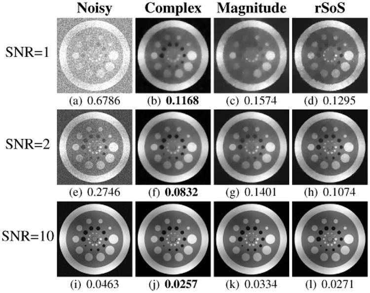
Comparison between TV denoising of complex, magnitude, and rSoS images. The NRMSE for each image is shown below each result.

VII. Conclusions

This paper proposed a new MM framework for statistical estimation problems involving NCC NLLs. Although we showed that NCC NLLs are generally nonconvex, the MM approach allows the optimization problem to be reduced into a series of simpler regularized LS problems. This enables the use of algorithms from the extensive body of literature on regularized LS optimization. Our empirical results validated that the use of the true NCC NLLs can have substantial performance advantages over commonly-used estimation approaches such as GA and ST that solve simplified optimization problems. In addition, we demonstrated that our proposed MM approach can have substantially lower compute time relative to traditional methods that are invoked for solving nonlinear optimization problems. The computational efficiency we observed is consistent with results reported by another group [80], who used our proposed MM framework (as we initially described in [46]) to achieve more than a 15× reduction in compute time for the denoising method described in [20].

Though we've only investigated the proposed framework in a couple scenarios, we expect it to be useful in a broad range of applications. A few examples include distortion correction for EPI images [34], non-negative matrix factorization [81], and compressed sensing diffusion MRI [5]–[9], among many others. The proposed framework is also a nice complement to recent tools for optimally choosing regularization parameters when dealing with NCC data [82].

References

- 1.Fessler JA. Model-based image reconstruction for MRI. IEEE Signal Process Mag. 2010;27:81–89. doi: 10.1109/MSP.2010.936726. [DOI] [PMC free article] [PubMed] [Google Scholar]
- 2.Pruessmann KP, Weiger M, Scheidegger MB, Boesiger P. SENSE: Sensitivity encoding for fast MRI. Magn Reson Med. 1999;42:952–962. [PubMed] [Google Scholar]
- 3.Lustig M, Donoho D, Pauly JM. Sparse MRI: The application of compressed sensing for rapid MR imaging. Magn Reson Med. 2007;58:1182–1195. doi: 10.1002/mrm.21391. [DOI] [PubMed] [Google Scholar]
- 4.Haldar JP. Low-rank modeling of local k-space neighborhoods (LORAKS) for constrained MRI. IEEE Trans Med Imag. 2014;33:668–681. doi: 10.1109/TMI.2013.2293974. [DOI] [PMC free article] [PubMed] [Google Scholar]
- 5.Michailovich O, Rathi Y, Dolui S. Spatially regularized compressed sensing for high angular resolution diffusion imaging. IEEE Trans Med Imag. 2011;30:1100–1115. doi: 10.1109/TMI.2011.2142189. [DOI] [PMC free article] [PubMed] [Google Scholar]
- 6.Landman BA, Bogovic JA, Wan H, El Shahaby FEZ, Bazin PL, Prince JL. Resolution of crossing fibers with constrained compressed sensing using diffusion tensor MRI. NeuroImage. 2012;59:2175–2186. doi: 10.1016/j.neuroimage.2011.10.011. [DOI] [PMC free article] [PubMed] [Google Scholar]
- 7.Bilgic B, Setsompop K, Cohen-Adad J, Yendiki A, Wald LL, Adelsteinsson E. Accelerated diffusion spectrum imaging with compressed sensing using adaptive dictionaries. Magn Reson Med. 2012;68:1747–1754. doi: 10.1002/mrm.24505. [DOI] [PMC free article] [PubMed] [Google Scholar]
- 8.Gramfort A, Poupon C, Descoteaux M. Denoising and fast diffusion imaging with physically constrained sparse dictionary learning. Med Image Anal. 2013;18:36–49. doi: 10.1016/j.media.2013.08.006. [DOI] [PubMed] [Google Scholar]
- 9.Paquette M, Merlet S, Gilbert G, Deriche R, Descoteaux M. Comparison of sampling strategies and sparsifying transforms to improve compressed sensing diffusion spectrum imaging. Magn Reson Med. 2015;73:410–416. doi: 10.1002/mrm.25093. [DOI] [PubMed] [Google Scholar]
- 10.Nowak RD. Wavelet-based Rician noise removal for magnetic resonance imaging. IEEE Trans Image Process. 1999;8:1408–1419. doi: 10.1109/83.791966. [DOI] [PubMed] [Google Scholar]
- 11.Sijbers J, den Dekker AJ, Van der Linden A, Verhoye M, Van Dyck D. Adaptive anisotropic noise filtering for magnitude MR data. Magn Reson Imag. 1999;17:1533–1539. doi: 10.1016/s0730-725x(99)00088-0. [DOI] [PubMed] [Google Scholar]
- 12.Pižurica A, Philips W, Lemahieu I, Acheroy M. A versatile wavelet domain noise filtration technique for medical imaging. IEEE Trans Med Imag. 2003;22:323–331. doi: 10.1109/TMI.2003.809588. [DOI] [PubMed] [Google Scholar]
- 13.He L, Greenshields IR. A nonlocal maximum likelihood estimation method for Rician noise reduction in MR images. IEEE Trans Med Imag. 2009;28:165–172. doi: 10.1109/TMI.2008.927338. [DOI] [PubMed] [Google Scholar]
- 14.Manjón JV, Coupé P, Martí-Bonmatí L, Collins DL, Robles M. Adaptive non-local means denoising of MR images with spatially varying noise levels. J Magn Reson Imag. 2010;31:192–203. doi: 10.1002/jmri.22003. [DOI] [PubMed] [Google Scholar]
- 15.Rajan J, Jeurissen B, Verhoye M, Audekerke JV, Sijbers J. Maximum likelihood estimation-based denoising of magnetic resonance images using restricted local neighborhoods. Phys Med Biol. 2011;56:5221. doi: 10.1088/0031-9155/56/16/009. [DOI] [PubMed] [Google Scholar]
- 16.Rajan J, Veraart J, Audekerke JV, Verhoye M, Sijbers J. Nonlocal maximum likelihood estimation method for denoising multiple-coil magnetic resonance images. Magn Reson Imag. 2012;30:1512–1518. doi: 10.1016/j.mri.2012.04.021. [DOI] [PubMed] [Google Scholar]
- 17.Haldar JP, Wedeen VJ, Nezamzadeh M, Dai G, Weiner MW, Schuff N, Liang ZP. Improved diffusion imaging through SNR-enhancing joint reconstruction. Magn Reson Med. 2013;69:277–289. doi: 10.1002/mrm.24229. [DOI] [PMC free article] [PubMed] [Google Scholar]
- 18.Aja-Fernández S, Brion V, Tristán-Vega A. Effective noise estimation and filtering from correlated multiple-coil MR data. Magn Reson Imag. 2013;31:272–285. doi: 10.1016/j.mri.2012.07.006. [DOI] [PubMed] [Google Scholar]
- 19.Brion V, Poupon C, Riff O, Aja-Fernández S, Tristán-Vega A, Mangin JF, LeBihan D, Poupon F. Noise correction for HARDI and HYDI data obtained with multi-channel coils and sum of squares reconstruction: An anisotropic extension of the LMMSE. Magn Reson Imag. 2013;31:1360–1371. doi: 10.1016/j.mri.2013.04.002. [DOI] [PubMed] [Google Scholar]
- 20.Lam F, Babacan SD, Haldar JP, Weiner MW, Schuff N, Liang ZP. Denoising diffusion-weighted magnitude MR images using rank and edge constraints. Magn Reson Med. 2014;71:1272–1284. doi: 10.1002/mrm.24728. [DOI] [PMC free article] [PubMed] [Google Scholar]
- 21.Leipert TK, Marquardt DW. Statistical analysis of NMR spin-lattice relaxation times. J Magn Reson. 1976;24:181–199. [Google Scholar]
- 22.Karlsen OT, Verhagen R, Bovée WMMJ. Parameter estimation from Rician-distributed data sets using a maximum likelihood estimator: application to T1 and perfusion measurements. Magn Reson Med. 1999;41:614–623. doi: 10.1002/(sici)1522-2594(199903)41:3<614::aid-mrm26>3.0.co;2-1. [DOI] [PubMed] [Google Scholar]
- 23.Sijbers J, den Dekker AJ, Raman E, Van Dyck D. Parameter estimation from magnitude MR images. Int J Imag Syst Tech. 1999;10:109–114. [Google Scholar]
- 24.Clarke RA, Scifo P, Rizzo G, Dell'Acqua F, Scotti G, Fazio F. Noise correction on Rician distributed data for fibre orientation estimators. IEEE Trans Med Imag. 2008;27:1242–1251. doi: 10.1109/TMI.2008.920615. [DOI] [PubMed] [Google Scholar]
- 25.Andersson JLR. Maximum a posteriori estimation of diffusion tensor parameters using a Rician noise model: Why, how and but. NeuroImage. 2008;42:1340–1356. doi: 10.1016/j.neuroimage.2008.05.053. [DOI] [PubMed] [Google Scholar]
- 26.Koay CG, Özarslan E, Basser PJ. A signal transformational framework for breaking the noise floor and its applications in MRI. J Magn Reson. 2009;197:108–119. doi: 10.1016/j.jmr.2008.11.015. [DOI] [PMC free article] [PubMed] [Google Scholar]
- 27.Noh J, Solo V. Rician distributed FMRI: Asymptotic power analysis and Cramér-Rao lower bounds. IEEE Trans Signal Process. 2011;59:1322–1328. [Google Scholar]
- 28.Kristoffersen A. Estimating non-Gaussian diffusion model parameters in the presence of physiological noise and Rician signal bias. J Magn Reson Imag. 2012;35:181–189. doi: 10.1002/jmri.22826. [DOI] [PubMed] [Google Scholar]
- 29.Bouhrara M, Reiter DA, Celik H, Bonny JM, Lukas V, Fishbein KW, Spencer RG. Incorporation of Rician noise in the analysis of biexponential transverse relaxation in cartilage using a multiple gradient echo sequence at 3 and 7 Tesla. Magn Reson Med. 2015;73:352–366. doi: 10.1002/mrm.25111. [DOI] [PMC free article] [PubMed] [Google Scholar]
- 30.Bai R, Koay CG, Hutchinson E, Basser PJ. A framework for accurate determination of the T2 distribution from multiple echo magnitude MRI images. J Magn Reson. 2014;244:53–63. doi: 10.1016/j.jmr.2014.04.016. [DOI] [PMC free article] [PubMed] [Google Scholar]
- 31.Sutton BP, Noll DC, Fessler JA. Fast, iterative image reconstruction for MRI in the presence of field inhomogeneities. IEEE Trans Med Imag. 2003;22:178–188. doi: 10.1109/tmi.2002.808360. [DOI] [PubMed] [Google Scholar]
- 32.Wilm BJ, Barmet C, Pavan M, Pruessmann KP. Higher order reconstruction for MRI in the presence of spatiotemporal field perturbations. Magn Reson Med. 2011;65:1690–1701. doi: 10.1002/mrm.22767. [DOI] [PubMed] [Google Scholar]
- 33.Hernando D, Karampinos DC, King JP, Haldar KF, Majumdar S, Georgiadis JG, Liang ZP. Removal of olefinic fat chemical shift artifact in diffusion MRI. Magn Reson Med. 2011;65:692–701. doi: 10.1002/mrm.22670. [DOI] [PMC free article] [PubMed] [Google Scholar]
- 34.Bhushan C, Joshi AA, Leahy RM, Haldar JP. Improved B0-distortion correction in diffusion MRI using interlaced q-space sampling and constrained reconstruction. Magn Reson Med. 2014;72:1218–1232. doi: 10.1002/mrm.25026. [DOI] [PMC free article] [PubMed] [Google Scholar]
- 35.Henkelman RM. Measurement of signal intensities in the presence of noise in MR images. Med Phys. 1985;12:232–233. doi: 10.1118/1.595711. [DOI] [PubMed] [Google Scholar]
- 36.McVeigh ER, Henkelman RM, Bronskill MJ. Noise and filtration in magnetic resonance imaging. Med Phys. 1985;12:586–591. doi: 10.1118/1.595679. [DOI] [PMC free article] [PubMed] [Google Scholar]
- 37.Dietrich O, Raya JG, Reeder SB, Ingrisch M, Reiser MF, Schoenberg SO. Influence of multichannel combination, parallel imaging and other reconstruction techniques on MRI noise characteristics. Magn Reson Imag. 2008;26:754–762. doi: 10.1016/j.mri.2008.02.001. [DOI] [PubMed] [Google Scholar]
- 38.Aja-Fernández S, Tristán-Vega A. A review on statistical noise models for magnetic resonance imaging. Universidad de Valladolid; 2013. Tech Rep LPI2013-01. [Google Scholar]
- 39.Constantinides CD, Atalar E, McVeigh ER. Signal-to-noise measurements in magnitude images from NMR phased arrays. Magn Reson Med. 1997;38:852–857. doi: 10.1002/mrm.1910380524. [DOI] [PMC free article] [PubMed] [Google Scholar]
- 40.Rice SO. Mathematical analysis of random noise. Bell Syst Technol J. 1944;23:282–332. [Google Scholar]
- 41.McGibney G, Smith MR. An unbiased signal-to-noise ratio measure for magnetic resonance images. Med Phys. 1993;20:1077–1078. doi: 10.1118/1.597004. [DOI] [PubMed] [Google Scholar]
- 42.Miller AJ, Joseph PM. The use of power images to perform quantitative analysis on low SNR MR images. Magn Reson Imag. 1993;11:1051–1056. doi: 10.1016/0730-725x(93)90225-3. [DOI] [PubMed] [Google Scholar]
- 43.Gudbjartsson H, Patz S. The Rician distribution of noisy MRI data. Magn Reson Med. 1995;34:910–914. doi: 10.1002/mrm.1910340618. [DOI] [PMC free article] [PubMed] [Google Scholar]
- 44.Bertsekas D. Nonlinear Programming. Athena Scientific. 1999 [Google Scholar]
- 45.Hunter DR, Lange K. A tutorial on MM algorithms. Am Stat. 2004;58:30–37. [Google Scholar]
- 46.Varadarajan D, Haldar JP. A quadratic majorize-minimize framework for statistical estimation with noisy Rician- and noncentral chi-distributed MR images. Proc IEEE Int Symp Biomed Imag. 2013:708–711. [Google Scholar]
- 47.Varadarajan D, Haldar JP. A novel approach for statistical estimation of HARDI diffusion parameters from Rician and non-central chi magnitude images. Proc Int Soc Magn Reson Med. 2014:801. [Google Scholar]
- 48.Solo V, Noh J. An EM algorithm for Rician fMRI activation detection. Proc IEEE Int Symp Biomed Imag. 2007:464–467. [Google Scholar]
- 49.Zhu H, Li Y, Ibrahim JG, Shi X, An H, Chen Y, Gao W, Lin W, Rowe DB, Peterson BS. Regression models for identifying noise sources in magnetic resonance images. J Amer Stat Assoc. 2009;104:623–637. doi: 10.1198/jasa.2009.0029. [DOI] [PMC free article] [PubMed] [Google Scholar]
- 50.Jacobsen MW, Fessler JA. An expanded theoretical treatment of iteration-dependent majorize-minimize algorithms. IEEE Trans Image Process. 2007;16:2411–2422. doi: 10.1109/tip.2007.904387. [DOI] [PMC free article] [PubMed] [Google Scholar]
- 51.Yuille AL, Rangarajan A. The concave-convex procedure. Neural Comput. 2003;15:915–936. doi: 10.1162/08997660360581958. [DOI] [PubMed] [Google Scholar]
- 52.Rudin LI, Osher S, Fatemi E. Nonlinear total variation based noise removal algorithms. Physica D. 1992;60:259–268. [Google Scholar]
- 53.Buades A, Coll B, Morel JM. Image denoising methods. a new nonlocal principle. SIAM Rev. 2010;52:113–147. [Google Scholar]
- 54.Venkatakrishnan SV, Bouman CA, Wohlberg B. Plug-and-play priors for model based reconstruction. Proc IEEE GlobalSIP. 2013:945–948. [Google Scholar]
- 55.Yang Z, Jacob M. Nonlocal regularization of inverse problems: A unified variational framework. IEEE Trans Image Process. 2013;22:3192–3203. doi: 10.1109/TIP.2012.2216278. [DOI] [PMC free article] [PubMed] [Google Scholar]
- 56.Chambolle A, Pock T. A first-order primal-dual algorithm for convex problems with applications to imaging. J Math Imaging Vis. 2011;40:120–145. [Google Scholar]
- 57.Wang Z, Bovik AC. Mean squared error: Love it or leave it? a new look at signal fidelity measures. IEEE Signal Process Mag. 2009;26:98–117. [Google Scholar]
- 58.Bouman C, Sauer K. A generalized Gaussian image model for edge-preserving MAP estimation. IEEE Trans Image Process. 1993;2:296–310. doi: 10.1109/83.236536. [DOI] [PubMed] [Google Scholar]
- 59.Tuch DS. PhD dissertation. Massachusetts Institute of Technology; 2002. Diffusion MRI of complex tissue structure. [Google Scholar]
- 60.Tuch DS. Q-ball imaging. Magn Reson Med. 2004;52:1358–1372. doi: 10.1002/mrm.20279. [DOI] [PubMed] [Google Scholar]
- 61.Haldar JP, Leahy RM. Linear transforms for Fourier data on the sphere: Application to high angular resolution diffusion MRI of the brain. NeuroImage. 2013;71:233–247. doi: 10.1016/j.neuroimage.2013.01.022. [DOI] [PMC free article] [PubMed] [Google Scholar]
- 62.Anderson AW. Measurement of fiber orientation distributions using high angular resolution diffusion imaging. Magn Reson Med. 2005;54:1194–1206. doi: 10.1002/mrm.20667. [DOI] [PubMed] [Google Scholar]
- 63.Hess CP, Mukherjee P, Han ET, Xu D, Vigneron DB. Q-ball reconstruction of multimodal fiber orientations using the spherical harmonic basis. Magn Reson Med. 2006;56:104–117. doi: 10.1002/mrm.20931. [DOI] [PubMed] [Google Scholar]
- 64.Descoteaux M, Angelino E, Fitzgibbons S, Deriche R. Regularized, fast, and robust analytical Q-ball imaging. Magn Reson Med. 2007;58:497–510. doi: 10.1002/mrm.21277. [DOI] [PubMed] [Google Scholar]
- 65.Basser PJ, Mattiello J, LeBihan D. Estimation of the effective self-diffusion tensor from the NMR spin echo. J Magn Reson B. 1994;103:247–254. doi: 10.1006/jmrb.1994.1037. [DOI] [PubMed] [Google Scholar]
- 66.Assemlal HE, Tschumperlé D, Brun L. Fiber tracking on HARDI data using robust ODF fields. Proc IEEE Int Conf Image Process. 2007:133–136. [Google Scholar]
- 67.Aja-Fernández S, Tristán-Vega A, Alberola-López C. Noise estimation in single-and multiple-coil magnetic resonance data based on statistical models. Magn Reson Imag. 2009;27:1397–1409. doi: 10.1016/j.mri.2009.05.025. [DOI] [PubMed] [Google Scholar]
- 68.Aja-Fernández S, Tristán-Vega A, Hoge WS. Statistical noise analysis in GRAPPA using a parametrized noncentral chi approximation model. Magn Reson Med. 2011;65:1195–1206. doi: 10.1002/mrm.22701. [DOI] [PMC free article] [PubMed] [Google Scholar]
- 69.Aja-Fernández S, Tristán-Vega A. Influence of noise correlation in multiple-coil statistical models with sum of squares reconstruction. Magn Reson Med. 2012;67:580–585. doi: 10.1002/mrm.23020. [DOI] [PubMed] [Google Scholar]
- 70.Brion V, Poupon C, Riff O, Aja-Fernandez S, Tristan-Vega A, Mangin JF, Le Bihan D, Poupon F. Parallel MRI noise correction: An extension of the LMMSE to non central chi distributions. Proc MICCAI. 2011:226–233. doi: 10.1007/978-3-642-23629-7_28. [DOI] [PubMed] [Google Scholar]
- 71.Griswold MA, Jakob PM, Heidemann RM, Nittka M, Jellus V, Wang J, Kiefer B, Haase A. Generalized autocalibrating partially parallel acquisitions (GRAPPA) Magn Reson Med. 2002;47:1202–1210. doi: 10.1002/mrm.10171. [DOI] [PubMed] [Google Scholar]
- 72.Walsh DO, Gmitro AF, Marcellin MW. Adaptive reconstruction of phased array MR imagery. Magn Reson Med. 2000;43:682–690. doi: 10.1002/(sici)1522-2594(200005)43:5<682::aid-mrm10>3.0.co;2-g. [DOI] [PubMed] [Google Scholar]
- 73.Robson PM, Grant AK, Madhuranthakam AJ, Lattanzi R, Sodickson DK, McKenzie CA. Comprehensive quantification of signal-to-noise ratio and g-factor for image-based and k-space-based parallel imaging reconstructions. Magn Reson Med. 2008;60:895–907. doi: 10.1002/mrm.21728. [DOI] [PMC free article] [PubMed] [Google Scholar]
- 74.Sutton BP, Noll DC, Fessler JA. Dynamic field map estimation using a spiral-in/spiral-out acquisition. Magn Reson Med. 2004;51:1194–1204. doi: 10.1002/mrm.20079. [DOI] [PubMed] [Google Scholar]
- 75.Ying L, Sheng J. Joint image reconstruction and sensitivity estimation in SENSE (JSENSE) Magn Reson Med. 2007;57:1196–1202. doi: 10.1002/mrm.21245. [DOI] [PubMed] [Google Scholar]
- 76.Tao S, Trzasko JD, Shu Y, Huston J, Bernstein MA. Integrated image reconstruction and gradient nonlinearity correction. Magn Reson Med. 2015 doi: 10.1002/mrm.25487. in Press. [DOI] [PMC free article] [PubMed] [Google Scholar]
- 77.Cover TM, Thomas JA. Elements of Information Theory. New York: John Wiley & Sons, Inc.; 1991. [Google Scholar]
- 78.Sijbers J, den Dekker AJ. Maximum likelihood estimation of signal amplitude and noise variance from MR data. Magn Reson Med. 2004;51:586–594. doi: 10.1002/mrm.10728. [DOI] [PubMed] [Google Scholar]
- 79.Haldar JP, Liang ZP. Joint reconstruction of noisy high-resolution MR image sequences. Proc IEEE Int Symp Biomed Imag. 2008:752–755. [Google Scholar]
- 80.Lam F, Liu D, Song Z, Weiner MW, Schuff N, Liang ZP. A fast algorithm for rank and edge constrained denoising of magnitude diffusion-weighted images. Proc Int Soc Magn Reson Med. 2014:401. doi: 10.1002/mrm.25643. [DOI] [PMC free article] [PubMed] [Google Scholar]
- 81.Sajda P, Du S, Brown TR, Stoyanova R, Shungu DC, Mao X, Parra LC. Nonnegative matrix factorization for rapid recovery of constituent spectra in magnetic resonance chemical shift imaging of the brain. IEEE Trans Med Imag. 2004;23:1453–1465. doi: 10.1109/TMI.2004.834626. [DOI] [PubMed] [Google Scholar]
- 82.Luisier F, Blu T, Wolfe PJ. A CURE for noisy magnetic resonance images: chi-square unbiased risk estimation. IEEE Trans Image Process. 2012;21:3454–3466. doi: 10.1109/TIP.2012.2191565. [DOI] [PubMed] [Google Scholar]
Associated Data
This section collects any data citations, data availability statements, or supplementary materials included in this article.