Fiber estimation and tractography in diffusion MRI: Development of simulated brain images and comparison of multi-fiber analysis methods at clinical b-values

Abstract

Advances in diffusion-weighted magnetic resonance imaging (DW-MRI) have led to many alternative diffusion sampling strategies and analysis methodologies. A common objective among methods is estimation of white matter fiber orientations within each voxel, as doing so permits in-vivo fiber-tracking and the ability to study brain connectivity and networks.

Knowledge of how DW-MRI sampling schemes affect fiber estimation accuracy, and consequently tractography and the ability to recover complex white-matter pathways, as well as differences between results due to choice of analysis method and which method(s) perform optimally for specific data sets, all remain important problems, especially as tractography-based studies become common.

In this work we begin to address these concerns by developing sets of simulated diffusion-weighted brain images which we then use to quantitatively evaluate the performance of six DW-MRI analysis methods in terms of estimated fiber orientation accuracy, false-positive (spurious) and false-negative (missing) fiber rates, and fiber-tracking. The analysis methods studied are: 1) a two-compartment “ball and stick” model (BSM) (Behrens et al., 2003); 2) a non-negativity constrained spherical deconvolution (CSD) approach (Tournier et al., 2007); 3) analytical q-ball imaging (QBI) (Descoteaux et al., 2007); 4) q-ball imaging with Funk-Radon and Cosine Transform (FRACT) (Haldar and Leahy, 2013); 5) q-ball imaging within constant solid angle (CSA) (Aganj et al., 2010); and 6) a generalized Fourier transform approach known as generalized q-sampling imaging (GQI) (Yeh et al., 2010). We investigate these methods using 20, 30, 40, 60, 90 and 120 evenly distributed q-space samples of a single shell, and focus on a signal-to-noise ratio (SNR = 18) and diffusion-weighting (b = 1000 s/mm²) common to clinical studies.

We found the BSM and CSD methods consistently yielded the least fiber orientation error and simultaneously greatest detection rate of fibers. Fiber detection rate was found to be the most distinguishing characteristic between the methods, and a significant factor for complete recovery of tractography through complex white-matter pathways. For example, while all methods recovered similar tractography of prominent white matter pathways of limited fiber crossing, CSD (which had the highest fiber detection rate, especially for voxels containing three fibers) recovered the greatest number of fibers and largest fraction of correct tractography for a complex three-fiber crossing region.

The synthetic data sets, ground-truth, and tools for quantitative evaluation are publically available on the NITRC website as the project “Simulated DW-MRI Brain Data Sets for Quantitative Evaluation of Estimated Fiber Orientations” at http://www.nitrc.org/projects/sim_dwi_brain

1. Introduction

Diffusion-weighted MRI (DW-MRI) (Beaulieu, 2002; LeBihan et al., 1986) is a unique imaging modality in which the diffusion of water molecules is used as a non-invasive probe of tissue microstructure. In this work we are particularly interested in the utility of DW-MRI to infer the orientation of coherently oriented bundles of axons in the brain's white-matter. By application of fiber-tracking algorithms (Mori and van Zijl, 2002) the orientation information can be used to generate so-called tractograms, which are depictions of estimated white-matter connections between populations of neurons in gray-matter (Conturo et al., 1999; Mori et al., 1999).

In recent years tractography has found extensive application. A not exhaustive list includes neuroanatomical studies and atlases (e.g. Catani and Thiebaut de Schotten, 2008), neurosurgical planning (e.g. Golby et al., 2011) and post-surgery evaluation, and many aspects of assessment and study of neurological diseases such as multiple sclerosis (e.g. Mesaros et al., 2012), Alzheimer's disease (e.g. Morikawa et al., 2010) and schizophrenia (e.g. Voineskos et al., 2010). Tractography has also been instrumental in neurobehavioral modeling, where, for example, it contributed to an improved model of the limbic system (Catani et al., 2013). More recently tractography has been used to identify auditory pathways between the auditory thalamus/brainstem and different areas of auditory analysis in the cortex (Javad et al., 2014). Such non-invasive assessment of white-matter morphology could improve the prognosis of recovery of useful hearing following cochlear implantation, as the latter is influenced by the integrity of subcortical pathways (Vlastarakos et al., 2010). Last, white-matter tractography permits in-vivo graph theoretical analysis of structural brain networks (Bullmore and Sporns, 2009), and as such fulfills a fundamental role in mapping the human connectome (Toga el al., 2012).

An important step towards further clinical application of tractography is a broader understanding of how the data acquisition, analysis method and fiber-tracking algorithm, each affect track reconstruction. Also, it is beneficial to know which analysis method yields the most complete and accurate tractography when applied to DW data acquired with a particular set of parameters. While tractography is strongly dependent on the fiber-tracking algorithm itself, results are fundamentally determined by the DW-MRI analysis methods’ ability to resolve crossing fibers and provide accurate estimates of their orientations. Development of appropriate synthetic DW-MRI data sets, with ground-truth and quantitative metrics for evaluating the fiber estimation performance of multi-fiber analysis methods, and an examination of how results impact tractography, is the focus of this paper.

Background

The most common approach to DW-MRI analysis is Diffusion Tensor Imaging (DTI) (Basser et al., 1994a, 1994b; Basser and Pierpaoli, 1996), which models the diffusion of water molecules by a single rank-2 tensor (a 3×3 symmetric matrix). The method is popular because considerable quantitative information, such as fractional anisotropy (FA), mean diffusivity (MD) and white-matter fiber orientation, can be obtained robustly from relatively small data sets (Jones, 2004). However, DTI is limited to modeling a single-fiber orientation per voxel and is therefore incapable of resolving complex intra-voxel geometry such as crossing-fibers (Alexander et al., 2002; Frank, 2001; Tuch et al., 2002), which are thought to occur in at least one-third of voxels in white-matter (Behrens et al., 2007). To overcome this problem, many alternative multi-fiber analysis methods have been proposed.

The alternatives include high-angular resolution diffusion imaging (HARDI) methods, such as a family of q-ball imaging (Canales-Rodríguez et al., 2009; Descoteaux et al., 2007; Hess et al., 2006; Michailovich and Rathi, 2010; Tuch, 2004) and many other variants of the methods listed here, and spherical deconvolution approaches (Dell'Acqua et al., 2010; Tournier et al., 2004, 2007), which sample single or multiple shells in q-space, and methods based on Cartesian sampling schemes of q-space, such as diffusion spectrum imaging (DSI) (Tuch et al., 2003; Wedeen et al., 2005, 2008), DSI with partial sampling schemes (Kuo et al., 2013; Yeh et al., 2008), and related variant (Canales-Rodríguez et al., 2010). This list is not exhaustive and a great many other model and non-model based methods exist; see (Assemlal et al., 2011; Haldar and Leahy, 2013) for a more comprehensive list and theoretical differences.

As multi-fiber analysis is a relatively young field, much of the initial work has focused on development of new methods, which are often presented with simulation studies for comparison against a few alternatives, however differences in signal models, simulation parameters and/or evaluation metrics usually prevent a broader comparison of similar work. Combined with variations in data sets (e.g. number and magnitude of diffusion-weighting directions, or SNR), often it remains unclear whether new methods are improvements over existing approaches, and if so, under what conditions.

Towards quantitative evaluation

Many diffusion phantoms have been developed for validation of DW-MRI analysis methods, such as biological phantoms constructed from rat spinal cord (Campbell et al., 2005), spherical (Moussavi-Biugui et al., 2010) or straight (Pullens et al., 2010) crossings of polyester fibers, and planar phantoms of various materials including water-filled plastic capillaries (Tournier et al., 2008), permeable Rayon fibers (Perrin et al., 2005), solid acrylic fibers (Poupon et al., 2008), or polyethylene fibers (Farrher et al., 2012), and many more. These phantoms have generally consisted of simple geometry (e.g. a single crossing-fiber region) for basic DW-MRI validation purposes, and as such have not been used for detailed characterization and comparison of analysis methods.

The “Fiber Cup” phantom (Fillard et al., 2011; Poupon et al., 2010) and contest (MICCAI 2009 conference, http://www.lnao.fr/spip.php?rubrique79) was purposely developed to address the lack of a publicly available diffusion-weighted data set including tractography ground-truth and evaluation tools to aid comparison of analysis methods. The Fiber Cup is a planar phantom with fiber configurations modeled from a coronal cross-section of the brain. Overall it consists of seven fiber branches having three fiber crossings, one merging/diverging region, and one fiber splitting region. As Fiber Cup data is publicly available it has been frequently used for both qualitative and quantitative evaluation of DW-MRI analysis methods and tractography. In addition, an online tool “Tractometer” (Côté et al., 2013; http://tractometer.org) is available for connectivity-based evaluation of reconstructed Fiber Cup tracks, permitting extensive comparison of data analysis methods and tractography algorithms.

Fiber Cup is geared towards tractography evaluation however, and as such is not suited to detailed characterization of fiber estimation performance – the phantom has few crossing angles, and without a ground-truth of orientations it is impossible to quantify the accuracy of estimated fibers. Furthermore, one cannot distinguish between estimated fibers that are representative of the ground-truth, or are artifacts of the analysis method. A more recent “HARDI reconstruction challenge” (ISBI 2012 conference, http://hardi.epfl.ch/static/events/2012_ISBI; Daducci et al., 2013) attends to these issues by use of simulated DW phantoms which offer considerable versatility (e.g. choice of signal model, diffusion sampling schemes, signal to noise ratio, and known fiber ground-truth) over physical phantoms, albeit over-simplifying the real diffusion process and MR signal. In comparison to Fiber Cup, the HARDI challenge focuses exclusively on intra-voxel multi-fiber estimation.

New DW-MRI data sets and quantitative tools

The contributions of this work are two-fold. First is the development of synthetic brain-like diffusion-weighted data sets based on a ground-truth of fiber orientations estimated from in-vivo data, in conjunction with quantitative measures associated with fiber detection accuracy (false-positives, false-negatives, and individual fiber orientation error) and tractography. Second is application of synthetic data resembling a typical clinical acquisition to compare six well-known DW-MRI analysis methods.

Developing the ground-truth from in-vivo data has the advantage of preserving realistic crossing-fiber configurations, and ability to observe the implications of fiber estimation accuracy on tractography, which is of crucial importance to brain network and human connectome studies (Bastiani et al., 2012; Cheng et al., 2012; Gigandet et al., 2013). Furthermore, both Fiber Cup and HARDI reconstruction challenge data sets contain large fiber tracks (at least 3 voxels in width) with adjacent slices having identical structure. This means each voxel is surrounded by a neighborhood of similar or identical voxels which is unrealistic of real white-matter configurations and could bias analysis methods that make use of neighborhood information. We avoid this problem and preserve realistic neighborhood information by deriving the ground-truth from in-vivo data.

While several aspects of our work are similar to those of the HARDI reconstruction challenge (Daducci et al., 2013), such as the choice of fiber estimation metrics, there are important differences between the simulation models and the overall goals. Specifically, we include a free diffusion compartment in the signal model to accommodate sources of isotropic diffusion, as well as T₂-weighting MR signal decay, which both impact fiber estimation accuracy, even in the simple case of single fiber estimation. Overall, our goal is to determine which analysis method is optimal for clinically acquired data, whereas in (Daducci et al., 2013) each method is evaluated with a custom (optimal) data set, meaning the outcomes reflect the best possible result for each analysis method.

A previous simulation study (Ramirez-Manzanares et al., 2011) evaluated several HARDI-based methods using model and non-model based techniques for synthesizing clinical-like DW-MRI data at different SNR, however the compartment sizes for individual fibers were fixed to few discrete values and did not accommodate free diffusion, fiber crossing angles were limited to ≥ 30° for voxels with 2 fibers and fixed to 90° for voxels with 3 fibers, and no T₂-weighting of the MR signal was present. By developing our simulation from in-vivo data we were able to avoid such constraints, leading to more comprehensive evaluation.

After generating the synthetic data we compare the following six multiple-fiber diffusion analysis methods: 1) a two-compartment “ball and stick” model (BSM) (Behrens et al., 2003); 2) a non-negativity constrained spherical deconvolution (CSD) approach (Tournier et al., 2007); 3) analytical q-ball imaging (QBI) (Descoteaux et al., 2007); 4) q-ball imaging with Funk-Radon and Cosine Transform (FRACT) (Haldar and Leahy, 2013); 5) q-ball imaging within constant solid angle (CSA) (Aganj et al., 2010); and 6) a generalized Fourier transform approach known as generalized q-sampling imaging (GQI) (Yeh et al., 2010). To investigate the effect of diffusion sampling each method is evaluated using 20, 30, 40, 60, 90 and 120 evenly distributed q-space samples of a single shell, at an SNR = 18 and diffusion-weighting (1000 s/mm²) common to clinical studies.

2. Material and Methods

In this section we establish the ground-truth, define the data synthesis model, and present the quantitative metrics for comparison of results.

2.1 Establishment of simulation ground-truth

A 28-year-old right-handed male volunteer without any history of neurological disease was scanned on a GE 3T HDxt scanner (General Electric, Milwaukee, WI, USA), equipped with an 8-channel head coil. The subject signed an informed consent form for which the imaging protocol was approved by the Institutional Review Board of the University of Southern California.

A DW data set was acquired by a twice-refocused pulsed-gradient spin-echo (PGSE) sequence with TE/TR = 83.4 ms/16100 ms, acquisition matrix = 128×128, ASSET acceleration factor of 2, voxel size = 2.4×2.4×2.4 mm, 60 contiguous slices, 150 diffusion gradient directions with diffusion-weighting b = 1000 s/mm², and 10 non-diffusion weighted volumes. The acquisition took approximately 43 minutes.

Without eddy-current or motion correction¹ the diffusion data set was processed by the probabilistic multi-fiber “ball and stick” method implemented in the program ‘bedpostx’, a part of the diffusion toolbox in the FMRIB Software Library (FSL v5.0.2.2; http://www.fmrib.ox.ac.uk/fsl; Behrens et al., 2003; Smith et al., 2004). Up to three fibers were estimated per voxel. To reduce the possibility of false minor fibers resulting from data over-fitting, a threshold of 0.1 was applied to second and third fiber volume fractions. Images of number of fibers/voxel were inspected to ensure known crossing regions (as explored later in Sect. 3.5) retained 2 or 3 fibers after thresholding.

Our synthetic DW data sets are derived from the fiber volume fractions (f₁,f₂,f₃) and orientations (v₁,v₂,v₃) estimated for each voxel and output by ‘bedpostx’. Because of differences between the “ball and stick” model and our data synthesis equation, Eq. (1), the isotropic compartment fraction (f₀) was not used. Instead, the fiber fractions were normalized (${\sum }_{k=1}^3{f}_k=1$) and f₀ was iteratively determined per voxel: beginning with f₀ = 0, f₀ was gradually increased until the generalized fractional anisotropy (GFA) (Tuch, 2004) of the synthetic data reduced to within 0.00005 of the GFA of the corresponding in-vivo data.

Anatomical T₁-weighted SPGR images (TE/TR = 2.856 ms/7 ms) were acquired with a voxel size of 1×1×1 mm. The anatomical volume was registered to the mean non-diffusion weighted volume and subsequently segmented into white-matter (WM), gray-matter (GM) and cerebrospinal fluid (CSF) using default options in SPM (SPM v8; http://www.fil.ion.ucl.ac.uk/spm; Friston et al., 1995). The high-resolution tissue probability maps were then down-sampled by linear interpolation to the resolution of the DW data, and each voxel was classified as WM, GM, or CSF according to its most probable tissue type.

2.2 Diffusion-weighted data synthesis

Diffusion-weighted data were synthesized according to a multi-tensor model (Alexander et al., 2001; Tuch et al., 2002) accommodating three crossing fibers per voxel in addition to a free-diffusion compartment. For any given voxel the signal model is:

$$S(b,{\mathit{g}}_j)=S_0[f_0\exp (-b{D}_0)+(1-f_0){\sum }_{k=1}^3{f}_k\exp (-b{\mathit{g}}_j^T{\mathit{D}}_k{\mathit{g}}_j)]$$ (1)

where S₀ simulates T₂-weighting, f₀ and D₀ are the volume fraction and diffusivity, respectively, of the isotropic free-diffusion compartment, f_k and D_k are the volume fraction and diffusion tensor, respectively, of the k^th fiber in the voxel, b is the diffusion-weighting, and g_j is a unit vector representing the j^th gradient direction. Altogether the volume fractions satisfy $f_0+(1-f_0){\sum }_{k=1}^3{f}_k=1$.

Each fiber's diffusion tensor, D_k , was computed by rotating a default single tensor, D_x . That is D_k = R_x(v_k)D_xR_x(v_k)^T , where v is a vector defining the desired fiber orientation, R_x(v) is the rotation matrix that aligns the vector x =[100]^T oriented along the x-axis to v , and D_x is the single-fiber tensor model with diffusivities in orthogonal directions given by λ_1,2,3. (Tuch, 2004)

$${\mathit{R}}_{\mathit{x}}\left(\mathit{v}\right)=\frac{(\mathit{x}+\mathit{v}){(\mathit{x}+\mathit{v})}^{\mathit{T}}}{({\mathit{x}}^{\mathit{T}}\mathit{v}+1)}-\mathit{I}$$ (2)

$${\mathit{D}}_{\mathit{x}}=\left[\begin{array}{ccc}\hfill {\lambda }_1\hfill & \hfill 0\hfill & \hfill 0\hfill \\ \hfill 0\hfill & \hfill {\lambda }_2\hfill & \hfill 0\hfill \\ \hfill 0\hfill & \hfill 0\hfill & \hfill {\lambda }_3\hfill \end{array}\right]$$ (3)

Complex Gaussian noise was added to the synthesized signal, S, to achieve a Rician distribution of noisy magnitude diffusion data (Gudbjartsson and Patz, 1995):

$$E(b,{\mathit{g}}_j)=\sqrt{{\left(S\left(b,{\mathit{g}}_j\right)+\frac{n_1}{\sqrt{2}}\right)}^2+{\left(\frac{n_2}{\sqrt{2}}\right)}^2}$$ (4)

where n₁ and n₂ are independent and identically distributed Gaussian random variables with zero mean and standard deviation σ_n = μ_s0/SNR , in which μ_s0 is the mean signal from a homogeneous white-matter region of the S₀ non-diffusion weighted image, and SNR is the desired signal-to-noise ratio of the magnitude image, E.

2.3 Quantitative metrics

Analyzed synthetic DW data sets were evaluated against the ground-truth in terms of fiber orientation error, rate of spurious fibers (false-positives), rate of missing true fibers (false-negatives), and fraction of similar (overlapping) and dissimilar (non-overlapping) voxelized tractography. The fiber orientation and false rate metrics are consistent with those used in similar work (Daducci et al., 2013).

2.3.1 Individual fiber orientation error

The fiber orientation error is the angular separation between pairs of estimated and actual fiber orientations, and lies in the range 0–90°. In this study, we report individual fiber orientation errors for the unique pairing of estimated and actual fiber orientations that yields the minimum total orientation error. Each estimated fiber orientation is paired with only one actual fiber orientation from the ground-truth.

2.3.2 False-positive and false-negative rate

The number of incorrect fibers (either false-positives or false-negatives) was computed as the signed difference between the number of estimated and actual fibers (from the ground-truth) on a voxel-by-voxel basis. In this way, +1 indicates a single spurious fiber, whereas -2 indicates two missing fibers. The total number of false-positives and false-negatives was computed separately and expressed as a percentage of the actual number of fibers present; positive false rates (> 0%) indicate false-positives (spurious fibers) while negative false rates (< 0%) represent false-negatives (missing fibers).

2.3.3 Fraction of similar and dissimilar voxelized tractography

We examine the effect of fiber orientation errors on tractography and the estimation of white-matter pathways by computing the fraction of overlapping and non-overlapping track paths with respect to a ground-truth tractography derived from the invivo data. The overlapping and non-overlapping fractions were calculated from the union and set-difference, respectively, of discrete voxelized equivalents of the tractography. Isolated spurious tracks unlikely to represent white-matter pathways were eliminated by applying a threshold to the number of track points per voxel.

3. Results and Discussion

In this section we define parameters used for the data synthesis and analysis, provide a brief qualitative comparison of results obtained from processing in-vivo and corresponding synthetic data as an example of the data being generated and processed in this study, and finally present a detailed discussion of the quantitative findings of our study.

3.1 Data synthesis

Diffusion-weighted human brain-like data sets were synthesized according to Eq. (1), in which the fiber orientations and associated volume fractions were obtained as described in Sect. 2.1. Approximately 250 voxels classified as WM and possessing FA values within [0.85, 0.95] were selected to determine the diffusivities {λ₁,λ₂,λ₃} = {1.70,0.17,0.17} × 0.001mm²/s for the default single-fiber tensor D_x . The free diffusion parameter D₀ was computed for each tissue classification (WM, GM and CSF) separately by averaging diffusivities over similarly classified voxels, giving $\{D_0^{WM},D_0^{GM},D_0^{CSF}\}=\{0.68,0.96,2.25\}\times 0.001{\mathrm{mm}}^2∕\mathrm{s}$.

To investigate the effect of angular sampling on fiber estimation and tractography, we evaluated six sets of sampling patterns consisting of different number of gradient directions, namely N = 20, 30, 40, 60, 90 and 120 directions, as shown in Fig. 1. Single-shell acquisitions having 60 or more angular samples are typically considered to be HARDI, while fewer numbers of samples are more common of clinical acquisitions. The spatial distributions of gradient directions were based on minimization of electrostatic energy of antipodal pairs of charged particles on the sphere, as computed by Cook et al. (Cook et al., 2007). These gradient directions are publically available in Camino, an open-source diffusion MRI toolkit (Cook et al., 2006; http://cmic.cs.ucl.ac.uk/camino).

Fig. 1.

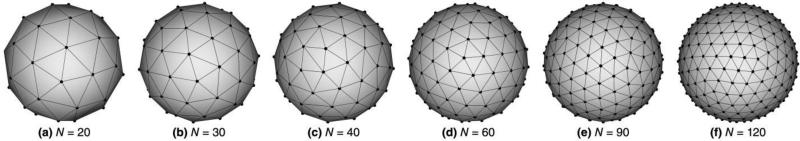
Diffusion gradient directions as vertices of a tessellated sphere used for data synthesis and analysis. In each case, the number of vertices on the sphere is twice the number of diffusion-weighting directions, N, due to the symmetry of diffusion (a measurement in direction g = [x y z]^T is equivalent to a measurement in direction –g).

For each sampling pattern, four DW data sets were generated with diffusion-weighting b = 1000 s/mm² and independent noise realization following Eq. (4), to yield SNR = 18 in the magnitude data. The SNR was chosen to match that of the invivo data set, which was estimated from the mean and standard deviation of voxels in regions of white-matter of one acquired non-DW volume. One noisy non-DW volume was simulated for every 10 DW volumes.

3.2 Data analysis

To ensure the 6 multiple-fiber analysis methods were evaluated fairly the parameters of each method were individually optimized for each of the diffusion sampling patterns, with the following objective in mind: maximize the detection of true fibers (to permit accurate assessment of the error associated with estimating multiple fibers per voxel), with limited number of false-positives (which otherwise increase spurious and false tractography). We are able to adjust parameters towards achieving this objective because the fiber ground-truth is known. Formally, the following constraints were imposed:

• i)The false-positive rate for single-fiber voxels should not exceed 10%, and be approximately equal among analysis methods and constant over all sets of diffusion-weighting directions, and
• ii)The false-positive rate for two-fiber voxels should not exceed 5%, averaged over all two-fiber crossing angles.

Following is a brief description of the software tools used for the data analysis. The final set of parameters used for analysis is listed in Table 1.

Table 1.

Summary of parameters used for data analysis.

Analysis Method	Diffusion-weighting directions
	20	30	40	60	90	120
BSM	N=3	N=3	N=3	N=3	N=3	N=3
CSD	lmax=6*	lmax=8*	lmax=8*	lmax=10*	lmax=12*	lmax=12
QBI	l=4	l=6	l=6	l=8	l=10	l=12
	λ=0.006	λ=0.006	λ=0.006	λ=0.006	λ=0.006	λ=0.006
FRACT	L=4	L=6	L=6	L=8	L=10	L=12
	λ=0.006	λ=0.006	λ=0.006	λ=0.006	λ=0.006	λ=0.006
	ξ=0.10ρ	ξ=0.40ρ	ξ=0.40ρ	ξ=0.45ρ	ξ=0.45ρ	ξ=0.45ρ
CSA	l=4	l=4	l=4	l=4	l=4	l=4
	δ1=δ2=0.01	δ1=δ2=0.01	δ1=δ2=0.01	δ1=δ2=0.01	δ1=δ2=0.01	δ1=δ2=0.01
GQI	σ=1.66	σ=1.85	σ=1.90	σ=1.95	σ=2.05	σ=2.10

Notation for parameters is summarized here: N = maximum number of fibers; l_max, l, L = maximum degree of the spherical harmonic series; λ = weighting of Laplace-Beltrami regularization term; ξ = parameter of FRACT method; δ₁, δ₂ = thresholding parameters of CSA method; σ = diffusion sampling length ratio. Refer to references of each method for notation details. The * indicates super-resolved non-negativity CSD.

Ball and Stick Model (BSM)

Using identical method as per analysis of the in-vivo data (Sect. 2.1), the FSL program ‘bedpostx’ was used for the “ball and stick” model, with default parameters for estimating up to 3 fibers per voxel.

Constrained Spherical Deconvolution (CSD)

The software package MRtrix (MRtrix v0.2.11; http://www.brain.org.au/software; Tournier et al., 2012) was used for nonnegativity constrained normal and super-resolved spherical deconvolution approaches. The order of the spherical harmonics for estimation of the single-fiber response function (‘estimate_response’ command) and spherical deconvolution (‘csdeconv’ command) steps were specified. In our analysis, super-resolved CSD was used for all but one of the diffusion gradient sampling patterns (N = 120), for which better results were obtained for our synthetic data using normal CSD.

Q-Ball Imaging (QBI)

We implemented analytical QBI reconstruction in MATLAB according to the symmetric and real-valued spherical harmonics framework proposed by (Descoteaux et al., 2007). This approach makes use of the Funk-Hecke theorem to analytically evaluate the Funk-Radon Transform (FRT) of QBI, in conjunction with Laplace-Beltrami regularization to improve robustness to noise.

Funk-Radon and Cosine Transform (FRACT)

FRACT is an alternative to the FRT used in QBI, and was readily implemented by modifying our QBI implementation; the eigenvalues used in computing the FRT were exchanged with values derived from the kernel function of FRACT. See (Haldar and Leahy, 2013) for details of the FRACT kernel and its associated spherical harmonics eigenvalues.

Constant Solid Angle QBI (CSA)

A MATLAB implementation of the CSA method was provided by Aganj for this work, and is fully described in (Aganj et al., 2010). We found it necessary to use a spherical harmonics order of 4 for all numbers of gradient directions to avoid noisy orientation distribution functions resulting in a high rate of false-positive fibers.

Generalized q-sampling Imaging (GQI)

We implemented GQI reconstruction in MATLAB as described by (Yeh et al., 2010). The optimal mean diffusion length ratio, σ, was experimentally determined; we found that values greater than those (σ = 1.0–1.3) recommended by Yeh et al. for b-values of 3000–4000 s/mm² achieved best results for our low b-value synthetic data (b = 1000 s/mm²).

Estimated fiber orientations were obtained differently depending on the analysis method. For BSM, fiber orientations were output directly by the program ‘bedpostx’. For CSD, the MRtrix command ‘find_SH_peaks’ was used to determine the orientations of up to three largest peaks of the FOD, which were in turn taken as fiber orientations. For the remaining methods a similar peak finding task was accomplished with an in-house MATLAB code by reconstructing the ODF (for QBI, FRACT or CSA) or SDF (for GQI) on a tessellated sphere having 2562 radial projections. In these cases estimated fiber orientations include an additional error of up to ~2.7°, as fibers are constrained to the orientations of these projections.

All peak detection approaches required the use of a threshold (minimum value of local maxima) to eliminate minor peaks resulting from noise, which would otherwise lead to false-positive fibers. Table 2 summarizes the threshold values used.

Table 2.

Thresholds used to eliminate minor peaks as fraction of mean value of the applicable spherical function (FOD, ODF or SDF).

Analysis Method	Diffusion-weighting directions
	20	30	40	60	90	120
CSD	0.30	0.35	0.30	0.35	0.45	0.40
QBI	0.00	0.00	0.00	0.00	0.00	0.00
FRACT	0.30	0.70	0.70	0.70	0.70	0.70
CSA	2.10	1.90	1.75	1.55	1.45	1.33
GQI	0.92	0.92	0.92	0.92	0.92	0.92

3.3 Comparison of in-vivo and synthetic data

A brief qualitative comparison of GFA, color FA, and tractography obtained from analysis of the in-vivo data and an example set of synthetic noisy data (SNR = 18) is shown in Fig. 2, which also illustrates the ‘whole-brain’ extent of our synthetic data.

Fig. 2.

Example qualitative comparison of results obtained from in-vivo data (row 1) and synthetic noisy data (SNR = 18) (row 2); both data sets consisted of 150 DW volumes and 10 non-DW volumes. The three columns are: generalized FA (left), color FA (middle) and tractography of the left cingulum (right). Corresponding images have identical intensity scales. Color in the images corresponds to orientation of the principal eigenvector in the color FA image, and local orientation of the fiber in the tractography image.

In Fig. 2 the GFA images are almost identical since GFA of the in-vivo data was approximated in computing f₀ for the synthetic data model as described in Sect. 2.1. The color FA image from the synthetic data is marginally brighter (higher FA) compared to that of the in-vivo data, particularly in regions bordering ventricles (see circles). Minor differences can be seen in tractography of the left cingulum as a result of small differences in estimated fiber orientations. Overall, the close correspondence of synthetic data results to those of in-vivo data allows us to gain confidence in our simulation framework.

3.4 Fiber orientation estimation

In the plots of Figs. 3 to 6 each data point is the mean value of the quantity indicated, wherein the average is taken over all (four) independent noise realizations and all similar voxels as categorized by the ground-truth. Only voxels satisfying the following criteria in the ground-truth were included in results: 1) voxel must be classified as WM, 2) individual fibers must have a volume fraction of at least 15%, and 3) the free-diffusion compartment size is no more than 30%. The purpose of the criteria is to filter-out voxels in which estimated fiber orientations are governed by noise, leading to random magnitude of fiber orientation error. False-positive/-negative rates are given in terms of the percentage of individual fibers in the ground-truth satisfying the criteria.

Fig. 3.

Single-fiber estimation versus number of diffusion-weighting gradient directions, N. Multi-fiber analysis method indicated by color according to the legend. Filled markers (circle and triangle) are mean values of the quantity indicated. (a) Individual fiber orientation error. (b) Corresponding false-positive rate.

Fig. 6.

Three fiber estimation versus number of diffusion-weighting gradient directions, N. Multi-fiber analysis method indicated by color according to the legend. Filled markers (circle and triangle) are mean values of the quantity indicated. (a) Individual fiber orientation error. (b) Corresponding false-negative rate.

One fiber/voxel

Fig. 3 presents the results of fiber estimation error and false-positive rate for voxels containing a single fiber. For clarity, error bars are not shown; the reader is referred to the online supplementary material for this information.

Fig. 3(a) shows that even in the simplest case of single fiber estimation, an increase in the number of DW directions helps reduce fiber orientation error, although beyond N = 60 there is minimal improvement. The BSM method had the least fiber orientation error, as would be expected because its model most closely matches that used for data synthesis, Eq. (1). The CSD method also performed very well, and this can be attributed to accurate estimation of the single-fiber response function over a large number of voxels having synthetic data modeled by identical fibers with diffusion tensor given by Eq. (3).

Fig. 3(b) shows approximately constant false-positive rate for all methods over the range of DW directions, and values are < 10% (in accordance with out constraints for parameter adjustment in Sect. 3.2). There are no false-negatives because at least one fiber orientation must be present.

Two fibers/voxel

For voxels with two-fibers, fiber estimation results are grouped according to the crossing angle (0–90°) of the two fibers in the ground truth; 9 bins of width 10° are used. Fiber orientation error and false-negative rate is shown in Fig. 4 (grouped by number of diffusion-weighing directions) and Fig. 5 (grouped by analysis method). For clarity, the false-positive rate (which never exceeds a few percent for any data point) is not shown; the reader is referred to the online supplementary data for this information.

Fig. 4.

Two fiber estimation versus fiber crossing angle; multi-fiber analysis method indicated by color according to the legend. Filled markers (circle and triangle) are mean values of the quantity indicated. (a)-(f) Individual fiber orientation error, with increasing N. (g)-(l) Corresponding false-negative rate, with increasing N.

Fig. 5.

Two fiber estimation versus fiber crossing angle; number of diffusion-weighting gradient directions indicated by color according to the legend. Filled markers (circle and triangle) are mean values of the quantity indicated. (a)-(f) Individual fiber orientation error, for each analysis method. (g)-(l) Corresponding false-negative rate, for each analysis method.

In Figs. 4 and 5 the left column of graphs illustrates individual fiber orientation error and the right column the corresponding false-negative rate, i.e. missing true fibers. For crossing angles approaching zero the false rate is often approximately −50%, indicating only half the fibers present were detected. This is as expected, as two increasingly parallel fibers eventually become indistinguishable from a single fiber.

Fig. 4 directly compares the diffusion analysis methods. As N increases there is greater differentiation between the methods in terms of both orientation error and false rate. As for voxels with single fibers, BSM and CSD perform similarly to each other, and almost always yield the least orientation error and false rate closest to zero. Once again, this is expected as both methods are positively biased due to the simulation model.

For N = 20 and 30, CSD outperforms BSM in terms of false rate for crossing angles > 45°. This was found (results not shown) to be attributed to the higher-order spherical harmonics of super-resolved CSD, that leads to improved angular resolution and consequently fiber orientation estimation, especially for low N (Tournier et al., 2007).

We found QBI typically had the largest orientation errors and greatest false-negative rate for all N. From Fig. 4(g)-(l), we see that the false rate of QBI is −50% (for all N) until the 70–80° bin, indicating that two fibers cannot be resolved below crossing angle of approximately 75°. This is consistent with the results of (Descoteaux et al., 2007), in which a crossing angle of 74° or 75° (depending on order of the spherical harmonics, L) was identified as the critical angle below which only a single maxima on the ODF starts to be detected instead of two. Several ODF sharpening techniques have been developed (Descoteaux et al., 2009, Yeh et al., 2011) to enhance maxima of the fiber orientations on the ODF, although they are not explored in this work.

Our results show that FRACT substantially improves upon the FRT used in QBI, which in part is due to FRACTs suppression of the isotropic component of the ODF, allowing anisotropic components to be more easily detected. Compared to the FRT of QBI, FRACT generally decreased the orientation error and lowered the critical angle for detection of two fibers to 55°. Furthermore, FRACT significantly increased the detection rate of two fibers; for example the false-negative rate dropped from −45% for QBI in the 70–80° crossing angle bin (N = 60) to −20% for FRACT.

Overall, we found the most defining characteristic between the methods to be the false-negative rate. Even when there is little difference in orientation error separating the methods, there can be a substantial difference in false-negative rate. For example, at N = 60 and considering the 70–80° bin, the difference in orientation error between the best and worst method is approximately 3°, whereas the corresponding difference in false-negative rate is 45%.

Fig. 5 groups the results by analysis method and in each case a clear trend of reduced orientation error and improved fiber detection is seen with increasing N. Also revealed is the unique manner in which orientation error and false rate changes with N; for some methods a limited range of fiber crossing angles benefits from increased N, whereas other methods show improvement over a wide range of crossing angles. It is clear that some methods benefit from increased N more than others.

The reader is referred to the online supplementary material for inclusion of error bars and false-positive rate.

Three fibers/voxel

In the case of three fibers per voxel, wherein each of the fibers are oriented independently of each other and effectively randomly, a single crossing angle is insufficient to describe the relative fiber orientations. However, as the true fiber orientations are known from the ground truth, we are still able to calculate the orientation error of individual estimated fibers and detect false-negatives.

Fig. 6 presents the results of fiber estimation error, and false-negative rate, for voxels containing three fibers.

Fig. 6(a) shows that N is a significant factor in reducing orientation error in the case of three fibers per voxel. Unlike the result of Fig. 3(a), there is more notable reduction in orientation error for N > 60 in this case. For N ≥ 60, there is little difference (≈1°) in orientation error between the methods.

Fig. 6(b) reveals substantial differences in detection rate of fibers between the methods, and we expect this to have significant impact on tractography through regions of crossing fibers. With the exception of GQI, all methods indicate improved detection rate of fibers with increasing N, although some methods show more substantial gains than others.

There are no false-positives in three fiber voxels because at most 3 fiber orientations were estimated by each analysis method.

The online supplementary material includes error bars for each of the methods.

3.5 Tractography and white-matter pathway differences

Whole-brain streamline tractography was performed using an in-house C program. The fiber tracking algorithm used is similar to the Euler integration scheme by Basser et al. (Basser et al., 2000), but modified to accommodate multiple fiber orientations per voxel. Track propagation used a fixed step size (0.2 mm) and at each step the propagation direction was calculated by tri-linear interpolation of fiber orientations from the eight voxels surrounding the current position. For each surrounding voxel, only the fiber orientation with smallest deflection angle (with respect to the current propagation direction) was used for interpolation. As track seeding and filtering would impact tractography results, we used a single consistent set of seed points and filtering criteria for processing all data sets. Tractography seed points (5 seeds/voxel) were distributed in all voxels classified as WM in the ground-truth, with identical seeds used in fiber tracking of all data sets. From the seed points, track propagation continued throughout a track mask consisting of all voxels classified as WM, and any other voxel having partial volume WM > 2% and CSF < 40% (based on the ground-truth tissue segmentation; see Sect. 2.1). Additional track termination criteria included: maximum change in track propagation direction between steps = 45°, and maximum track curvature = 90° over 10 mm.

Prominent white-matter pathways

Tractography of the in-vivo data was used to identify four prominent white-matter pathways for comparison: the left cingulum (C), left inferior longitudinal fasciculus (LF), right inferior fronto-occipital fasciculus (FOF), and right corticospinal track (CST), as shown in Fig. 7. The pathways were identified following procedures described by (Catani and Thiebaut de Schotten, 2008).

Fig. 7.

Four white-matter pathways identified from the in-vivo data and assumed as the ground-truth: left cingulum (red), left inferior longitudinal fasciculus (purple), right inferior fronto-occipital fasciculus (blue), and right corticospinal track (green). A registered T₁-weighted anatomical image is inserted for reference. Orientations are as indicated.

Before quantitative comparison we converted the continuous fiber paths (Fig. 7) to discrete voxelized regions (Fig. 8) by transforming fractional track coordinates to integer voxel space.

Fig. 8.

Voxelized regions of the track paths of Fig. 7. The regions are: left cingulum (red), left inferior longitudinal fasciculus (purple), right inferior fronto-occipital fasciculus (blue), and right corticospinal track (green). A registered T₁-weighted anatomical image is inserted for reference. Orientations are as indicated.

Tractography from each simulated data set was filtered with the same regions-of-interest used in obtaining the ground-truth pathways, and then voxelized. Voxelized results from each of the independent noise trials were then averaged.

For each of the four pathways we calculated the percent voxelized region found overlapping and non-overlapping its corresponding ground-truth. Example tractography and corresponding voxelized regions for each multi-fiber analysis method are shown in Fig. 9.

Fig. 9.

Tractography (columns 1 and 2) and corresponding discrete voxelized regions (columns 3 and 4) obtained from processing one N = 60 DW data set by each of the six analysis methods (individual rows). White-matter pathways are: left cingulum (red), left inferior longitudinal fasciculus (purple), right inferior fronto-occipital fasciculus (blue), and right corticospinal track (green). A registered T₁-weighted anatomical image is inserted for reference. Left and right orientation only, as indicated. Comparable tractography between methods is expected as the underlying voxels likely contain single fibers. See additional clarification in the text.

Fig. 9 shows all methods are capable of recovering these prominent white-matter pathways with only minor differences between results. This is unsurprising as the chosen track paths have relatively high fractional anisotropy throughout (mean FA of the in-vivo data for the regions in Fig. 8 is {FA^C,FA^LF,FA^FOF,FA^CST} = {0.42,0.46,0.51,0.55}) and as such a single fiber is likely to be the most appropriate model to the data. For single-fiber voxels, results from Fig. 3 indicate only a small difference in orientation error (≈1.7° at N = 60 between the best and worst methods), and no missing fibers (false-negatives) for any method, and so comparable tractography is expected.

The average percent overlap and non-overlap of voxelized regions relative to the ground-truth is given in Tables 3–6.

Table 3.

Average percentage of overlapping (v₁) and non-overlapping (v₂) voxelized tractography, written v₁/v₂, for the left cingulum relative to the ground-truth; greatest overlap for each set of diffusion-weighting directions indicated in bold.

Analysis Method	Diffusion-weighting directions, N
	20	30	40	60	90	120
BSM	63.5 / 14.2	72.5 / 13.7	69.0 / 11.5	73.0 / 16.8	75.7 / 13.9	75.9 / 14.5
CSD	60.8 / 11.8	64.7 / 14.5	67.9 / 14.3	74.4 / 22.8	74.6 / 19.5	71.1 / 13.2
QBI	58.1 / 10.0	54.6 / 8.9	61.6 / 11.5	63.5 / 12.5	64.4 / 10.4	65.0 / 7.4
FRACT	58.2 / 13.6	59.8 / 12.3	59.9 / 10.0	70.6 / 17.4	68.7 / 13.6	67.6 / 11.4
CSA	51.8 / 11.0	56.6 / 9.6	64.4 / 12.1	69.2 / 11.4	68.6 / 11.1	72.8 / 12.2
GQI	36.2 / 22.4	56.3 / 10.0	63.2 /15.1	62.8 / 18.9	66.8 / 10.9	66.0 / 8.1

Table 6.

Average percentage of overlapping (v₁) and non-overlapping (v₂) voxelized tractography, written v₁/v₂, for the right corticospinal track relative to the ground-truth; greatest overlap for each set of diffusion-weighting directions indicated in bold.

Analysis Method	Diffusion-weighting directions, N
	20	30	40	60	90	120
BSM	62.3 / 46.2	64.4 / 44.9	53.8 / 29.6	62.4 / 30.2	60.9 / 24.6	47.6 / 18.1
CSD	67.8 / 49.6	71.1 / 55.3	72.6 / 58.0	73.8 / 53.2	79.3 / 60.4	79.2 / 59.3
QBI	59.0 / 42.7	59.9 / 41.4	57.3 / 39.9	59.1 / 38.2	60.0 / 42.9	59.3 / 43.4
FRACT	66.3 / 53.2	64.8 / 51.0	66.7 / 57.0	68.5 / 49.1	73.7 / 54.0	71.2 / 49.4
CSA	68.5 / 56.0	67.2 / 44.7	65.0 / 42.8	66.5 / 41.6	71.1 / 48.3	70.8 / 46.9
GQI	49.4 / 51.5	56.8 / 40.8	64.2 / 46.7	60.7 / 41.0	66.8 / 54.1	62.1 / 42.5

Tables 3–6 show a general increase in fraction of recovered white-matter pathways with higher number of diffusion-weighting directions, for all analysis methods. This trend is generally not monotonic with N, and is in part due to the uncertain way in which changes in fiber orientation affect propagation of track paths over long distances. Overall we find that reduced fiber orientation error leads to quantitative improvement in estimation of white-matter pathways, even in the case of simple prominent white-matter pathways as shown here. Consistent with our findings of fiber orientation error, either BSM or CSD estimated fibers yielded the largest overlapping fraction of each pathway with respect to the ground-truth.

A trend in percent non-overlapping white-matter is less clear. Increasing N would assume to reduce the volume of non-overlapping incidental regions, and this can be observed in Tables 3–6 in some cases (~25%). However, in a similar number of cases the percent non-overlapping pathways increased, and the remaining cases (~50%) had no clear increase or decrease in non-overlapping region with greater N. This variability may be attributed to our ground-truth pathways which were established from the in-vivo data. While we necessarily interpret our ground-truth as definitive for the purpose of comparison, it is itself an approximation of reality with unknown accuracy. If our ground-truth regions were subsets of their respective actual pathways, the non-overlapping volumes could represent additional valid contributions to the estimated white-matter pathways. Alternatively, the non-overlapping volume may encompass a neighboring anatomically different white-matter pathway which is undesirable. Because of the ambiguity it is not possible to conclusively interpret the non-overlapping volume.

As reported in Tables 3–6 the percent non-overlapping region can be comparable to, even greater than, the percent overlapping region. This finding highlights a caveat for tractography-based region analyses: if the non-overlapping fraction is significant, it could lead to diminished or inflated measures of significant difference (e.g. t-scores) between groups.

Three-fiber white-matter crossing region

We examined tractography through a complex crossing-fiber region consisting of intersecting mediolaterally directed transcallosal fibers, vertically oriented corticospinal fibers, and anterior-posterior association fibers comprising part of the superior longitudinal fasciculus, as revealed by (Wedeen et al., 2008) using DSI. The tractography ground-truth of these pathways was recovered from the in-vivo data, as shown in Fig. 10.

Fig. 10.

Tractography from the in-vivo data through a complex fiber crossing region; intersection of callosal fibers (red), corticospinal fibers (blue) and association fibers (green). Orientation is oblique posterior view. Inset: magnified crossing region with reduced diameter fibers for clarity. A registered T₁-weighted anatomical image is inserted for reference.

While our in-vivo data was acquired with relatively low diffusion-weighting, which inherently limits the accuracy and ability to resolve individual fibers in complex crossing regions (Cho et al., 2008; Tournier et al., 2004, 2008; Tuch et al., 2004), Fig. 10 shows three unique fiber branches intersecting and successfully traversing a crossing-region, though not as comprehensively as in (Wedeen et al., 2008). In our result several corticospinal fibers can be seen terminating incorrectly in the vicinity of the crossing-region as a result of abrupt changes in estimated fiber orientations. While such shortcomings would likely have been lessened had a higher b-value (e.g. b = 1500-2000 s/mm²) been used for the in-vivo acquisition, Fig. 10 reassures that the fiber orientation ground-truth established in this work is sufficiently accurate to permit reproduction of tracks in pathways of complex fiber crossings, and is therefore suitable as a basis for comparison of multi-fiber per voxel analysis methods.

Fig. 11 illustrates the methods’ varying ability to recover each of the pathways, and their relative success of traversing the crossing region. In BSM and CSD there are a large number of tracks in each pathway and therefore evidently more voxels in the crossing region contain three fibers allowing the individual tracks to continue uninterrupted. The FRACT, CSA and GQI methods recover tracks in all three pathways, though crossing areas consist mostly of pairs of tracks and the fiber bundles themselves appear mostly adjacent to each other with few intersections. The QBI result illustrates the outcome for which a large percentage of false-negatives (missing true fiber orientations) lead to parallel fiber bundles unable to cross each other. Overall, the number of fibers propagating through the three-fiber crossing region correlates strongly with the false-negative rates reported in Fig. 6(b).

Fig. 11.

Tractography obtained from processing simulated N = 60 DW direction data by each of the six DW-MRI analysis methods showing intersection of callosal fibers (red), corticospinal fibers (blue) and association fibers (green). Orientation is oblique posterior view. Inset: magnified crossing region with reduced diameter fibers for clarity. A registered T₁-weighted anatomical image is inserted for reference.

Quantitative results of the percent overlap and non-overlap of voxelized equivalents of the callosal, corticospinal and association fiber bundles relative to the ground-truth is presented in Tables 7–9, respectively.

Table 7.

Average percentage of overlapping (v₁) and non-overlapping (v₂) voxelized tractography, written v₁/v₂, for the mediolateral transcallosal fibers relative to the ground-truth; greatest overlap for each set of diffusion-weighting directions indicated in bold.

Analysis Method	Diffusion-weighting directions, N
	20	30	40	60	90	120
BSM	53.5 / 63.3	53.9 / 66.1	59.4 / 70.4	67.3 / 78.3	68.3 / 82.0	66.4 / 60.0
CSD	60.7 / 72.7	68.0 / 82.7	64.0 / 76.3	71.6 / 87.4	67.3 / 82.6	75.3 / 80.0
QBI	47.2 / 57.7	48.8 / 60.2	48.3 / 65.3	52.9 / 63.0	55.0 / 72.2	54.5 / 71.3
FRACT	54.7 / 71.1	60.3 / 76.0	53.7 / 77.3	62.4 / 79.6	63.2 / 79.9	64.9 / 85.3
CSA	51.8 / 56.1	54.4 / 73.3	58.5 / 78.1	65.3 / 84.6	66.9 / 85.9	65.5 / 86.6
GQI	32.9 / 29.7	41.2 / 49.6	47.3 / 63.4	62.3 / 79.2	61.0 / 79.4	62.0 / 78.1

Table 9.

Average percentage of overlapping (v₁) and non-overlapping (v₂) voxelized tractography, written v₁/v₂, for the anterior-posterior association fibers relative to the ground-truth; greatest overlap for each set of diffusion-weighting directions indicated in bold.

Analysis Method	Diffusion-weighting directions, N
	20	30	40	60	90	120
BSM	3.8 / 1.3	5.9 / 1.3	13.1 / 2.8	14.9 / 1.8	32.4 / 11.2	41.9 / 8.0
CSD	17.2 / 5.3	35.6 / 15.3	33.3 / 10.9	54.8 / 20.2	62.3 / 31.3	65.9 / 27.5
QBI	0.0 / 0.0	0.0 / 0.0	0.0 / 0.0	0.0 / 0.0	0.0 / 0.0	0.0 / 0.0
FRACT	4.1 / 0.6	9.0 / 5.9	15.6 / 5.8	27.3 / 12.6	25.1 / 9.1	19.8 / 8.7
CSA	0.0 / 0.0	5.8 / 4.4	2.5 / 1.3	19.2 / 6.0	13.4 / 1.4	26.8 / 5.5
GQI	0.0 / 0.0	3.0 / 1.5	4.5 / 1.8	7.6 / 3.1	3.0 / 0.0	24.8 / 9.0

Tables 7–9 yield similar conclusions as to the effect of the number of diffusion-weighting directions on the overlapping and non-overlapping fraction of recovered pathways as was observed in Tables 3–6. It is unexpected that results in Tables 6 and 8, both regarding the corticospinal track, show BSM to have a decreasing trend in overlapping region as N increases. These pair of results is opposite of other methods’ and we are unable to rationalize this result.

Table 8.

Average percentage of overlapping (v₁) and non-overlapping (v₂) voxelized tractography, written v₁/v₂, for the vertically oriented corticospinal track fiber relative to the ground-truth; greatest overlap for each set of diffusion-weighting directions indicated in bold.

Analysis Method	Diffusion-weighting directions, N
	20	30	40	60	90	120
BSM	80.6 / 128.3	80.2 / 113.8	68.0 / 68.7	63.9 / 44.6	64.0 / 41.7	56.6 / 27.8
CSD	82.0 / 122.1	85.0 / 118.6	83.0 / 122.0	82.5 / 107.8	86.3 / 117.3	87.6 / 105.0
QBI	78.0 / 128.3	77.5 / 121.3	78.5 / 125.4	79.2 / 121.8	80.8 / 131.3	82.2 / 135.8
FRACT	83.4 / 139.8	84.0 / 133.2	85.4 / 146.0	84.9 / 129.3	88.0 / 139.2	86.6 / 127.8
CSA	81.3 / 134.2	85.7 / 109.9	82.0 / 107.5	83.5 / 113.4	86.7 / 137.7	86.0 / 129.5
GQI	56.6 / 119.1	75.1 / 124.1	80.8 / 125.6	80.3 / 114.2	85.7 / 143.5	83.0 / 125.3

Overall the three-fiber crossing emphasizes the importance of accurate estimation of all present fiber orientations present in order to recover track paths through complex fiber crossing regions.

4. Conclusion

Diffusion-weighted MRI uniquely has the potential to reveal the human brain's white-matter connectivity in-vivo, and as such it is being enthusiastically applied to a broad range of problems in neuroscience and clinical research. As the field has matured, advances in diffusion signal modeling and analysis has led to many alternative diffusion sampling strategies and analysis methodologies. For the researcher, it can be difficult to choose the optimal method for analyzing their data from the alternatives available.

In this work we conducted a simulation study to evaluate six multiple-fiber diffusion MRI analysis methods at a diffusion-weighting and SNR common to clinical settings. We focused on issues relevant to white-matter tractography and quantitatively compared the methods in terms of estimated fiber orientation error, false-positive and false-negative fibers, and percent recovery of select white-matter pathways. A range of diffusion-weighting directions, N, were investigated to analyze the effect of angular sampling. To ensure findings were as relevant as possible to practical application, we developed the simulation from an in-vivo data set.

Of the methods studied, and within the scope of clinically acquired diffusion data (b ≈ 1000 s/mm² and SNR ≈ 18), we found the two-compartment “ball and stick” model (BSM) and non-negativity constrained super-resolved spherical deconvolution (CSD) methods yielded the most accurate fiber orientation estimation, and greatest detection rate of fibers, for all N. Additionally we observed that even small improvements in fiber estimation, in terms of both reduced orientation error and greater detection rate, engendered more complete recovery of white-matter pathways via tractography. While all methods were able to recover prominent white-matter pathways consisting of generally high FA and therefore minimal crossing of fibers, a complex three-fiber crossing region revealed significant differences. For the particular region studied we found fiber orientations estimated by CSD led to a substantially greater number of tracks able to traverse the crossing region than the alternative approaches. This outcome can be attributed to the much higher detection rate of fibers achieved by CSD, particularly for voxels containing three fibers.

We wish to emphasize that our investigation focused on DW data typical of clinical neuro-radiological settings, for which diffusion-weighting b ≈ 1000 s/mm² and SNR ≈ 18 are common. The relatively low b-value is not equally suited to all the analysis methods we studied, and as such the results presented will invariably be lower than could be obtained with individually optimal data acquisition. At high b values (b ≳ 1500 s/mm²) the relative fiber estimation performance of the methods studied may be notably different.

We acknowledge the BSM and CSD methods are favorably biased in comparison to the remaining approaches due to the data synthesis model, which is based on rotating a single fiber represented by a tensor. Also, the BSM and CSD methods used their own algorithms to estimate fiber orientations, which are different to the discrete peak-finding technique we implemented for QBI, FRACT, CSA and GQI. The extent of bias in the BSM and CSD results could be evaluated by using more generalized methods for data synthesis; for example, a taxonomy of multi-compartment models of white-matter comprising intra- and extra-cellular water (Panagiotaki et al., 2012), or Monte-Carlo random-walk simulations using three-dimensional mesh substrates to model complex diffusion environments (Hall et al., 2009; Panagiotaki et al., 2010).

Another limitation of this work is that we use the same single-fiber tensor model, D_x, throughout the brain. In future work it would be desirable to use tract or region specific D_x, especially as it would reduce bias to the BSM and CSD methods. We did not try this here, however. For tract/region specific D_x to contribute to a more accurate brain-like phantom, its variation throughout the brain would have to be accurately established, otherwise it may undermine the desired improved quality of the simulation. For example, loss of continuity of long fiber tracts when performing tractography may result. In the present case we do not believe the raw data (a single acquisition of a single subject) used for developing the ground-truth of fiber directions and estimating the single D_x would be sufficient for accurate estimation of tract/region specific D_x.

Our results provide important information on the performance of fiber estimation and subsequent tractography for a set of well-known diffusion analysis methods and sampling patterns. We believe the results to be of particular interest to researchers undertaking tractography-based analyses and brain network/connectivity studies. To encourage evaluation of more recent DW-MRI analysis methods, and permit exploring specific applications in clinical or research settings, we have made the data sets (which include three SNR values, 10 noise realizations, and 6 diffusion sampling patterns) and quantitative tools developed in this research publicly available via the NITRC project “Simulated DW-MRI Brain Data Sets for Quantitative Evaluation of Estimated Fiber Orientations” at http://www.nitrc.org/projects/sim_dwi_brain. It is our hope these tools are found valuable to the community towards development of not just more, but better, DW-MRI analysis methods.

Highlights.

• ■ Development of simulated diffusion-weighted brain images based on in-vivo data.

• ■ Improvements in fiber estimation engendered more complete white-matter pathways.

• ■ Accurate fiber estimation essential to tractography through complex crossing-regions.

• ■ Of the methods evaluated, non-negativity constrained super-resolved spherical deconvolution yielded best results on clinical diffusion-weighted data.

Table 4.

Average percentage of overlapping (v₁) and non-overlapping (v₂) voxelized tractography, written v₁/v₂, for the left inferior longitudinal fasciculus relative to the ground-truth; greatest overlap for each set of diffusion-weighting directions indicated in bold.

Analysis Method	Diffusion-weighting directions, N
	20	30	40	60	90	120
BSM	68.6 / 65.2	76.9 / 54.7	75.6 / 40.2	78.8 / 47.3	82.0 / 33.9	84.1 / 36.4
CSD	73.0 / 70.8	77.7 / 74.0	76.8 / 56.5	85.3 / 85.5	82.6 / 60.3	87.3 / 82.9
QBI	60.5 / 57.4	63.5 / 62.9	65.0 / 59.7	64.8 / 56.0	64.5 / 63.3	63.9 / 26.1
FRACT	65.9 / 70.5	65.6 / 58.5	75.4 / 66.3	71.0 / 59.6	71.4 / 68.4	73.0 / 70.7
CSA	64.5 / 54.7	65.9 / 49.1	70.8 / 41.8	72.8 / 59.5	71.6 / 49.2	74.6 / 56.4
GQI	58.0 / 48.9	57.9 / 55.9	70.2 / 67.4	66.3 / 69.9	67.6 / 59.8	67.5 / 69.0

Table 5.

Average percentage of overlapping (v₁) and non-overlapping (v₂) voxelized tractography, written v₁/v₂, for the right inferior fronto-occipital fasciculus relative to the ground-truth; greatest overlap for each set of diffusion-weighting directions indicated in bold.

Analysis Method	Diffusion-weighting directions, N
	20	30	40	60	90	120
BSM	75.0 / 90.1	78.9 / 74.6	78.9 / 56.9	76.6 / 50.4	81.7 / 39.1	79.9 / 38.5
CSD	76.8 / 59.3	76.8 / 63.2	78.8 / 63.4	81.1 / 66.0	84.8 / 83.7	82.1 / 62.9
QBI	69.3 / 86.6	71.1 / 99.0	73.5 / 92.5	73.8 / 87.8	72.9 / 87.7	73.8 / 86.8
FRACT	68.1 / 69.8	70.0 / 70.9	75.1 / 67.8	75.1 / 71.4	72.1 / 61.4	75.7 / 76.8
CSA	68.9 / 51.5	65.0 / 52.1	74.3 / 51.0	70.2 / 53.4	70.8 / 47.8	75.8 / 59.7
GQI	25.4 / 27.9	50.4 / 32.0	79.3 / 74.5	67.7 / 58.7	76.6 / 75.0	71.3 / 55.9

References

- Aganj I, Lenglet C, Sapiro G, Yacoub E, Ugurbil K, Harel N. Reconstruction of the orientation distribution function in single-and multiple-shell q-ball imaging within constant solid angle. Magnetic Resonance in Medicine. 2010;64(2):554–566. doi: 10.1002/mrm.22365. [DOI] [PMC free article] [PubMed] [Google Scholar]
- Alexander AL, Hasan KM, Lazar M, Tsuruda JS, Parker DL. Analysis of partial volume effects in diffusion-tensor MRI. Magnetic Resonance in Medicine. 2001;45(5):770–780. doi: 10.1002/mrm.1105. [DOI] [PubMed] [Google Scholar]
- Alexander DC, Barker GJ, Arridge SR. Detection and modeling of non-Gaussian apparent diffusion coefficient profiles in human brain data. Magnetic Resonance in Medicine. 2002;48(2):331–340. doi: 10.1002/mrm.10209. [DOI] [PubMed] [Google Scholar]
- Assemlal HE, Tschumperlé D, Brun L, Siddiqi K. Recent advances in diffusion MRI modeling: Angular and radial reconstruction. Medical Image Analysis. 2011;15(4):369–396. doi: 10.1016/j.media.2011.02.002. [DOI] [PubMed] [Google Scholar]
- Basser PJ, Mattiello J, LeBihan D. MR diffusion tensor spectroscopy and imaging. Biophysical Journal. 1994a;66(1):259–267. doi: 10.1016/S0006-3495(94)80775-1. [DOI] [PMC free article] [PubMed] [Google Scholar]
- Basser PJ, Mattiello J, LeBihan D. Estimation of the Effective Self-Diffusion Tensor from the NMR Spin Echo. Journal of Magnetic Resonance, Series B. 1994b;103(3):247–254. doi: 10.1006/jmrb.1994.1037. [DOI] [PubMed] [Google Scholar]
- Basser PJ, Pierpaoli C. Microstructural and Physiological Features of Tissues Elucidated by Quantitative-Diffusion-Tensor MRI. Journal of Magnetic Resonance, Series B. 1996;111(3):209–219. doi: 10.1006/jmrb.1996.0086. [DOI] [PubMed] [Google Scholar]
- Basser PJ, Pajevic S, Pierpaoli C, Duda J, Aldroubi A. In vivo fiber tractography using DT-MRI data. Magnetic Resonance in Medicine. 2000;44(4):625–632. doi: 10.1002/1522-2594(200010)44:4<625::aid-mrm17>3.0.co;2-o. [DOI] [PubMed] [Google Scholar]
- Bastiani M, Shah NJ, Goebel R, Roebroeck A. Human cortical connectome reconstruction from diffusion weighted MRI: the effect of tractography algorithm. NeuroImage. 2012;62(3):1732–1749. doi: 10.1016/j.neuroimage.2012.06.002. [DOI] [PubMed] [Google Scholar]
- Beaulieu C. The basis of anisotropic water diffusion in the nervous system–a technical review. NMR in Biomedicine. 2002;15(7-8):435–455. doi: 10.1002/nbm.782. [DOI] [PubMed] [Google Scholar]
- Behrens TEJ, Woolrich MW, Jenkinson M, Johansen-Berg H, Nunes RG, Clare S, Matthews PM, Brady JM, Smith SM. Characterization and propagation of uncertainty in diffusion-weighted MR imaging. Magnetic Resonance in Medicine. 2003;50(5):1077–1088. doi: 10.1002/mrm.10609. [DOI] [PubMed] [Google Scholar]
- Behrens TEJ, Berg HJ, Jbabdi S, Rushworth MFS, Woolrich MW. Probabilistic diffusion tractography with multiple fibre orientations: What can we gain?. NeuroImage. 2007;34(1):144–155. doi: 10.1016/j.neuroimage.2006.09.018. [DOI] [PMC free article] [PubMed] [Google Scholar]
- Bullmore E, Sporns O. Complex brain networks: graph theoretical analysis of structural and functional systems. Nature Reviews Neuroscience. 2009;10(3):186–198. doi: 10.1038/nrn2575. [DOI] [PubMed] [Google Scholar]
- Campbell JS, Siddiqi K, Rymar VV, Sadikot AF, Pike GB. Flow-based fiber tracking with diffusion tensor and q-ball data: validation and comparison to principal diffusion direction techniques. NeuroImage. 2005;27(4):725–736. doi: 10.1016/j.neuroimage.2005.05.014. [DOI] [PubMed] [Google Scholar]
- Canales-Rodríguez EJ, Melie-García L, Iturria-Medina Y. Mathematical description of q-space in spherical coordinates: Exact q-ball imaging. Magnetic Resonance in Medicine. 2009;61(6):1350–1367. doi: 10.1002/mrm.21917. [DOI] [PubMed] [Google Scholar]
- Canales-Rodríguez EJ, Lin CP, Iturria-Medina Y, Yeh CH, Cho KH, Melie-García L. Diffusion orientation transform revisited. NeuroImage. 2010;49(2):1326–1339. doi: 10.1016/j.neuroimage.2009.09.067. [DOI] [PubMed] [Google Scholar]
- Catani M, Thiebaut de Schotten M. A diffusion tensor imaging tractography atlas for virtual in vivo dissections. Cortex. 2008;44(8):1105–1132. doi: 10.1016/j.cortex.2008.05.004. [DOI] [PubMed] [Google Scholar]
- Catani M, Dell'Acqua F, Thiebaut de Schotten M. A revised limbic system model for memory, emotion and behaviour. Neuroscience & Biobehavioral Reviews. 2013;37(8):1724–1737. doi: 10.1016/j.neubiorev.2013.07.001. [DOI] [PubMed] [Google Scholar]
- Cheng H, Wang Y, Sheng J, Sporns O, Kronenberger WG, Mathews VP, Hummer TA, Saykin AJ. Optimization of seed density in DTI tractography for structural networks. Journal of Neuroscience Methods. 2012;203(1):264–272. doi: 10.1016/j.jneumeth.2011.09.021. [DOI] [PMC free article] [PubMed] [Google Scholar]
- Cho KH, Yeh CH, Tournier JD, Chao YP, Chen JH, Lin CP. Evaluation of the accuracy and angular resolution of q-ball imaging. NeuroImage. 2008;42(1):262–271. doi: 10.1016/j.neuroimage.2008.03.053. [DOI] [PubMed] [Google Scholar]
- Côté MA, Girard G, Boré A, Garyfallidis E, Houde JC, Descoteaux M. Tractometer: Towards Validation of Tractography Pipelines. Medical Image Analysis. 2013;17(7):844–857. doi: 10.1016/j.media.2013.03.009. [DOI] [PubMed] [Google Scholar]
- Conturo TE, Lori NF, Cull TS, Akbudak E, Snyder AZ, Shimony JS, McKinstry RC, Burton H, Raichle ME. Tracking neuronal fiber pathways in the living human brain. Proceedings of the National Academy of Sciences. 1999;96(18):10422–10427. doi: 10.1073/pnas.96.18.10422. [DOI] [PMC free article] [PubMed] [Google Scholar]
- Cook PA, Bai Y, Nedjati-Gilani S, Seunarine KK, Hall MG, Parker GJ, Alexander DC. Camino: Open-Source Diffusion-MRI Reconstruction and Processing. Proc. Intl. Soc. Mag. Reson. Med. 2006;14 [Google Scholar]
- Cook PA, Symms M, Boulby PA, Alexander DC. Optimal acquisition orders of diffusion-weighted MRI measurements. Journal of Magnetic Resonance Imaging. 2007;25(5):1051–1058. doi: 10.1002/jmri.20905. [DOI] [PubMed] [Google Scholar]
- Daducci A, Canales-Rodríguez EJ, Descoteaux M, Garyfallidis E, Gur Y, Lin YC, Ramirez-Manzanares A. Quantitative comparison of reconstruction methods for intra-voxel fiber recovery from diffusion MRI. IEEE Transactions on Medical Imaging. 2013 doi: 10.1109/TMI.2013.2285500. in press. [DOI] [PubMed] [Google Scholar]
- Dell'Acqua F, Scifo P, Rizzo G, Catani M, Simmons A, Scotti G, Fazio F. A modified damped Richardson–Lucy algorithm to reduce isotropic background effects in spherical deconvolution. NeuroImage. 2010;49(2):1446–1458. doi: 10.1016/j.neuroimage.2009.09.033. [DOI] [PubMed] [Google Scholar]
- Descoteaux M, Angelino E, Fitzgibbons S, Deriche R. Regularized, fast, and robust analytical Q-ball imaging. Magnetic Resonance in Medicine. 2007;58(3):497–510. doi: 10.1002/mrm.21277. [DOI] [PubMed] [Google Scholar]
- Descoteaux M, Deriche R, Knosche TR, Anwander A. Deterministic and probabilistic tractography based on complex fibre orientation distributions. IEEE Transactions on Medical Imaging. 2009;28(2):269–286. doi: 10.1109/TMI.2008.2004424. [DOI] [PubMed] [Google Scholar]
- Farrher E, Kaffanke J, Celik AA, Stöcker T, Grinberg F, Shah NJ. Novel multisection design of anisotropic diffusion phantoms. Journal of Magnetic Resonance Imaging. 2012;30(4):518–526. doi: 10.1016/j.mri.2011.12.012. [DOI] [PubMed] [Google Scholar]
- Fillard P, Descoteaux M, Goh A, Gouttard S, Jeurissen B, Malcolm J, Ramirez-Manzanares A, Poupon C. Quantitative evaluation of 10 tractography algorithms on a realistic diffusion MR phantom. NeuroImage. 2011;56(1):220–234. doi: 10.1016/j.neuroimage.2011.01.032. [DOI] [PubMed] [Google Scholar]
- Frank LR. Anisotropy in high angular resolution diffusion-weighted MRI. Magnetic Resonance in Medicine. 2001;45(6):935–939. doi: 10.1002/mrm.1125. [DOI] [PubMed] [Google Scholar]
- Friston K, Ashburner J, Frith CD, Poline JB, Heather JD, Frackowiak RS. Spatial registration and normalization of images. Human brain mapping. 1995;3(3):165–189. [Google Scholar]
- Gigandet X, Griffa A, Kober T, Daducci A, Gilbert G, Connelly A, Krueger G. A Connectome-Based Comparison of Diffusion MRI Schemes. PloS one. 2013;8(9):e75061. doi: 10.1371/journal.pone.0075061. [DOI] [PMC free article] [PubMed] [Google Scholar]
- Golby AJ, Kindlmann G, Norton I, Yarmarkovich A, Pieper S, Kikinis R. Interactive diffusion tensor tractography visualization for neurosurgical planning. Neurosurgery. 2011;68(2):496–505. doi: 10.1227/NEU.0b013e3182061ebb. [DOI] [PMC free article] [PubMed] [Google Scholar]
- Gudbjartsson H, Patz S. The Rician distribution of noisy MRI data. Magnetic Resonance in Medicine. 1995;34(6):910–914. doi: 10.1002/mrm.1910340618. [DOI] [PMC free article] [PubMed] [Google Scholar]
- Haldar JP, Leahy RM. Linear transforms for Fourier data on the sphere: Application to high angular resolution diffusion MRI of the brain. NeuroImage. 2013;71:233–247. doi: 10.1016/j.neuroimage.2013.01.022. [DOI] [PMC free article] [PubMed] [Google Scholar]
- Hall MG, Alexander DC. Convergence and parameter choice for Monte-Carlo simulations of diffusion MRI. IEEE Transactions on Medical Imaging. 2009;28(9):1354–1364. doi: 10.1109/TMI.2009.2015756. [DOI] [PubMed] [Google Scholar]
- Hess CP, Mukherjee P, Han ET, Xu D, Vigneron DB. Q-ball reconstruction of multimodal fiber orientations using the spherical harmonic basis. Magnetic Resonance in Medicine. 2006;56(1):104–117. doi: 10.1002/mrm.20931. [DOI] [PubMed] [Google Scholar]
- Javad F, Warren JD, Micallef C, Thornton JS, Golay X, Yousry T, Mancini L. Auditory tracts identified with combined fMRI and diffusion tractography. NeuroImage. 2014;84:562–574. doi: 10.1016/j.neuroimage.2013.09.007. [DOI] [PMC free article] [PubMed] [Google Scholar]
- Jones DK. The effect of gradient sampling schemes on measures derived from diffusion tensor MRI: a Monte Carlo study. Magnetic Resonance in Medicine. 2004;51(4):807–815. doi: 10.1002/mrm.20033. [DOI] [PubMed] [Google Scholar]
- Kuo LW, Chiang WY, Yeh FC, Wedeen VJ, Tseng WY. Diffusion spectrum MRI using body-centered-cubic and half-sphere sampling schemes. Journal of Neuroscience Methods. 2013;212(1):143–155. doi: 10.1016/j.jneumeth.2012.09.028. [DOI] [PubMed] [Google Scholar]
- LeBihan D, Breton E, Lallemand D, Grenier P, Cabanis E, Laval-Jeantet M. MR imaging of intravoxel incoherent motions: application to diffusion and perfusion in neurologic disorders. Radiology. 1986;161(2):401–407. doi: 10.1148/radiology.161.2.3763909. [DOI] [PubMed] [Google Scholar]
- Mesaros S, Rocca MA, Kacar K, Kostic J, Copetti M, Stosic-Opincal T, Filippi M. Diffusion tensor MRI tractography and cognitive impairment in multiple sclerosis. Neurology. 2012;78(13):969–975. doi: 10.1212/WNL.0b013e31824d5859. [DOI] [PubMed] [Google Scholar]
- Michailovich O, Rathi Y. On approximation of orientation distributions by means of spherical ridgelets. IEEE Transactions on Image Processing. 2010;19(2):461–477. doi: 10.1109/TIP.2009.2035886. [DOI] [PMC free article] [PubMed] [Google Scholar]
- Mori S, Crain BJ, Chacko VP, Van Zijl P. Three-dimensional tracking of axonal projections in the brain by magnetic resonance imaging. Annals of Neurology. 1999;45(2):265–269. doi: 10.1002/1531-8249(199902)45:2<265::aid-ana21>3.0.co;2-3. [DOI] [PubMed] [Google Scholar]
- Mori S, van Zijl P. Fiber tracking: principles and strategies–a technical review. NMR in Biomedicine. 2002;15(7-8):468–480. doi: 10.1002/nbm.781. [DOI] [PubMed] [Google Scholar]
- Morikawa M, Kiuchi K, Taoka T, Nagauchi K, Kichikawa K, Kishimoto T. Uncinate fasciculus-correlated cognition in Alzheimer's disease: a diffusion tensor imaging study by tractography. Psychogeriatrics. 2010;10(1):15–20. doi: 10.1111/j.1479-8301.2010.00312.x. [DOI] [PubMed] [Google Scholar]
- Moussavi-Biugui A, Stieltjes B, Fritzsche K, Semmler W, Laun FB. Novel spherical phantoms for Q-ball imaging under in vivo conditions. Magnetic Resonance in Medicine. 2011;65(1):190–194. doi: 10.1002/mrm.22602. [DOI] [PubMed] [Google Scholar]
- Panagiotaki E, Hall MG, Zhang H, Siow B, Lythgoe MF, Alexander DC. High-fidelity meshes from tissue samples for diffusion MRI simulations. In Medical Image Computing and Computer-Assisted Intervention–MICCAI. 2010;2010:404–411. doi: 10.1007/978-3-642-15745-5_50. [DOI] [PubMed] [Google Scholar]
- Panagiotaki E, Schneider T, Siow B, Hall MG, Lythgoe MF, Alexander DC. Compartment models of the diffusion MR signal in brain white matter: a taxonomy and comparison. NeuroImage. 2012;59(3):2241–2254. doi: 10.1016/j.neuroimage.2011.09.081. [DOI] [PubMed] [Google Scholar]
- Perrin M, Poupon C, Rieul B, Leroux P, Constantinesco A, Mangin JF, LeBihan D. Validation of q-ball imaging with a diffusion fibre-crossing phantom on a clinical scanner. Philosophical Transactions of the Royal Society B: Biological Sciences. 2005;360(1457):881–891. doi: 10.1098/rstb.2005.1650. [DOI] [PMC free article] [PubMed] [Google Scholar]
- Poupon C, Rieul B, Kezele I, Perrin M, Poupon F, Mangin JF. New diffusion phantoms dedicated to the study and validation of high-angular-resolution diffusion imaging (HARDI) models. Magnetic Resonance in Medicine. 2008;60(6):1276–1283. doi: 10.1002/mrm.21789. [DOI] [PubMed] [Google Scholar]
- Poupon C, Laribiere L, Tournier G, Bernard J, Fournier D, Fillard P, Descoteaux M, Mangin J-F. A diffusion hardware phantom looking like a coronal brain slice. Proc. Intl. Soc. Mag. Reson. Med. 2010;18 [Google Scholar]
- Pullens P, Roebroeck A, Goebel R. Ground truth hardware phantoms for validation of diffusion-weighted MRI applications. Journal of Magnetic Resonance Imaging. 2010;32(2):482–488. doi: 10.1002/jmri.22243. [DOI] [PubMed] [Google Scholar]
- Ramirez-Manzanares A, Cook PA, Hall M, Ashtari M, Gee JC. Resolving axon fiber crossings at clinical b-values: An evaluation study. Medical Physics. 2011;38:5239–5253. doi: 10.1118/1.3626571. [DOI] [PubMed] [Google Scholar]
- Smith SM, Jenkinson M, Woolrich MW, Beckmann CF, Behrens TE, Johansen-Berg H, Matthews PM. Advances in functional and structural MR image analysis and implementation as FSL. NeuroImage. 2004;23:S208–S219. doi: 10.1016/j.neuroimage.2004.07.051. [DOI] [PubMed] [Google Scholar]
- Toga AW, Clark KA, Thompson PM, Shattuck DW, Van Horn JD. Mapping the human connectome. Neurosurgery. 2012;71(1):1–5. doi: 10.1227/NEU.0b013e318258e9ff. [DOI] [PMC free article] [PubMed] [Google Scholar]
- Tournier J, Calamante F, Gadian DG, Connelly A. Direct estimation of the fiber orientation density function from diffusion-weighted MRI data using spherical deconvolution. NeuroImage. 2004;23(3):1176–1185. doi: 10.1016/j.neuroimage.2004.07.037. [DOI] [PubMed] [Google Scholar]
- Tournier J, Calamante F, Connelly A. Robust determination of the fibre orientation distribution in diffusion MRI: non-negativity constrained super-resolved spherical deconvolution. NeuroImage. 2007;35(4):1459–1472. doi: 10.1016/j.neuroimage.2007.02.016. [DOI] [PubMed] [Google Scholar]
- Tournier J, Yeh CH, Calamante F, Cho KH, Connelly A, Lin CP. Resolving crossing fibres using constrained spherical deconvolution: validation using diffusion-weighted imaging phantom data. NeuroImage. 2008;42(2):617–625. doi: 10.1016/j.neuroimage.2008.05.002. [DOI] [PubMed] [Google Scholar]
- Tournier J, Calamante F, Connelly A. MRtrix: Diffusion tractography in crossing fiber regions. International Journal of Imaging Systems and Technology. 2012;22(1):53–66. [Google Scholar]
- Tuch DS, Reese TG, Wiegell MR, Makris N, Belliveau JW, Wedeen VJ. High angular resolution diffusion imaging reveals intravoxel white matter fiber heterogeneity. Magnetic Resonance in Medicine. 2002;48(4):577–582. doi: 10.1002/mrm.10268. [DOI] [PubMed] [Google Scholar]
- Tuch DS, Reese TG, Wiegell MR, Wedeen VJ. Diffusion MRI of complex neural architecture. Neuron. 2003;40(5):885–895. doi: 10.1016/s0896-6273(03)00758-x. [DOI] [PubMed] [Google Scholar]
- Tuch DS. Q-ball imaging. Magnetic Resonance in Medicine. 2004;52(6):1358–1372. doi: 10.1002/mrm.20279. [DOI] [PubMed] [Google Scholar]
- Vlastarakos PV, Nikolopoulos TP, Pappas S, Buchanan MA, Bewick J, Kandiloros D. Cochlear implantation update: contemporary preoperative imaging and future prospects-the dual modality approach as a standard of care. Expert review of medical devices. 2010;7(4):555–567. doi: 10.1586/erd.10.28. [DOI] [PubMed] [Google Scholar]
- Voineskos AN, Lobaugh NJ, Bouix S, Rajji TK, Miranda D, Kennedy JL, Shenton ME. Diffusion tensor tractography findings in schizophrenia across the adult lifespan. Brain. 2010;133(5):1494–1504. doi: 10.1093/brain/awq040. [DOI] [PMC free article] [PubMed] [Google Scholar]
- Wang R, Benner T, Sorensen AG, Wedeen VJ. Diffusion Toolkit: A Software Package for Diffusion Imaging Data Processing and Tractography. Proc. Intl. Soc. Mag. Reson. Med. 2007;15 [Google Scholar]
- Wedeen VJ, Hagmann P, Tseng WYI, Reese TG, Weisskoff RM. Mapping complex tissue architecture with diffusion spectrum magnetic resonance imaging. Magnetic Resonance in Medicine. 2005;54(6):1377–1386. doi: 10.1002/mrm.20642. [DOI] [PubMed] [Google Scholar]
- Wedeen VJ, Wang RP, Schmahmann JD, Benner T, Tseng WYI, Dai G, de Crespigny AJ. Diffusion spectrum magnetic resonance imaging (DSI) tractography of crossing fibers. NeuroImage. 2008;41(4):1267–1277. doi: 10.1016/j.neuroimage.2008.03.036. [DOI] [PubMed] [Google Scholar]
- Yeh CH, Cho KH, Lin HC, Wang JJ, Lin CP. Reduced encoding diffusion spectrum imaging implemented with a bi-Gaussian model. IEEE Transactions on Medical Imaging. 2008;27(10):1415–1424. doi: 10.1109/TMI.2008.922189. [DOI] [PubMed] [Google Scholar]
- Yeh FC, Wedeen VJ, Tseng WYI. Generalized q-sampling imaging. IEEE Transactions on Medical Imaging. 2010;29(9):1626–1635. doi: 10.1109/TMI.2010.2045126. [DOI] [PubMed] [Google Scholar]
- Yeh FC, Wedeen VJ, Tseng WYI. Estimation of fiber orientation and spin density distribution by diffusion deconvolution. NeuroImage. 2011;55(3):1054–1062. doi: 10.1016/j.neuroimage.2010.11.087. [DOI] [PubMed] [Google Scholar]
Associated Data
This section collects any data citations, data availability statements, or supplementary materials included in this article.