Varying levels of complexity in transcription factor binding motifs

Abstract

Binding of transcription factors to DNA is one of the keystones of gene regulation. The existence of statistical dependencies between binding site positions is widely accepted, while their relevance for computational predictions has been debated. Building probabilistic models of binding sites that may capture dependencies is still challenging, since the most successful motif discovery approaches require numerical optimization techniques, which are not suited for selecting dependency structures. To overcome this issue, we propose sparse local inhomogeneous mixture (Slim) models that combine putative dependency structures in a weighted manner allowing for numerical optimization of dependency structure and model parameters simultaneously. We find that Slim models yield a substantially better prediction performance than previous models on genomic context protein binding microarray data sets and on ChIP-seq data sets. To elucidate the reasons for the improved performance, we develop dependency logos, which allow for visual inspection of dependency structures within binding sites. We find that the dependency structures discovered by Slim models are highly diverse and highly transcription factor-specific, which emphasizes the need for flexible dependency models. The observed dependency structures range from broad heterogeneities to sparse dependencies between neighboring and non-neighboring binding site positions.

INTRODUCTION

Transcriptional regulation mediated by transcription factors binding to genomic DNA is one of the fundamental regulatory steps of gene expression. Most transcription factors bind to regulatory segments, termed transcription factor binding sites. The binding specificity of these factors has been modeled as sequence motifs. Over the last years, the importance of dependencies between different positions of such transcription factor binding sites has been debated controversially (1–3). Several publications argue that binding energies between transcription factors and DNA are—with a few notable exceptions—largely additive across positions and thus can be captured by simple weight matrices with appropriately determined parameters (2,4–6). Others find that dependencies between binding site positions exist (7) and that including dependencies into motif models can indeed increase the performance of computational predictions of transcription factor binding sites (8–16). While dependencies between neighboring positions could be explained by DNA shape (17–19), reasons for non-neighboring dependencies are less clear.

In this paper, we aim at providing new insights into the importance of dependencies in transcription factor binding sites and investigate the diverse sources of such dependencies in a large-scale study on in vitro genomic context protein binding microarray (gcPBM) data (12,20) and in vivo ChIP-seq data from the ENCODE project (21). For this purpose, we propose a new class of probabilistic models that allow for learning dependencies between binding site positions discriminatively, which we call sparse local inhomogeneous mixture (Slim) models. For representing dependencies graphically, we develop a new, model-free visualization technique, which we call dependency logos.

Probabilistic models are widely used for modeling sequence motifs (8–9,13,22–23). Determining a probabilistic model requires the selection of features and the estimation of resulting model parameters (24–26). For instance, features might be the nucleotide composition at a certain position, the occurrence of di- or trinucleotides, or more general dependencies between nucleotides at different positions of the binding site. The set of features selected determines the number of model parameters and their semantics. For fixed-structure models including the position weight matrix (PWM), the set of features is fully defined by the choice of the model by the user, whereas feature selection typically becomes a part of the learning process for variable-structure models including Bayesian trees. Parameter estimation then aims at identifying suitable values for these parameters, which are often related to probabilities of nucleotides or to binding energies between a transcription factor and the nucleotides bound. Typically, feature selection is performed in discrete space (features are selected or not), while parameter estimation is performed in the continuous space of probabilities or energies.

For parameter estimation, discriminative learning principles have been proven superior over generative ones in many areas (26–33), but typically demand for time-consuming numerical optimization. For this reason, simultaneous (discrete) feature selection and parameter estimation become intractable for discriminative learning principles, since for each (promising) feature subset a new numerical optimization of the parameter values is required (34,35). Even sub-optimal heuristics and approximations for discriminative feature selection (35,36) become inapplicable for the problem of de novo motif discovery using the popular ZOOPS (zero or one occurrence per sequence) model (15,31,37–39), because the subset of the data (e.g. binding sites within longer sequences) that is the basis for feature selection and parameter estimation change over the learning process.

To overcome this situation, we propose Slim models that use the alternative concept of soft feature selection combining all given features in a weighted manner. More specifically, the probability of a nucleotide at a certain position of a binding site may depend on any nucleotide observed at a preceding position. Since it is unknown beforehand, which of these putative dependencies are important, Slim models handle this information as a hidden variable resulting in a local mixture model. During the learning process, the parameters of this mixture model are adapted, such that a single position or a small subset of preceding positions obtains a large weight, whereas the others are down-weighted, yielding a soft feature selection.

In Figure 1, we illustrate this concept, which enables simultaneous numerical optimization of feature weights and model parameters. Hence, concurrent feature selection and parameter estimation becomes tractable even for discriminative learning principles. Depending on the weights learned, the Slim model may interpolate between a PWM model (40–42), a weight array matrix (WAM) model (43) and a Bayesian tree (8), where all of these models have been successfully applied to DNA motifs in the past. To reduce runtime and model complexity, we additionally introduce limited sparse local inhomogeneous mixture (LSlim) models, which limit the number of preceding positions considered.

Figure 1.

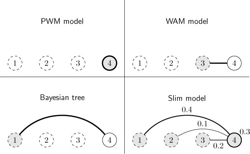
Graphical representation of Slim model. Graphical representation of the dependencies of position 4 (solid node) on other positions (dashed nodes) as modeled by a PWM model, a WAM model, a Bayesian tree and a Slim model. The PWM model assumes independence between position represented by missing edges between nodes and the thick outline of node 4. For a WAM model, the conditional probabilities at position 4 depend on the nucleotides observed at position 3 as indicated by the thick edge, but does not depend on any of the other positions. For a Bayesian tree, the conditional probabilities at position 4 depend on the nucleotides observed at any other position (position 1 in the example). The Slim model is capable of interpolating between all of these cases. In the specific example, the probabilities at position 4 are independent of all other positions with a weight of 0.3 (thick outline of node 4) , while the remaining weight of 0.7 is distributed between preceding positions 1, 2 and 3. These values are chosen for illustration purposes, whereas typically, the weights of the Slim model are less evenly distributed between the different options.

Once dependencies between binding site positions have been learned, an intuitive visualization of these dependencies greatly supports the perception of dependency structures and their biological interpretation. Sequence logos (44) are widely used for visualizing sequence motifs. However, sequence logos are not suited for detecting dependencies between binding site positions, as they assume statistical independence of binding site positions in analogy to PWM models. Hence, extensions of sequence logos have been used, as for instance, sequence logos using adjacent di- and trinucleotides instead of single nucleotides (45). Further attempts have been made to visualize dependencies between binding site positions, which, however, lack the instant perceptibility of the original sequence logo and are largely tied to a specific class of models. Specifically, visualizations for feature motif models (46), hidden Markov models (13) and adjacent dinucleotide models (6) have been proposed.

In this paper, we present dependency logos as a new way of visualizing dependency structures within binding sites. In contrast to sequence logos, dependency logos make dependencies between binding site positions visually perceptible. In contrast to previous approaches, dependency logos are model-free and only require a set of aligned sequences, e.g. predicted binding sites, and, optionally, associated weights as input.

MATERIALS AND METHODS

In this section, we introduce the Slim and LSlim models, explain how we estimate the model parameters, and how we apply the model in practical applications. Subsequently, we introduce dependency logos and give illustrative examples for their advantages compared to sequence logos. Finally, we specify the data that we use in the case studies.

Sparse local inhomogeneous mixture model

We consider DNA sequences where each symbol x_ℓ is from the DNA alphabet Σ = {A, C, G, T}. For modeling dependencies within DNA sequences, we introduce sparse local inhomogeneous mixture (Slim) models that allow for modeling each position within the sequence independently of all other positions or conditionally dependent on some of its predecessor positions.

In the following, we do not explicitly denote the model parameters for the sake of readability. However, each of the P_l(...) terms depends on (some of) the model parameters, and we use the natural parametrization (47,48) for all probabilities. We denote by X_ℓ the random variable for nucleotide x_ℓ, by Y_ℓ the random variable for the conditioning nucleotide, by M_ℓ the hidden random variable for the position of the conditioning nucleotide and by C_ℓ the binary hidden random variable distinguishing between the independent (C_ℓ=0) and conditionally dependent (C_ℓ = 1) cases.

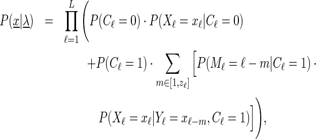
For a (limited) Slim model of distance d, the likelihood of sequence is defined as

(1)

where _ℓ = min (d, ℓ − 1) and the remaining terms have the following meaning:

• P(C_ℓ): The a priori probability that the distribution at position ℓ should be modeled by a weight matrix (C_ℓ = 0, no context dependencies) or by a conditional distribution depending on previous positions (C_ℓ = 1).

• P(X_ℓ|C_ℓ = 0): The unconditional, probability distribution over the nucleotides at position ℓ is similar to a PWM.

• P(M_ℓ|C_ℓ = 1): The a priori probability that position ℓ should depend on position M_ℓ.

• P(X_ℓ|Y_ℓ = x_{ℓ − m}, C_ℓ = 1): The conditional probability distribution over the nucleotides at position ℓ given the nucleotide at position ℓ − m. This (conditional) distribution depends on the nucleotide x_{ℓ − m} but is identical for each of the possible predecessor positions max (ℓ − d, 1), …, ℓ − 1 as indicated by the shared random variable Y_ℓ.

The distance parameter d limits the set of allowed predecessor positions, and, hence, reduces the number of features considered. Conceptually, if d is set to infinity, all predecessor positions (down to position 1) are considered. If d < L − 1, we refer to this model as limited Slim model of distance d (LSlim(d)) and if d = ∞, we refer to this model as full Slim model (Slim) in the following.

In Figure 1, we visualize the dependency structure of a Slim model as defined by its likelihood (Equation (1)) for an exemplary position ℓ = 4. We visualize positions by nodes and possible dependencies by edges. The probability that the position is modeled without context is P(C₄ = 0) = 0.3 depicted close to node 4. In contrast, the probability that the position is modeled with a specific context position is P(C₄ = 1) · P(M₄ = |C₄ = 1) depicted close to the corresponding edges. For instance, the probability that position 4 is modeled with position 2 as context is visualized by the edge between nodes 4 and 2 with P(C₄ = 1) · P(M₄ = 2|C₄ = 1) = 0.1 close to the edge.

Hence, the concept of weighted features is implemented via the distributions P(C_ℓ) and P(M_ℓ|C_ℓ = 1). However, specific choices of these distribution lead to well-known models.

• If for all ℓ P(C_ℓ = 0) = 1, we obtain a PWM model.

• If for all ℓ P(C_ℓ = 1) = 1 and P(M_ℓ = ℓ − 1|C_ℓ = 1) = 1, we obtain a WAM model.

• If for all ℓ P(C_ℓ = 1) = 1 and P(M_ℓ = m_ℓ|C_ℓ = 1) = 1 for one m_ℓ, we obtain a subclass of Bayesian trees, i.e. we obtain a dependency structure that is equivalent to a Bayesian tree. However, in contrast to general Bayesian trees, only the subset of predecessor positions is allowed as ‘parent’ random variable.

In general, we may also obtain all possibilities between those extremes and may partly capture if one position depends on more than one of the other positions.

Encoding feature selection in continuous model parameters in complete analogy to the parameters representing nucleotide probabilities allows for learning both simultaneously using numerical optimization techniques.

Model application

For all applications presented in this paper, models are additionally wrapped in a ‘strand model’, which is a simple mixture model over the two DNA strands such that the enclosed model is applied to an input sequence in both orientations (15).

In case of gcPBM data, we use this strand model in combination with a homogeneous Markov model of order 1 as the background model.

In case of de novo motif discovery using Dimont, this strand model is additionally enclosed in a ZOOPS model (37–39) and a uniform distribution is used as a background model (15).

In the following, we denote the likelihood of the foreground and the background model given the model parameters as and , respectively.

Learning model parameters

We learn model parameters by the discriminative weighted maximum supervised posterior principle (49). To this end, we assign to each input sequence weights _{n, fg} and _{n, bg}, _{n, fg}, _{n, bg} ≥ 0, _{n, fg} + _{n, bg} = 1 representing the probability that this sequence is bound by the transcription factor of interest or not, respectively.

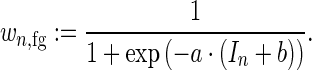
In case of gcPBM data, these weights are based on the PBM intensity I_n for sequence . The foreground weight is determined from a logistic function with parameters a and b as

(2)

The parameters a and b are fitted to the intensities I₁, …, I_N of all input sequences such that the 10th and 90th percentile of the I_n yield _{n, fg} = 0.1 and _{n, fg} = 0.9, respectively.

In case of ChIP-seq data, these weights are based on the ranks of the peak statistics S_n for sequence x_n as described previously (15). Specifically, we compute

(3)

where is the relative rank of the peak statistics of the nth sequence in the data set, r_n is the rank and m = max _n{r_n} is the maximum rank. The parameter q is a user-specified parameter that represents the a priori fraction of sequences that receives a foreground weight >0.5, which is set to the default value of 0.2 for all experiments presented in this paper (15).

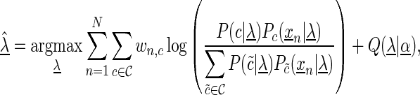
We optimize the model parameters by a weighted variant (15,49) of the discriminative maximum supervised posterior principle (30,50–51)

(4)

where is the set of classes, denotes the a priori probability of class c and denotes the prior on the parameters given hyperparameters . The prior is a transformed product-Dirichlet prior (48) using BDeu hyperparameters (52,24) based on an equivalent sample size of 4. Parameter optimization is performed numerically using conjugate gradients.

Definition of dependency logos

Generating a dependency logo, we start from aligned sequences of length L and, optionally, associated scores, e.g. prediction scores or ChIP peak statistics. We aim at identifying clusters of sequences with co-occurrence of nucleotides at several positions by recursively splitting the data set. Hence given a set of sequences, we compute the mutual information M_{i, j} as a measure of dependence between each pair of positions i and j.

We define D(i) as the average of the three largest mutual information values between position i and any of the remaining positions. Subsequently, we determine that position j yielding the largest D(j) and we determine that position k with the highest mutual information M_{j, k} to the previously selected position j. We then split the set of sequences into 16 partitions according to the nucleotides at positions j and k. To avoid tiny partitions in the visualization, we join all partitions containing <3% of the sequences into the smallest partition containing at least 3% of the sequences. We sort the resulting partitions descendingly according to the average score of the contained sequences if scores are available (as it is the case for all dependency logos presented in this manuscript), or otherwise according to the nucleotide frequencies.

We proceed for each partition recursively until the current set of sequences contains <3% of the initial full set of sequences, D(k) is less than a user-defined threshold, or the maximal recursion depth of 6 is reached.

After partitioning the input sequences in the described manner, we visualize each partition in one row and determine the height of the row relative to the size of the complete data set. We visualize each individual position of a partition by one box and determine the color for this box as the average of the RGB color encodings (A: green, C: blue, G: orange, T: red) of the corresponding nucleotides. In analogy to the scaling of sequence logos, we determine plotting opacity of a box as the relative information content at this position in the partition. Hence, boxes with conserved nucleotides appear in vibrant colors (e.g. positions 8–11 in Figure 2A), whereas less conserved positions become gradually subdued (cf. positions 8, 7 and 6 in Figure 2A).

Figure 2.

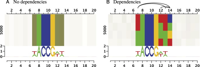
Dependency logos reveal dependencies between binding site positions. While the sequence logos of both data sets are identical, dependency logos reveal dependencies between positions 7, 12, 13 and 14 that are present in data set (B) but not in data set (A).

This procedure allows for distinguishing the dependency structure of the data set visualized in Figure 2A from that of the data set visualized in Figure 2B. While no dependencies exist in data set A and the dependency logo is just one row, we detect several dependencies between positions 7, 12, 13 and 14 in data set B that are visualized by co-occurring colored boxes in several rows. For instance, we observe in Figure 2B that position 13 always shows the same nucleotide (A or T) as position 7, and that position 14 is always C if positions 12 and 13 are T, whereas position 14 is T if position 12 is T and position 13 is A.

To further assist the visual detection of dependencies, we plot a graph structure above the dependency logo, where edges connect all positions exhibiting a significant dependency (chi-squared test, Bonferroni corrected for multiple testing across all combinations of positions) and the darkness of an edge represents the corresponding mutual information value. Finally, we plot a traditional sequence logo below each dependency logo.

For the gcPBM and ChIP-seq analysis, we partition the initial set of sequences into buckets of pre-defined size based on associated scores before starting the recursive partitioning procedure to additionally visualize the variation of dependency structures from top-scoring to low-scoring sites.

Data

gcPBM data

We obtain the gcPBM data of Mordelet et al. (12) (GEO accession number GSE47026) for the human transcription factors Mad2 (also known as Mxi1, 4292 probe sequences), Max (4430 probe sequences) and c-Myc (4917 probe sequences) including the partitioning used for a 10-fold cross validation in the study by Mordelet et al. (12).

ENCODE ChIP-seq data

We obtain from the ENCODE project (21) ChIP-seq data sets for those 63 transcription factors with (i) data sets available for at least two of the ‘Tier 1’ cell types and (ii) uniform peaks available. If multiple such data sets are available for the same cell type but from different labs, we just chose the first uniform peak data set in the list (complete list in Supplementary Text S6.1). For each of the tools tested and each data set, we extract the most suitable sequences in the region of each peak according to the suggestions of the corresponding publications from the hg19 genome sequence obtained from UCSC (http://hgdownload.soe.ucsc.edu/goldenPath/hg19/bigZips/, cf. Supplementary Text S6.3). All data sets comprising the extracted sequences are available from the authors on request.

RESULTS

In this section, we give a brief explanation of dependency logos, which complements the rather formal definition in ‘Materials and Methods’, and, subsequently, we present results of the analysis of gcPBM and ChIP-seq data using Slim and LSlim models.

In a pilot study for these analyses, we test Slim models for classifying artificial sequence data. We find that Slim models are capable of identifying those dependencies between sequence positions that are relevant for classification. On these artificial data, Slim models yield a greater prediction performance than PWM and WAM models, and achieve a prediction performance comparable or slightly better than Bayesian trees using heuristic discriminative structure learning. A detailed presentation of this pilot study is given in Supplementary Text S4.

Introduction to dependency logos

The following presentation of results critically depends on the representation of dependencies and heterogeneities in binding sites by dependency logos. Hence, we give a short introduction to dependency logos in this section, while a formal definition has been given in ‘Materials and Methods’.

Sequence logos (44) are an intuitive method to visualize sequence motifs, but have several disadvantages including the inability to visualize dependencies between positions of binding sites.

To overcome these limitations, we propose dependency logos as an alternative way of representing binding specificities. Dependency logos make dependencies between different motif positions visually perceptible by three key ideas.

First, dependency logos are directly based on binding sites instead of abstract binding motifs, e.g. mononucleotide distributions of PWM models.

Second, we cluster binding sites by their nucleotides at those positions showing the strongest dependencies to other positions. If, for instance, position 14 shows the strongest dependencies to other positions and, of those, the dependency between positions 13 and 14 is the strongest, we create 16 clusters according to the dinucleotide at positions 13 and 14. This procedure may be repeated recursively for each of the clusters (e.g. those sequences with a TC at positions 13 and 14) as detailed in Materials and Methods.

Third, we visualize each cluster as one row of colored boxes using the familiar colors of sequence logos. If more than one nucleotide is present at a certain binding site position in a cluster, we mix the colors representing those nucleotides and set their saturation based on information content in analogy to the height of stacks in sequence logos. We give a step-by-step example for the generation of dependency logos in Supplementary Text S1 and provide an annotated dependency logo in Supplementary Figure S1.

An illustrating example of dependency logos is given in Figure 2. In this case, the sequence logos (lower part) fail to represented dependencies present in data set B. In contrast, the dependencies between positions 7, 12, 13 and 14 are clearly visible as dependency structure and colored boxes in the upper part of the dependency logo of Figure 2B (more details cf. Materials and Methods).

In Supplementary Text S2, we extend the examples above presenting dependency structures that may be present in the data and that can not be distinguished by sequence logos (Supplementary Figure S2). We also use dependency logos in Supplementary Figure S3 to illustrate the rather smooth transition from perceived dependencies to perceived heterogeneities and discuss why both are not clearly separable.

gcPBM data

In a first practical application of Slim and LSlim models, we consider the gcPBM data. Originally, the protocol of gcPBM was introduced by Gordan et al. (20) and uses PBM technology but with probe sequences representing known, aligned binding sites in their genomic context (obtained, e.g. from ChIP experiments) instead of unbiased de-Bruijn sequences representing all k-mers. This technique has the advantage that a greater number of probe sequences are actually bound by the factor of interest and yields a higher-granularity picture of binding specificity and context dependency than universal PBMs. Hence, the gcPBM data sets constitute a near-optimal setting for learning statistical models that are more complex than PWMs like WAM models, Bayesian trees, or the Slim and LSlim models proposed in this paper.

Here, we consider the data of Mordelet et al. (12) for the three human basic helix-loop-helix transcription factors Mad, Max and Myc. All three factors bind to sequences with central palindromic E-box consensus CACGTG. Typically, the consensus positions are referred to as position −3 to +3. This consensus is also present in all probes of the data sets of all three factors and, hence, differences in binding strength between different probes may only result from nucleotides at flanking positions.

In Figure 3, we compare the proposed Slim and LSlim models to a PWM model and to several models that can capture dependencies between binding site positions by means of the squared Pearson correlation coefficient R² as proposed by Mordelet et al. (12) (cf. Supplementary Text S3). As a reference, we include the R² values gained by the regression models of Mordelet et al. (12).

Figure 3.

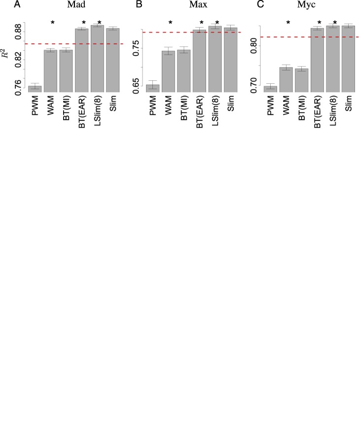
Prediction performance on gcPBM data. Comparison of the prediction performance of the models considered by means of R² in a 10-fold cross-validation experiment. For each of the data sets, (A) Mad, (B) Max, (C) Myc, and each of the models, we plot the mean R² value with the standard error indicated by error bars. Significant differences of one model to the previous one (Wilcoxon signed-rank test, α = 0.05) are indicated by asterisks. As a reference, we plot the R² value achieved by regression models (12) as a dashed line.

We find that the PWM model, which assumes position independence, and the WAM model, which only captures dependencies between adjacent positions, achieve a substantially lower performance than the regression models of Mordelet et al. The Bayesian tree with the structure determined generatively by mutual information between sequence positions (BT(MI)) scores approximately on par with the WAM model. In contrast, the Bayesian tree with the structure determined discriminatively by explaining away residual (53,54) (BT(EAR)) yields R² values that are substantially greater than those achieved by the regression models for the Mad and Myc data sets and slightly better in case of the Max data set. Finally, the performance achieved by the Slim and LSlim models is consistently greater than the performance of the regression models for all three data sets and the performance of the LSLim model is also significantly better (Wilcoxon signed-rank test over the 10 values obtained in the cross validation) than the performance of the Bayesian tree using EAR.

We investigate, which dependencies contribute the most to prediction performance by scrutinizing the dependency structures learned by the different models. We find that for all three data sets, the LSlim model discovers a dependency between positions −4 and +4 directly flanking the central CACGTG consensus, while the remainder of dependencies either involve neighboring positions or are less strong. This dependency is also discovered by the Slim and BT(EAR) models, which also gained large R² values, but is not represented by the PWM, WAM and BT(MI) models performing worse.

Inspecting this dependency in more detail for the Myc data set, we observe that the majority of Myc binding sites follows the consensus CCACGTGG. However, in the less frequent case of an A at position −4, we likely find a T at position +4, while a G at position −4 most likely results in a C at position +4. This dependency structure also becomes perceptible from the dependency logo presented in Supplementary Figure S5A. The dependency structures for Mad and Max are similar, although less pronounced than for Myc, and the differences between nucleotide preferences are rather subtle (Supplementary Figure S5).

Notably, Yang et al. (17) also report Mad and Max to have more similar binding specificities than each of these factors compared with Myc. Evaluating their models employing DNA shape features on the unfiltered gcPBM data set, Yang et al. yield R² values between 0.80 and 0.88. Hence, models utilizing DNA shape features (19) might implicitly contain similar information as appropriate explicit dependency models, e.g. Slim and LSlim.

In summary, we find that Slim and LSlim models improve considerably over models that can only represent dependencies between neighboring binding site positions and that LSlim models score also slightly but significantly better than Bayesian trees using heuristic discriminative structure learning. This improved prediction performance can mostly be attributed to one specific dependency between the positions directly flanking the binding consensus CACGTG. In contrast to Bayesian trees and due to soft feature selection, Slim and LSlim models are also applicable to de novo motif discovery in the Dimont framework (15). We will exploit this fact in the next section, where we test Slim and LSlim models on ChIP-seq data from the ENCODE project.

ChIP-seq data

In a pilot study, we analyze the Dimont (15) framework that we use for applying Slim and LSlim models to ChIP-seq data. Specifically, we test the prediction performance of Dimont using PWM and WAM models compared with MEME (37,55) as a de facto standard, and DiChIPMunk (14) and TFFMs (13) employing first-order dependency models. To this end, we consider ChIP-seq data sets from the ENCODE project (21) for 63 human transcription factors with (i) data sets available for at least two of the ‘Tier 1’ cell types and (ii) peaks from the ENCODE uniform peak calling pipeline (also referred to as ‘uniform peaks’) available. For each transcription factor, we train each of the approaches on the data for one cell type and assess prediction performance on the data for another cell type.

We find that Dimont yields a competitive prediction performance compared to the other approaches. Hence, Dimont may serve as a solid framework for evaluating different dependency models including Slim and LSlim models in the following. We further use this setting for an initial comparison of Slim and LSlim models with PWM and WAM models within the Dimont framework. We find that for the majority of data sets, all of the dependency models (WAM, Slim or LSlim) yield an improved prediction performance compared to the PWM assuming position independence. WAM, Slim and LSlim models each yield the maximum performance for approximately one-third of the data sets, where the exact proportions vary slightly for different performance measures. A detailed presentation of this pilot study is given in Supplementary Text S6.5, Text S6.6 and Supplementary Figures S6–S16.

Comparing models capturing different dependency structures

While overfitting is less likely for the baseline models (PWM and WAM), it might become an issue for the more complex Slim and LSlim models. In addition, in vivo binding measured by ChIP experiments for one transcription factor may—in contrast to in vitro gcPBM data—be affected by competition among different transcription factors with similar binding preference. This, in turn, might induce cell type-specific biases that may skew the measured performance. To approach both problems, we compare the performance of PWM, WAM, Slim and LSlim models in cross-validation experiments in the following.

In Figure 4, we present the results of 10-fold cross-validation experiments on the largest ChIP-seq data set from ENCODE Tier1 for each of the transcription factors considered in the pilot study using wAUC-PR as performance measure. In contrast other performance measures like AUC-ROC, wAUC-PR measures the ability of classifying highly occupied peaks from less occupied ones but also the ability of predicting peak abundances from sequence data. Results for other performance measures (cf. Supplementary Text S3), including AUC-ROC, can be found in Supplementary Figures S17 and S18. We find that the Slim and LSlim models score worse than the PWM model only for a small fraction of data sets, while the WAM model achieves a lower wAUC-PR than the PWM model for a slightly larger fraction of data sets. We also observe that the LSlim model, which captures short-range non-adjacent dependencies, yields the best prediction performance for a greater number of data sets than any of the other models.

Figure 4.

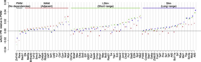
Performance of WAM, LSlim and Slim models relative to a PWM model within the Dimont framework for predictions in a 10-fold cross validation on 63 ENCODE ChIP-seq data sets. For each data set, we plot the performance of WAM, LSlim and Slim models as red, green and blue points, respectively. Here, we use as performance measure the difference of wAUC-PR relative to a PWM model, which is represented by a black line at a value of 0, accordingly. Data sets are grouped according to the model yielding the best performance and, within each group, ordered by the performance of this model. We indicate by a ‘+’: model performs significantly (mean ±2 SD) better than a PWM model; ‘−’: model performs significantly worse than a PWM model; ‘×’: one type of model (LSlim/Slim versus WAM) performs significantly better than the other; ‘*’: combination of ‘+’ and ‘×’.

In total, we find (cf. Supplementary Table S2) that the WAM model yields a significantly (mean ± 2-fold standard error) greater wAUC-PR than the PWM model for 25 of the 63 data sets, while we find the opposite for four data sets. The LSlim model performs significantly better than the PWM for 36 data sets and significantly better than the WAM model for 21 data sets and the opposite is true for one and two data sets, respectively. Finally, the Slim model significantly outperforms the PWM model for 30 and the WAM model for 12 data sets, while we find the opposite for zero and three data sets, respectively.

Considering prediction performance on the level of individual data sets, we find the improvement in prediction performance consistent with the pilot study (E2F4, Nfya, Nfe2, Nfyb, Nrsf, Atf3), whereas for others (Gtf2f1, Fosl1, Brca1) the improvement is less pronounced, which can in part be attributed to the overlaps between cell type-specific data sets. For some data sets (e.g. Rfx5, Sin3a, Stat5), we find that the dependency models yield a greater improvement of prediction performance compared to the PWM model in the cross-validation experiment than it was the case in the pilot study, which might be due to cell type-specific biases (Supplementary Text S6.2).

Interestingly, we consistently find an improvement of prediction performance for Mxi1, which belongs to the Mad protein family, Max and Myc when using dependency models instead of PWMs irrespective of using (in vitro) gcPBM data (Figure 3) or (in vivo) ChIP-seq data (Figure 4).

While this improvement of prediction performance is valuable per se, e.g. if we combine experimental data like DNase I footprints with computational predictions of binding sites, the predictions of Slim and LSlim models can also be used to gain new insights into the binding landscape of transcription factors. To this end, we study dependency logos of predicted binding sites for several transcription factors in the next section.

Dependency structures

We use dependency logos for visualizing the binding sites predicted by different models in ChIP-seq data sets. Compared to standard sequence logos, dependency logos proposed in this paper make dependencies between the different positions of a binding site perceptible.

As a first example, we consider the c-Jun data set (Figure 5), for which the WAM, Slim and LSlim models showed a clear improvement over the PWM model. Accordingly, we find several dependencies between adjacent positions at both flanks of the central consensus TCA in Figure 5A. The dependency structure on the right flank of the consensus does not show a clear pattern and might be related to shape readout (17,18). In contrast, on the left flank, the dependency logo clearly indicates a flexible binding between the two halves of the c-Jun leucine zipper resulting in the dependencies observed. Hence, we may conclude that c-Jun either binds to sequences similar to the consensus TGASTCA or to sequences similar to an elongated consensus TGAYSTCA which can also be represented by two sequence logos (Figure 5B). For Jund (Supplementary Figure S19C), we find a similar pattern. This flexibility has also been found by Badis et al. (1) for Jundm2 in mouse using PBM data and by Mathelier et al. (13) using TFFMs on ChIP-seq data for human Jund. However, the TFFM models required a specific initialization strategy to model this flexibility (13), whereas the Slim model proposed in this paper is capable of learning this flexibility intrinsically. Furthermore, dependency logos allow us to identify this type of dependency structure.

Figure 5.

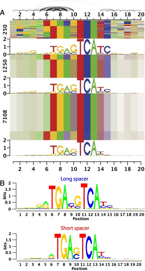
Dependency structure of c-Jun binding sites. For c-Jun, two distinct motifs are captured by the Slim model, which are both composed of the same half sites (TGA and TCA) separated by a varying spacer. These two binding modes are perceptible as distinct blocks in all three blocks in panel (A). In this case, the two binding modes can also be represented by separate sequence logos (B). The bar on the right of panel (A) assigns different blocks of the dependency logo to these sequence logos, where a red bar refers to the short spacer variant and a blue bar refers to the long spacer variant.

As a second example, we consider the Atf3 data set, for which we observed a considerable improvement of prediction performance using Slim and LSlim models in the previous section. We present the dependency logo generated from the predictions of the Slim model for this data set in Figure 6A. We find that the predicted sites are highly heterogeneous following multiple different consensus. A substantial subset of predicted binding sites follows an AP1-like consensus TGACTCA and variations of this motif. However, especially the binding sites with the largest prediction scores depicted in the upmost block of Figure 6A follow a different consensus and show greater variation, including a motif with consensus CSYGGGTTCRANYCCCR without a clearly matching motif in Stamp (56) and a motif with consensus TGACGYA, which is also visible at the bottom of the lowermost block. According to Stamp, the latter partly matches the expected CRE motif. Finally, another subset of predicted binding sites, which is distributed over all three blocks, shows similarities to the E-box consensus CACGTG.

Figure 6.

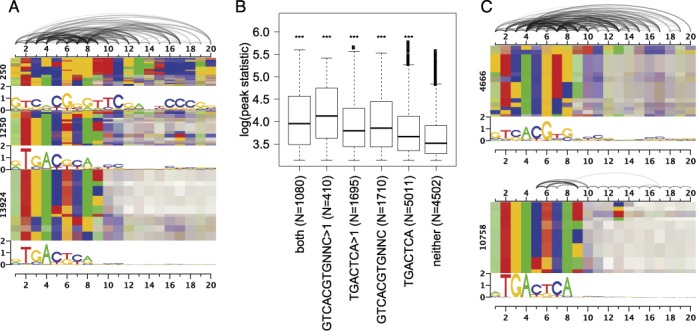
Dependency structure of Atf3 binding sites. For Atf3, broad heterogeneities can be captured by the Slim model. For the binding sites predicted by the Slim model, we plot a dependency logo using all data (A). We learn a two-component mixture model on the predicted binding sites and partition the enclosing sequences under the ChIP peaks according to the occurrence of single and multiple motif instances. For these partitions, we generate box plots of the associated ChIP peak statistics (B). Black asterisks: significant difference to sequences without predicted binding sites (Kolmogorov–Smirnov test, corrected P-values, ***P < 10⁻⁵). We also plot dependency logos for the binding sites assigned to the two components of the mixture model (C).

Previous works (57,58) identified the ATF/CRE consensus as TGACGTCA and the AP-1/TRE consensus as TGACTCA. Several studies (58,59) find that the CRE motif preferred by Atf3 and that most Atf3 ChIP peaks can be explained by direct binding to CRE elements (60), which is in contradiction to our findings. However, other studies also observe cases, where Atf3 binds to the AP-1 motif (61) and not the CRE motif present in the promoters of target genes (62,63). Notably, Kheradpour and Kellis (64) analyze Atf3 ChIP-seq data and find an E-box as the first motif, a motif similar to our CRE-like motif as the second motif and a third motif with consensus CCCG similar to the rightmost part of the high-scoring motif discovered by our approach.

Due to the dichotomous characteristic of predicted sites, we use a two-component PWM mixture model to dissect these two groups (Figure 6C). We find that even after de-mixing, several dependencies between binding site positions persist and both groups are still substantially heterogeneous. Hence, a greater number of mixture components (at least five) would be required to largely represent the different types of binding sites by simple PWM models.

Since we can assign each predicted binding site to a ChIP-seq peak with a given peak statistic, we can—after de-mixing—partition the sequences under the ChIP-seq peaks and their associated peak statistics according to single and multiple occurrences of each of these two motifs or co-occurrences of both motifs (Figure 6B). As expected, all groups with predicted sites yield a significantly higher peak statistic than ChIP-seq regions without predicted sites. We also find that the subset of sequences comprising the CREB-like motif yields higher peak statistics than the AP1-like motif, whereas only 3200 of the 14 408 (22%) peaks can be explained by this motif and 7786 (54%) peaks can be explained by the second, AP1-like motif. Only 1080 of the peaks contain both motifs, which is significantly lower than expected by chance (odds ratio 0.34, P < 10⁻¹⁵⁰, two-sided Fisher's exact test) and indicates that both have the tendency to occur mutually exclusive. It remains unclear whether these observations are due to indirect binding of Atf3 to another transcription factor, for instance other bZIP family members like Fos or Jun (57).

For Nfe2 (Figure 7A), we also observe heterogeneities. However, in this case de-mixing yields two clear motifs without substantial dependencies, where the first is an E-box-like (CACGTG) motif and the second is the expected Nfe2 motif with consensus TGCTGAGTCAY (Supplementary Figure S22A). While the E-box-like motif occurs in only a small subset of predicted sites, the corresponding peak statistics are greater than for the expected motif, especially in case of multiple occurrences of the E-box-like motif (Supplementary Figure S22A). Again, both motifs have a strong tendency to appear mutually exclusive (odds ratio 0.06, P < 10⁻⁹⁰).

Figure 7.

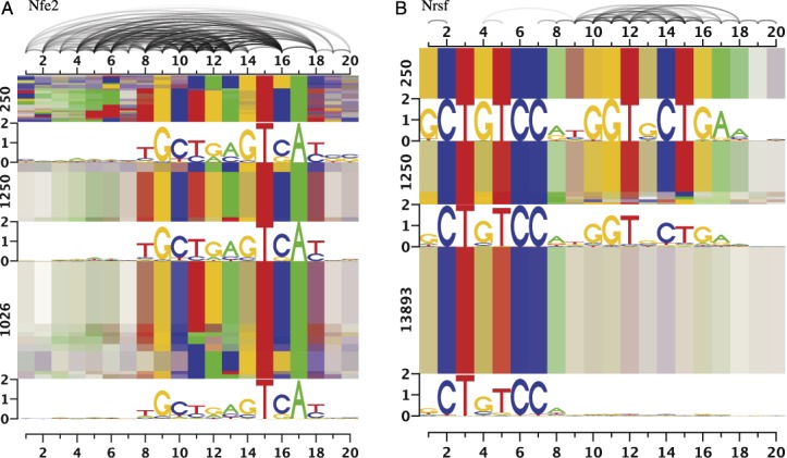
Dependency logos of binding sites predicted by the Slim model for Nfe2 and Nrsf ChIP-seq data sets. For Nfe2, we observe heterogeneities caused by two different, mixed motifs, while we find a partial motif for the majority of Nrsf binding sites.

In case of Nrsf (also known as REST, Figure 7B), we find the canonical Nrsf motif with consensus GCTGTCCNNGGTNCTGA in the sequence under the ChIP-seq peaks with the largest peak statistic (Supplementary Figure S22C). However, the full motif only explains ∼24% of the peaks, whereas the majority of sequences under the ChIP-seq peaks (68%) contain at least the left half site (CTGTCC) of the Nrsf motif. In this case, the dependencies of the Slim model capture the information that the second half of the motif is either completely present (resulting in larger peak statistics) or widely absent (resulting in lower peak statistics). In contrast, a PWM model would only be able to represent a gradual increase of peak statistics with each additional matching base in the second half of the Nrsf motif.

While a dependency of nucleotide conservation on ChIP enrichment of the Nrsf motif has been reported before (65), the clear distinction between two modes of Nrsf binding discovered using the Slim model is novel and might be related to the diverse complexes of Nrsf with other factors (66). For CTCF, which is a transcription factor with a large number of zinc fingers as well (11 versus 8 fingers for Nrsf), a multivalency model has been proposed (67), and a similar binding model might also apply to Nrsf. Finally, several isoforms of Nrsf with differing numbers of zinc fingers have been reported (68), which might also explain the observed binding modes if the antibody used in the experiment has not been specific to one isoform.

In Supplementary Figures S19–S21, we present additional examples of dependency logos of predictions on the ChIP-seq data sets for Jund and Max showing largely adjacent dependencies, Nfyb, E2F4, Taf1 and Tblr1 showing non-adjacent dependencies, Chd2, Mxi1, Rfx5, Sin3a and Stat5 showing heterogeneities, and Elk1 showing negligible dependencies.

It might be tempting to assume that dependency structures could be (more or less) clearly related to transcription factor families. However, we do not find a significant relationship of transcription factor families and the number of neighboring or non-neighboring dependencies, or the degree of heterogeneity (Supplementary Text S6.8, Supplementary Table S3, Supplementary Figure S23).

In summary, we find that Slim and LSlim models may capture dependency structures that range from complex heterogeneities to sparse dependencies between adjacent position or even no substantial dependencies between any motif positions. Each of these situations could also be handled by specialized models, e.g. multi-component mixture models in case of Atf3, spaced PWM models in case of c-Jun or hidden Markov model-like approaches for Nrsf. The main strength of the Slim and LSlim models proposed in this paper is the flexibility to adjust to all these dependency structures without user intervention. Finally, dependency logos allow for dissecting dependencies a posteriori by visual inspection.

DISCUSSION

Building appropriate probabilistic models for transcription factor binding sites is crucial for downstream analyses including genome-wide binding site prediction and identification of target genes. Although statistical dependencies between transcription factor binding site positions have been reported before, they have not been exploited in a fully discriminative manner.

To close this gap, we propose Slim (sparse local inhomogeneous mixture) and LSlim models that use the concept of soft feature selection and, hence, allow for simultaneous feature selection and parameter estimation independent of the learning principle. We demonstrate that Slim and LSlim model in combination with a discriminative learning principle yield an overall improved performance compared to state of the art tools and compared to other probabilistic models on gcPBM and ChIP-seq data. Scrutinizing the results of the individual data sets, we find several cases where a PWM model neglecting dependencies between binding site positions already yields a decent prediction performance. However, for a considerable fraction of data sets, the improvement gained by models capturing dependencies between adjacent and non-adjacent positions is substantial.

Since sequence logos do not allow for visualizing dependencies between binding site positions, we develop dependency logos that allow for visualizing complex dependency structures including neighboring and non-neighboring dependencies, and heterogeneities. Here, we focus on ChIP-seq data sets for those transcription factors with the greatest improvements in prediction performance using Slim or LSlim models. We find that the binding landscapes of the transcription factors considered are highly complex and diverse. For some transcription factors we find secondary or multiple motifs that in general could also be captured by multiple distinct PWM models. For others, however, we find partial motifs, flexible binding modes or dependencies between neighboring and non-neighboring positions, which demand for more complex models.

In a nutshell, there is neither a common dependency structure for all transcription factor binding sites nor dependency structures that can be clearly attributed to transcription factor families. In some cases, PWM models perform sufficiently well, whereas in other cases higher-order dependency models or mixture models improve prediction performance. Hence, modeling transcription factor binding sites profits from flexible motif models that cover a wide range of dependency structures. Slim and LSlim models proposed in this paper are a novel and unbiased approach for capturing all these dependency structures without user intervention.

Dependency logos can also be applied to other aligned sequences including target sites of CRISPR/Cas guideRNAs, microRNA target sites or splice sites for inspecting their dependency structures. However, the applicability of Slim and LSlim models for these types of data has to be proven in further studies.

AVAILABILITY

Slim models and dependency logos are implemented in the open-source Java library Jstacs (69) available at http://www.jstacs.de. At http://galaxy.informatik.uni-halle.de, we provide Galaxy (70) tools for learning Slim models from aligned input sequences, for learning Slim models from ChIP-seq data and for plotting dependency logos. All Galaxy applications are also available for download and can be installed in local Galaxy servers. For learning Slim models from ChIP-seq data, we also provide a multi-threaded command line application at http://www.jstacs.de/index.php/Slim.

SUPPLEMENTARY DATA

Supplementary Data are available at NAR Online.

FUNDING

Institutional budgets.

Conflict of interest statement. None declared.

REFERENCES

- 1.Badis G., Berger M.F., Philippakis A.A., Talukder S., Gehrke A.R., Jaeger S.A., Chan E.T., Metzler G., Vedenko A., Chen X., et al. Diversity and complexity in DNA recognition by transcription factors. Science. 2009;324:1720–1723. doi: 10.1126/science.1162327. [DOI] [PMC free article] [PubMed] [Google Scholar]
- 2.Zhao Y., Stormo G.D. Quantitative analysis demonstrates most transcription factors require only simple models of specificity. Nat. Biotechnol. 2011;29:480–483. doi: 10.1038/nbt.1893. [DOI] [PMC free article] [PubMed] [Google Scholar]
- 3.Morris Q., Bulyk M.L., Hughes T.R. Jury remains out on simple models of transcription factor specificity. Nat. Biotechnol. 2011;29:483–484. doi: 10.1038/nbt.1892. [DOI] [PMC free article] [PubMed] [Google Scholar]
- 4.Benos P.V., Bulyk M.L., Stormo G.D. Additivity in protein–DNA interactions: how good an approximation is it? Nucleic Acids Res. 2002;30:4442–4451. doi: 10.1093/nar/gkf578. [DOI] [PMC free article] [PubMed] [Google Scholar]
- 5.Weirauch M.T., Cote A., Norel R., Annala M., Zhao Y., Riley T.R., Saez-Rodriguez J., Cokelaer T., Vedenko A., Talukder S., et al. Evaluation of methods for modeling transcription factor sequence specificity. Nat. Biotechnol. 2013;31:126–134. doi: 10.1038/nbt.2486. [DOI] [PMC free article] [PubMed] [Google Scholar]
- 6.Jolma A., Yan J., Whitington T., Toivonen J., Nitta K.R., Rastas P., Morgunova E., Enge M., Taipale M., Wei G., et al. DNA-binding specificities of human transcription factors. Cell. 2013;152:327–339. doi: 10.1016/j.cell.2012.12.009. [DOI] [PubMed] [Google Scholar]
- 7.Tomovic A., Oakeley E.J. Position dependencies in transcription factor binding sites. Bioinformatics. 2007;23:933–941. doi: 10.1093/bioinformatics/btm055. [DOI] [PubMed] [Google Scholar]
- 8.Barash Y., Elidan G., Friedman N., Kaplan T. Modelling dependencies in protein-DNA binding sites. In: Vingron M, Istrail S, Pevzner P, Waterman M, editors. RECOMB ′03: Proceedings of the Seventh Annual International Conference on Research in Computational Molecular Biology. NY: ACM Press; 2003. pp. 28–37. [Google Scholar]
- 9.Ben-Gal I., Shani A., Gohr A., Grau J., Arviv S., Shmilovici A., Posch S., Grosse I. Identification of transcription factor binding sites with variable-order Bayesian networks. Bioinformatics. 2005;21:2657–2666. doi: 10.1093/bioinformatics/bti410. [DOI] [PubMed] [Google Scholar]
- 10.Salama R.A., Stekel D.J. Inclusion of neighboring base interdependencies substantially improves genome-wide prokaryotic transcription factor binding site prediction. Nucleic Acids Res. 2010;38:e135. doi: 10.1093/nar/gkq274. [DOI] [PMC free article] [PubMed] [Google Scholar]
- 11.Zhao Y., Ruan S., Pandey M., Stormo G.D. Improved models for transcription factor binding site identification using non-independent interactions. Genetics. 2012;191:781–790. doi: 10.1534/genetics.112.138685. [DOI] [PMC free article] [PubMed] [Google Scholar]
- 12.Mordelet F., Horton J., Hartemink A.J., Engelhardt B.E., Gordân R. Stability selection for regression-based models of transcription factor–DNA binding specificity. Bioinformatics. 2013;29:i117–i125. doi: 10.1093/bioinformatics/btt221. [DOI] [PMC free article] [PubMed] [Google Scholar]
- 13.Mathelier A., Wasserman W.W. The next generation of transcription factor binding site prediction. PLoS Comput. Biol. 2013;9:e1003214. doi: 10.1371/journal.pcbi.1003214. [DOI] [PMC free article] [PubMed] [Google Scholar]
- 14.Kulakovskiy I., Levitsky V., Oshchepkov D., Bryzgalov L., Vorontsov I., Makeev V. From binding motifs in ChIP-seq data to improved models of transcription factor binding sites. J. Bioinform. Comput. Biol. 2013;11:1340004. doi: 10.1142/S0219720013400040. [DOI] [PubMed] [Google Scholar]
- 15.Grau J., Posch S., Grosse I., Keilwagen J. A general approach for discriminative de novo motif discovery from high-throughput data. Nucleic Acids Res. 2013;41:e197. doi: 10.1093/nar/gkt831. [DOI] [PMC free article] [PubMed] [Google Scholar]
- 16.Eggeling R., Gohr A., Keilwagen J., Mohr M., Posch S., Smith A.D., Grosse I. On the value of intra-motif dependencies of human insulator protein CTCF. PLoS One. 2014;9:e85629. doi: 10.1371/journal.pone.0085629. [DOI] [PMC free article] [PubMed] [Google Scholar]
- 17.Yang L., Zhou T., Dror I., Mathelier A., Wasserman W.W., Gordân R., Rohs R. TFBSshape: a motif database for DNA shape features of transcription factor binding sites. Nucleic Acids Res. 2014;42:D148–D155. doi: 10.1093/nar/gkt1087. [DOI] [PMC free article] [PubMed] [Google Scholar]
- 18.Slattery M., Zhou T., Yang L., Dantas Machado A.C., Gordân R., Rohs R. Absence of a simple code: how transcription factors read the genome. Trends Biochem. Sci. 2014;39:381–399. doi: 10.1016/j.tibs.2014.07.002. [DOI] [PMC free article] [PubMed] [Google Scholar]
- 19.Zhou T., Shen N., Yang L., Abe N., Horton J., Mann R.S., Bussemaker H.J., Gordân R., Rohs R. Quantitative modeling of transcription factor binding specificities using DNA shape. Proc. Natl Acad. Sci. U.S.A. 2015;112:4654–4659. doi: 10.1073/pnas.1422023112. [DOI] [PMC free article] [PubMed] [Google Scholar]
- 20.Gordân R., Shen N., Dror I., Zhou T., Horton J., Rohs R., Bulyk M.L. Genomic regions flanking E-box binding sites influence DNA binding specificity of bHLH transcription factors through DNA shape. Cell Rep. 2013;3:1093–1104. doi: 10.1016/j.celrep.2013.03.014. [DOI] [PMC free article] [PubMed] [Google Scholar]
- 21.The ENCODE Project Consortium. An integrated encyclopedia of DNA elements in the human genome. Nature. 2012;489:57–74. doi: 10.1038/nature11247. [DOI] [PMC free article] [PubMed] [Google Scholar]
- 22.Yeo G., Burge C.B. Maximum entropy modeling of short sequence motifs with applications to RNA splicing signals. J. Comput. Biol. 2004;11:377–394. doi: 10.1089/1066527041410418. [DOI] [PubMed] [Google Scholar]
- 23.Posch S., Grau J., Gohr A., Keilwagen J., Grosse I. Probabilistic approaches to transcription factor binding site prediction. In: Ladunga I, editor. Computational Biology of Transcription Factor Binding, Vol. 674 of Methods in Molecular Biology. NY: Humana Press; 2010. pp. 97–119. [DOI] [PubMed] [Google Scholar]
- 24.Heckerman D., Chickering D.M. Learning Bayesian networks: the combination of knowledge and statistical data. Mach. Learn. 1995;20:197–243. [Google Scholar]
- 25.Pietra S.D., Pietra V.D., Lafferty J. Inducing features of random fields. IEEE Trans. Pattern Anal. Mach. Intell. 1997;19:380–393. [Google Scholar]
- 26.Greiner R., Su X., Shen B., Zhou W. Structural extension to logistic regression: discriminative parameter learning of belief net classifiers. 2002. pp. 167–173.
- 27.Ng A., Jordan M. On discriminative vs. generative classifiers: a comparison of logistic regression and naive bayes. In: Dietterich T, Becker S, Ghahramani Z, editors. Advances in Neural Information Processing Systems. Vol. 14. Cambridge, MA: MIT Press; 2002. pp. 605–610. [Google Scholar]
- 28.Yakhnenko O., Silvescu A., Honavar V. Discriminatively trained Markov model for sequence classification. In: Han J, Wah BW, Raghavan V, Wu X, Rastogi R, editors. ICDM ′05: Proceedings of the Fifth IEEE International Conference on Data Mining. Washington, DC: IEEE Computer Society; 2005. pp. 498–505. [Google Scholar]
- 29.Sonnenburg S., Zien A., Ratsch G. ARTS: accurate recognition of transcription starts in human. Bioinformatics. 2006;22:e472–e480. doi: 10.1093/bioinformatics/btl250. [DOI] [PubMed] [Google Scholar]
- 30.Keilwagen J., Grau J., Posch S., Strickert M., Grosse I. Unifying generative and discriminative learning principles. BMC Bioinformatics. 2010;11:98. doi: 10.1186/1471-2105-11-98. [DOI] [PMC free article] [PubMed] [Google Scholar]
- 31.Keilwagen J., Grau J., Paponov I.A., Posch S., Strickert M., Grosse I. De-novo discovery of differentially abundant transcription factor binding sites including their positional preference. PLoS Comput. Biol. 2011;7:e1001070. doi: 10.1371/journal.pcbi.1001070. [DOI] [PMC free article] [PubMed] [Google Scholar]
- 32.Bailey T.L. DREME: motif discovery in transcription factor ChIP-seq data. Bioinformatics. 2011;27:1653–1659. doi: 10.1093/bioinformatics/btr261. [DOI] [PMC free article] [PubMed] [Google Scholar]
- 33.Huggins P., Zhong S., Shiff I., Beckerman R., Laptenko O., Prives C., Schulz M.H., Simon I., Bar-Joseph Z. DECOD: fast and accurate discriminative DNA motif finding. Bioinformatics. 2011;27:2361–2367. doi: 10.1093/bioinformatics/btr412. [DOI] [PMC free article] [PubMed] [Google Scholar]
- 34.Grossman D., Domingos P. Learning Bayesian network classifiers by maximizing conditional likelihood. In: Brodley CE, editor. ICML2004. NY: ACM Press; 2004. pp. 361–368. [Google Scholar]
- 35.Carvalho A.M., Roos T., Oliveira A.L., Myllymäki P. Discriminative learning of Bayesian networks via factorized conditional log-likelihood. JMLR. 2011;12:2181–2210. [Google Scholar]
- 36.Pernkopf F., Bilmes J.A. Efficient heuristics for discriminative structure learning of bayesian network classifiers. JMLR. 2010;11:2323–2360. [Google Scholar]
- 37.Bailey T.L., Elkan C. Fitting a Mixture model by expectation maximization to discover motifs in biopolymers. In: Altman R, Brutlag D, Karp P, Lathrop R, Searls D, editors. Proceedings of the Second International Conference on Intelligent Systems for Molecular Biology. Menlo Park, CA: AAAI Press; 1994. pp. 28–36. [PubMed] [Google Scholar]
- 38.Ao W., Gaudet J., Kent W.J., Muttumu S., Mango S.E. Environmentally induced foregut remodeling by PHA-4/FoxA and DAF-12/NHR. Science. 2004;305:1743–1746. doi: 10.1126/science.1102216. [DOI] [PubMed] [Google Scholar]
- 39.Kim M., Pavlovic V. Technical Report RU-DCS-TR5. NJ: Department of Computer Science, Rutgers University; 2005. Discriminative learning of mixture of Bayesian network classifiers for sequence classification. [Google Scholar]
- 40.Stormo G.D., Schneider T.D., Gold L.M., Ehrenfeucht A. Use of the ‘perceptron’ algorithm to distinguish translational initiation sites. Nucleic Acids Res. 1982;10:2997–3010. doi: 10.1093/nar/10.9.2997. [DOI] [PMC free article] [PubMed] [Google Scholar]
- 41.Staden R. Computer methods to locate signals in nucleic acid sequences. Nucleic Acids Res. 1984;12:505–519. doi: 10.1093/nar/12.1part2.505. [DOI] [PMC free article] [PubMed] [Google Scholar]
- 42.Berg O.G., von Hippel P.H. Selection of DNA binding sites by regulatory proteins: statistical-mechanical theory and application to operators and promoters. J. Mol. Biol. 1987;193:723–743. doi: 10.1016/0022-2836(87)90354-8. [DOI] [PubMed] [Google Scholar]
- 43.Zhang M., Marr T. A weight array method for splicing signal analysis. Comput. Appl. Biosci. 1993;9:499–509. doi: 10.1093/bioinformatics/9.5.499. [DOI] [PubMed] [Google Scholar]
- 44.Schneider T.D., Stephens R.M. Sequence logos: a new way to display consensus sequences. Nucleic Acids Res. 1990;18:6097–6100. doi: 10.1093/nar/18.20.6097. [DOI] [PMC free article] [PubMed] [Google Scholar]
- 45.Eden E., Brunak S. Analysis and recognition of 5’ UTR intron splice sites in human pre-mRNA. Nucleic Acids Res. 2004;32:1131–1142. doi: 10.1093/nar/gkh273. [DOI] [PMC free article] [PubMed] [Google Scholar]
- 46.Sharon E., Lubliner S., Segal E. A feature-based approach to modeling protein-DNA interactions. PLoS Comput. Biol. 2008;4:e1000154. doi: 10.1371/journal.pcbi.1000154. [DOI] [PMC free article] [PubMed] [Google Scholar]
- 47.Klein D., Manning C. Stroudsburg, PA: Association for Computational Linguistics; 2003. Maxent models, conditional estimation, and optimization; p. 8. [Google Scholar]
- 48.Keilwagen J., Grau J., Posch S., Grosse I. Apples and oranges: avoiding different priors in Bayesian DNA sequence analysis. BMC Bioinformatics. 2010;11:149. doi: 10.1186/1471-2105-11-149. [DOI] [PMC free article] [PubMed] [Google Scholar]
- 49.Grau J. Ph.D. Thesis. Martin Luther University Halle–Wittenberg; 2010. Discriminative Bayesian principles for predicting sequence signals of gene regulation. [Google Scholar]
- 50.Roos T., Wettig H., Grunwald P., Myllymaki P., Tirri H. On discriminative bayesian network classifiers and logistic regression. Mach. Learn. 2005;59:267–296. [Google Scholar]
- 51.Cerquides J., de Mántaras R.L. Robust Bayesian linear classifier ensembles. In: Gama J, Camacho R, Brazdil P, Jorge A, Torgo L, editors. Proceedings of the 16th European Conference on Machine Learning. Vol. 3720. Berlin, Heidelberg: Springer; 2005. pp. 72–83. [Google Scholar]
- 52.Buntine W.L. Uncertainty in Artificial Intelligence. San Francisco, CA: Morgan Kaufmann; 1991. Theory refinement of Bayesian networks; pp. 52–62. [Google Scholar]
- 53.Bilmes J.A., Zweig G., Richardson T., Filali K., Livescu K., Xu P., Jackson K., Brandman Y., Sandness E., Holtz E., et al. Department of Electrical Engineering, University of Washington; 2001. Discriminatively structured graphical models for speech recognition. Technical report. [Google Scholar]
- 54.Pernkopf F., Bilmes J.A. De Raedt L, Wrobel S., editors. Discriminative versus generative parameter and structure learning of Bayesian network classifiers. 2005. pp. 657–664.
- 55.Bailey T.L., Williams N., Misleh C., Li W.W. MEME: discovering and analyzing DNA and protein sequence motifs. Nucleic Acids Res. 2006;34:W369–W373. doi: 10.1093/nar/gkl198. [DOI] [PMC free article] [PubMed] [Google Scholar]
- 56.Mahony S., Benos P.V. STAMP: a web tool for exploring DNA-binding motif similarities. Nucleic Acids Res. 2007;35:W253–W258. doi: 10.1093/nar/gkm272. [DOI] [PMC free article] [PubMed] [Google Scholar]
- 57.Hai T., Curran T. Cross-family dimerization of transcription factors Fos/Jun and ATF/CREB alters DNA binding specificity. Proc. Natl Acad. Sci. U.S.A. 1991;88:3720–3724. doi: 10.1073/pnas.88.9.3720. [DOI] [PMC free article] [PubMed] [Google Scholar]
- 58.Gustems M., Woellmer A., Rothbauer U., Eck S.H., Wieland T., Lutter D., Hammerschmidt W. c-Jun/c-Fos heterodimers regulate cellular genes via a newly identified class of methylated DNA sequence motifs. Nucleic Acids Res. 2014;42:3059–3072. doi: 10.1093/nar/gkt1323. [DOI] [PMC free article] [PubMed] [Google Scholar]
- 59.Yin X., DeWille J.W., Hai T. A potential dichotomous role of ATF3, an adaptive-response gene, in cancer development. Oncogene. 2007;27:2118–2127. doi: 10.1038/sj.onc.1210861. [DOI] [PubMed] [Google Scholar]
- 60.Tanaka Y., Nakamura A., Morioka M.S., Inoue S., Tamamori-Adachi M., Yamada K., Taketani K., Kawauchi J., Tanaka-Okamoto M., Miyoshi J., et al. Systems analysis of ATF3 in stress response and cancer reveals opposing effects on pro-apoptotic genes in p53 pathway. PLoS One. 2011;6:e26848. doi: 10.1371/journal.pone.0026848. [DOI] [PMC free article] [PubMed] [Google Scholar]
- 61.Nilsson M., Ford J., Bohm S., Toftgard R. Characterization of a nuclear factor that binds juxtaposed with ATF3/Jun on a composite response element specifically mediating induced transcription in response to an epidermal growth factor/Ras/Raf signaling pathway. Cell Growth Differ. 1997;8:913–920. [PubMed] [Google Scholar]
- 62.Allan A.L., Albanese C., Pestell R.G., LaMarre J. Activating transcription factor 3 induces dna synthesis and expression of cyclin D1 in hepatocytes. J. Biol. Chem. 2001;276:27272–27280. doi: 10.1074/jbc.M103196200. [DOI] [PubMed] [Google Scholar]
- 63.Hagiya K., Yasunaga J.-i., Satou Y., Ohshima K., Matsuoka M. ATF3, an HTLV-1 bZip factor binding protein, promotes proliferation of adult T-cell leukemia cells. Retrovirology. 2011;8:19. doi: 10.1186/1742-4690-8-19. [DOI] [PMC free article] [PubMed] [Google Scholar]
- 64.Kheradpour P., Kellis M. Systematic discovery and characterization of regulatory motifs in ENCODE TF binding experiments. Nucleic Acids Res. 2014;42:2976–2987. doi: 10.1093/nar/gkt1249. [DOI] [PMC free article] [PubMed] [Google Scholar]
- 65.Bruce A.W., López-Contreras A.J., Flicek P., Down T.A., Dhami P., Dillon S.C., Koch C.M., Langford C.F., Dunham I., Andrews R.M., et al. Functional diversity for REST (NRSF) is defined by in vivo binding affinity hierarchies at the DNA sequence level. Genome Res. 2009;19:994–1005. doi: 10.1101/gr.089086.108. [DOI] [PMC free article] [PubMed] [Google Scholar]
- 66.Yu H.-B., Johnson R., Kunarso G., Stanton L.W. Coassembly of REST and its cofactors at sites of gene repression in embryonic stem cells. Genome Res. 2011;21:1284–1293. doi: 10.1101/gr.114488.110. [DOI] [PMC free article] [PubMed] [Google Scholar]
- 67.Nakahashi H., Kwon K.-R.K., Resch W., Vian L., Dose M., Stavreva D., Hakim O., Pruett N., Nelson S., Yamane A., et al. A genome-wide map of CTCF multivalency redefines the CTCF code. Cell Rep. 2013;3:1678–1689. doi: 10.1016/j.celrep.2013.04.024. [DOI] [PMC free article] [PubMed] [Google Scholar]
- 68.Palm K., Belluardo N., Metsis M., Timmusk T.õ. Neuronal expression of zinc finger transcription factor REST/NRSF/XBR gene. J. Neurosci. 1998;18:1280–1296. doi: 10.1523/JNEUROSCI.18-04-01280.1998. [DOI] [PMC free article] [PubMed] [Google Scholar]
- 69.Grau J., Keilwagen J., Gohr A., Haldemann B., Posch S., Grosse I. Jstacs: a java framework for statistical analysis and classification of biological sequences. J. Mach. Learn. Res. 2012;13:1967–1971. [Google Scholar]
- 70.Goecks J., Nekrutenko A., Taylor J., Team T.G. Galaxy: a comprehensive approach for supporting accessible, reproducible, and transparent computational research in the life sciences. Genome Biol. 2010;11:R86. doi: 10.1186/gb-2010-11-8-r86. [DOI] [PMC free article] [PubMed] [Google Scholar]
Associated Data
This section collects any data citations, data availability statements, or supplementary materials included in this article.