Modeling Molecular Kinetics with tICA and the Kernel Trick

Abstract

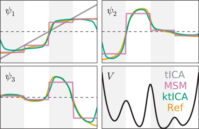
The allure of a molecular dynamics simulation is that, given a sufficiently accurate force field, it can provide an atomic-level view of many interesting phenomena in biology. However, the result of a simulation is a large, high-dimensional time series that is difficult to interpret. Recent work has introduced the time-structure based Independent Components Analysis (tICA) method for analyzing MD, which attempts to find the slowest decorrelating linear functions of the molecular coordinates. This method has been used in conjunction with Markov State Models (MSMs) to provide estimates of the characteristic eigenprocesses contained in a simulation (e.g., protein folding, ligand binding). Here, we extend the tICA method using the kernel trick to arrive at nonlinear solutions. This is a substantial improvement as it allows for kernel-tICA (ktICA) to provide estimates of the characteristic eigenprocesses directly without building an MSM.

1. Introduction

Molecular dynamics (MD) has had a long and important history in computational biology^1,2 and has made many recent contributions toward understanding a variety of biological phenomena, including protein folding,³⁻⁵ protein ligand binding,⁶⁻⁸ and conformational change of large biomolecules.⁹⁻¹³ Though running a large-scale simulation has historically been a demanding task, recent advancements in both software and hardware have made simulations of complex systems possible.¹⁴⁻²⁰ Nonetheless, because of the high-dimensional nature of the resulting time series, the generation of many MD trajectories is not sufficient for providing scientific insight. In fact, data analysis has increasingly become a major barrier in the application of MD simulations.²¹

One analysis technique attempts to estimate the slowly equilibrating collective motions, or eigenprocesses, contained in a simulation (e.g., proteins folding from unfolded conformations, ligands binding to a target, enzymes shifting from an inactive to active state, etc.). These eigenprocesses are useful as they can be measured experimentally, but by constructing them from a simulation, we can provide a level of detail that is unavailable to experiment alone. Markov State Models (MSMs) are one such method that has been useful in a variety of contexts.^{4−6,12,13,22−24} Briefly, an MSM describes continuous dynamics in phase space as a jump process over a finite number of states that partition the space.^25,26 The MSM’s eigenspectrum provides estimates of the eigenprocesses contained in a simulation.

Practically, the construction of an MSM is an active area of research as there are significant hurdles that must be overcome in order to build a model that accurately describes the dynamics contained in a simulation.^26,27 For example, an MSM requires the definition of a state decomposition—that is, a partition of phase space into discrete states. The accuracy of the model relies heavily on the quality of this state decomposition, but although there have been a number of improvements to this process,^22,28−31 there is no consensus on the best method for defining a state space.²⁷

An MSM, however, is merely one way to estimate a system’s eigenprocesses from a simulation. Therefore, we can hope to overcome the practical challenges faced when constructing an MSM by approximating the dynamics within a different scheme. Toward this end, we introduce an extension of time-structure based Independent Components Analysis (tICA) using the kernel trick for estimating the characteristic eigenprocesses contained in a simulation without using an MSM. First, we lay the theoretical foundation for the method, then formulate the problem and derive its solution, and finally, we use the method to analyze several toy models as well as MD simulations of the Fip35 WW domain from Shaw et al.³²

2. Theory

2.1. Transfer Operator Approach

In this section, we briefly discuss Markovian dynamics and the transfer operator approach but leave most details to other works.^25,33 We also note that, for clarity, most of our notation is borrowed from Prinz et al.²⁵

We are interested in discrete-time dynamics in some phase space Ω that are Markovian, ergodic, and time-reversible. Because of these properties, there exists a unique stationary density . This density is properly normalized such that ∫ dx μ(x) = 1. Let x(t) denote a Markov process in Ω. Because of the Markov property, there exists a transition probability density such that p(x,y;τ)dy is the probability of being in some volume (dy) around y after time τ given that the system started at x.

The dynamical progression of the Markov chain can be described via a propagator operator, which maps a probability density at time t, p_t(x), to a new density at time t + τ later, p_t+τ(x):

1

Additionally, there exists a corresponding operator called the transfer operator defined such that

2

The functions u_t(x) are related to probability densities by

3

(While the propagator provides a more intuitive operation, the transfer operator’s eigenfunctions will be the eigenprocesses we actually estimate in the following methods.)

The action of the transfer operator can be decomposed into a series of relaxation processes, which correspond to its eigenfunctions, ψ_i(x), and their eigenvalues, λ_i:

4

where

5

The eigenfunctions of the transfer operator are orthogonal and normalized such that

6

As a result of this decomposition, we can model the dynamics of the Markov chain directly if we have an estimate of the eigenfunctions of the transfer operator. In fact, an MSM provides an estimate of this transfer operator by estimating a finite number of the eigenfunctions as a sum of indicator functions, where the indicator functions define the state decomposition in phase space. However, the MSM is not the only technique that can approximate the transfer operator.

2.2. The Variational Principle of Conformation Dynamics

The eigenvalues of the transfer operator correspond to a relaxation time scale, t_i, which can be measured via the autocorrelation function of a trajectory {x₀,x₁,...,x_t,...} projected onto the corresponding eigenfunction:

7

In recent work from Noé and Nüske,³⁴ it was shown that a variational principle can be derived for the eigenvalues of the transfer operator, meaning that given a mean-centered, integrable function, , the autocorrelation of f at time τ is always less than the autocorrelation of the first nonstationary eigenfunction, ψ₁, of the transfer operator:

8

This is powerful because it implies that one can find the slowest dynamical processes in a simulation without building an explicit estimate of the operator itself, but by directly estimating its eigenfunctions. Nüske et al.³⁵ have successfully constructed estimates of the transfer operator’s top eigenfunctions in the span of a prespecified library of basis functions by leveraging this variational bound. Here, we take a different approach that does not require a predefined basis set.

2.3. Time-Structure Based Independent Component Analysis (tICA)

In what follows, we are working in the space Ω and will assume that it is a Euclidean space with some dimension, d. Therefore, if x and y are in Ω, then x·y = x^Ty denotes the inner product and x ⊗ y = xy^T the outer product between the two length-d column vectors.

Time-structure based Independent Component Analysis (tICA) is an unsupervised learning method for finding projections that decorrelate slowly.^{22,28,36−38} Given a Markov chain in phase space: {x_t ∈ Ω}, tICA attempts to find a vector v ∈ Ω such that the autocorrelation of x_t projected onto v is maximized (eq 9).

9

Here, and τ is some lag time greater than zero. To compute the expectation values in eq 9, assume we can sample M pairs of points in phase space, {(X_t ∈ Ω,Y_t ∈ Ω)}, where X_t is sampled from the equilibrium distribution, μ(·), and Y_t from the transition probability density, p(X_t,· ;τ). Then, we can estimate the time-lag correlation matrix, covariance matrix, and mean vector using a maximum likelihood approach with a multivariate normal approximation (see SI section “Maximum Likelihood Estimator for tICA Matrices”). Let

10

11

where δX_t = X_t–μ, with mean given by

12

Given these matrices, eq 9 becomes

13

It can be shown that the solution to eq 13 is also a solution to the generalized eigenvalue problem:

14

Furthermore, the remaining eigenvectors from eq 14 are the slowest projections constrained to being uncorrelated with the previously found solutions.

This method has proven to be very useful for constructing MSMs that reproduce the slowest time scales in a simulation.^22,28 However, more importantly, since eqs 7 and 9 are the same, the solutions to the tICA problem (tICs) are also solutions to the variational problem and therefore provide estimates of the slowest eigenfunctions of the transfer operator.²⁸ These estimates, however, are crude since the tICs are constrained to be linear functions of the input coordinates, but if we can extend the tICA problem to include nonlinear degrees of freedom then we will be able to estimate the true eigenfunctions more accurately.

2.4. The Kernel Trick

The simplest approach to extending the tICA problem beyond linear combinations of coordinates in Ω is to use a mapping function, Φ:Ω → V, which expands the original representation of the data into a higher-dimensional feature space, V. We can then calculate the linear tICs in the feature space, V, but since Φ is arbitrary, these tICs can in fact be nonlinear functions of the coordinates in Ω. The dimensionality of V, however, could be enormous (or perhaps infinite), and so, this scheme is impractical except in very simple cases. Under certain conditions, however, it is possible to perform analysis in V without ever actually calculating the representations, Φ(x), by employing what is known as the “kernel trick.”

For illustration, we reproduce a simple example from Schölkopf et al.³⁹ of the kernel trick in action. Let and define the mapping function between phase space, , and feature space, V, to be Φ(x) = (x₁², , x₂). Because of this definition, it is easy to show that

15

Equation 15 indicates that we can calculate the dot product in V in one of two ways. We can either compute Φ(x) and Φ(y) and explicitly calculate their dot product or we can simply square the dot product of the vectors in . Either route gives us the same result, but the latter has the advantage of being much easier in cases where the feature space’s dimension is very large—imagine using a polynomial of degree much greater than two in eq 15—or infinite.

Kernels are used commonly in machine learning when extending linear problems to provide nonlinear solutions.³⁹⁻⁴⁴ Any problem that can be rewritten entirely in terms of inner products can be extended to use the kernel trick, and in the following, we show how to rewrite the tICA problem in this way.

2.5. Kernel tICA (ktICA) Solution

Remember that the tICA problem searches for a projection that maximizes the autocorrelation function of a projection onto a vector v. Our goal is to rewrite the optimization problem (eq 13) in terms of only inner products and then apply the kernel trick to solve the tICA problem in high-dimensional feature spaces. First, we assume that the covariance matrix is positive definite. This assumption is only violated when one coordinate can be written as a linear combination of the other coordinates. In these cases, we need only project the data into a nonredundant space and continue the analysis there.

We start with a set of M pairs of points in phase space, {(X_t ∈ Ω, Y_t ∈ Ω)}, where X_t is sampled from the equilibrium distribution, μ(·) and Y_t from the transition probability density, p(X_t,· ;τ). Consider a function Φ:Ω → V that maps points in phase space, Ω, into a higher-dimensional feature space, V. Now we want to solve the tICA problem in this new space V. The solution, v ∈ V, is a solution to the eigenvalue problem given in eq 14. However, the covariance and time-lag correlation matrices are calculated in terms of the vectors in V:

Here, we have used Φ(x) ⊗ Φ(y) to denote the outer product of the two vectors Φ(x), Φ(y) ∈ V. For now, assume that the Φ(X_t) values and Φ(Y_t) values are centered (see Supporting Information (SI) “Centering Data in the Feature Space”).

It can be shown that the solution, v, is in the span of the X_t values and Y_t values, which means that we can write v as a linear combination of the input data points (see SI “tICA Solutions are in the Span of the Input Data”). Let such that

16

We will rewrite the tICA problem in V in terms of a Gram matrix K, where K has 2M rows and 2M columns, defined as

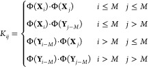17

where Φ(x)·Φ(y) is the inner product between the two vectors Φ(x),Φ(y) ∈ V. In other words, the gram matrix can be broken into four blocks:

18

such that each block is an M × M matrix and

19

20

21

22

Let I_M×M denote the M-dimensional identity matrix and 0_M×M denote an M by M matrix of all zeros. Then, let R be a 2M × 2M matrix given by eq 23.

23

In the SI “Derivation of the ktICA Solution,” we show that the numerator and denominator of the Rayleigh quotient in eq 9 can be rewritten in terms of β and K:

24

25

and so the tICA problem in the feature space V can be written totally in terms of inner products:

26

which is itself a Rayleigh Quotient and so the solutions satisfy the generalized eigenvalue problem:

27

However, solving such problems can be challenging because the matrix KK can have zero eigenvalues, which correspond to directions in V that have zero variance associated with them. These directions are either due to redundant coordinates (in V) or under sampling and so are not desirable solutions to the tICA problem. However, these zero variance directions lead to infinite eigenvalues in eq 27. This issue is not exclusive to the kernel tICA problem and is faced in most kernel learning methods. Several solutions have been reported in the CCA, LDA, and SVM literature that introduce a regularization term.⁴¹⁻⁴³ We use the method applied to kernel-CCA in Mika et al.⁴¹ but realize that another form of regularization may be even more useful. The result is a modified objective function that penalizes the solutions according to the l₂ norm on β.

28

This new Rayleigh Quotient can be written as the solution to a modified generalized eigenvalue problem:

29

For large enough η, the result is a positive definite matrix, KK+ηI_2M×2M, which allows us to compute the solutions reliably. We refer the reader to other kernel methods that use a similar regularization scheme⁴¹⁻⁴³ for a discussion, as well as the Results section Two-Dimensional Brownian Dynamics.

2.6. Connection between ktICA and the Transfer Operator Approach

As in the case of linear tICA, there are many solutions to the ktICA problem (herein called ktICs), where each is the slowest projection subject to being uncorrelated with all of the slower ktICs. Let v⁽ⁱ⁾ ∈ V denote the i^th ktIC and let denote the i^th eigenvector of eq 29 corresponding to v⁽ⁱ⁾:

Because of the variational principle, the ktICs are direct estimates of the transfer operator’s right eigenfunctions:

The first eigenfunction (ψ₀(x) = 1 ∀ x ∈ Ω) is not estimated by ktICA as it is stationary, and so the second eigenfunction is estimated by the first ktIC. However, to directly compare to the eigenfunctions of the transfer operator, we need to ensure that the solutions to the ktICs are normalized correctly.

The eigenfunctions of the transfer operator are orthonormal with respect to the inner product defined in eq 5. Since the first eigenfunction is equal to one for all points x, this means that the eigenfunctions have these properties:

1. All dynamic eigenfunctions (i > 0) have zero mean (). Since the Gram matrix is centered in the feature space (see SI section Centering Data in the Feature Space), the ktICs have zero mean.

2. The eigenfunctions are uncorrelated and are normalized such that they have unit variance (cov(ψ_i(x), ψ_j(x)) = ⟨ψ_i, ψ_j⟩_μ = δ_ij). As shown in the SI section Derivation of the ktICA Solution, the variance of the i^th ktIC, is given by

30

So we can normalize each β⁽ⁱ⁾ such that the variance is one.

Arbitrary points in Ω can be projected onto the ktICs as this operation can be written entirely in terms of inner products:

31

We emphasize here that it is possible to evaluate the value of v⁽ⁱ⁾·Φ(x)—and therefore ψ_i+1(x)—without ever specifying Φ or v⁽ⁱ⁾. In a sense, the ktICs behave like a kernel density estimator, where the value at some point x depends on how close that point is to the training points.

2.7. Model Selection

To solve the ktICA problem, we need to calculate the Gram matrix, K, given in eq 18, which requires the choice of a kernel function that specifies inner products in the feature space. Although there are a variety of kernel functions available, for this work we chose the commonly used Gaussian kernel:

32

Here, x and y correspond to two conformations of a molecule. Technically, these vectors are points in phase space and represent the positions and momenta of all atoms in the simulation. However, in most bimolecular simulations, we do not care to describe the rotation and translation of the molecule. Moreover, because we only have finite sampling, if we attempt to describe rotation and translation in our models, then we will likely do so only by sacrificing accuracy in describing the conformational change that we are interested in. For this reason, for each application we select an internal set of coordinates (e.g., all dihedral angles or contact maps of a protein) to use in eq 32. These coordinates will depend on the particular system being studied, and so we leave their specification to the application sections below.

With the kernel given in eq 32, the gram matrix is defined as

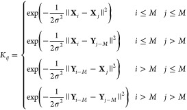33

The solutions to eq 29 provide an explicit form of the estimates of each eigenfunction ψ_i+1:

34

This expression highlights the analogy to a Gaussian kernel density estimator, where we can evaluate ψ_i+1 at any point x based on the eigenvectors from eq 29 and how close x is to each point in the training set.

In addition to the kernel, we must choose the correlation lag time, τ, and the regularization strength, η. In previous studies, tICs were largely unperturbed by the choice of τ;²² hence, for each of our example systems, we fix a τ and ask for the best model given this choice. Therefore, there are two free parameters we must specify before we can solve eq 29: σ and η. Bayes’ theorem demonstrates that the probability of a model given the data is proportional to the probability of the data given the model, which means that we can select a model based on maximizing the model’s likelihood of generating new data. Here, a “model” is the set of ktICs from eq 29 solved with particular values for σ and η. Therefore, our strategy will be to solve eq 29 over a range of values for σ and η and then pick the model that assigns the highest probability to new data.

As the ktICs are estimates of the transfer operator’s eigenfunctions, we can define a likelihood based on eq 4. Let k be a positive integer, then let {(a_t ∈ Ω,b_t ∈ Ω)}_t = 1ⁿ be pairs of test points that were not used in computing the ktICs, where a_t is sampled from the true equilibrium distribution, μ(·), and b_t from the true transition probability density, p(a_t,· ;kτ). Then, the probability of observing all of these transitions can be written in terms of the infinitely many eigenfunctions of the transfer operator:

However, we do not have access to infinitely many eigenfunctions, so we instead truncate the expansion at the top m + 1 eigenfunctions to calculate an approximate probability, P̂.

35

This approximation is better when m is large, or when {λ_i: i > m} are very small. Since the equilibrium probability is not dependent on either of σ and η, we can ignore the μ(·) terms when comparing models. This is especially clear when looking at the approximate log-likelihood:

36

For all applications, we calculate a set of ktICs for a variety of values of σ and η on a subset of the full data set (the training set). Then, eqs 34 and 36 can be used to evaluate the approximate likelihood on {(a_t,b_t)}_t = 1ⁿ – the test set that was initially left out of the calculation. The values of σ and η that are selected are those that are most likely according to eq 36.

One technical issue when calculating these probabilities is that since we truncate the infinite expansion at relatively few ktICs, the resulting probability is not guaranteed to be positive. In practice, this can be difficult to handle but can be avoided by only testing pairs of points that are separated by many multiples of τ. In this way, the faster components we ignore in eq 36 have equilibrated and so the truncated sum is a better approximation of the true (infinite) expansion. Admittedly, this problem likely indicates that defining such a probability based solely on the slowest eigenfunctions of the transfer operator is not possible. There may in fact exist a better scheme for evaluating these models; however, in the results below, we show that, at least for simple systems, the likelihood approach does work.

Computationally, solving the ktICA problem requires finding the solution to eq 29, which is a generalized eigenvalue problem. However, the matrices on either side are 2M × 2M, where M is the number of data points in the training set. This is a computational challenge for all kernel methods, as the solution becomes more difficult to compute as more data is used. Here, we simply limit our analysis to a small portion of the data set. However, there are many sophisticated solutions that have been developed for other kernel-learning methods, and these will certainly be useful in the future.^45,46

3. Results

3.1. One-Dimensional Jump Process

We simulated a Markov jump process on a one-dimensional, four-well potential as suggested in Prinz et al.²⁵ The potential given by

37

was discretized into 100 points between −1 and 1, and a transition matrix was defined such that at each point, there was nonzero probability to move left, move right, or stay at the current point. In each case, the probability to move from point x_i to x_j was proportional to exp[−(V(x_j)–V(x_i))].

We simulated two trajectories of length 10⁶ timesteps. From the first 1000 pairs of transitions separated by 10 time steps were used in the ktICA method. The Euclidean distance between points was used in conjunction with the Gaussian kernel defined in eq 32 to calculate the gram matrix. We used a grid-search approach for determining the best model parameters. The approximate likelihood scores were calculated for 1000 pairs of points sampled from the second trajectory separated by 10 timesteps. In this simple case, there were many models that were roughly the same quality as judged by the likelihood scores (Figure 1).

Figure 1.

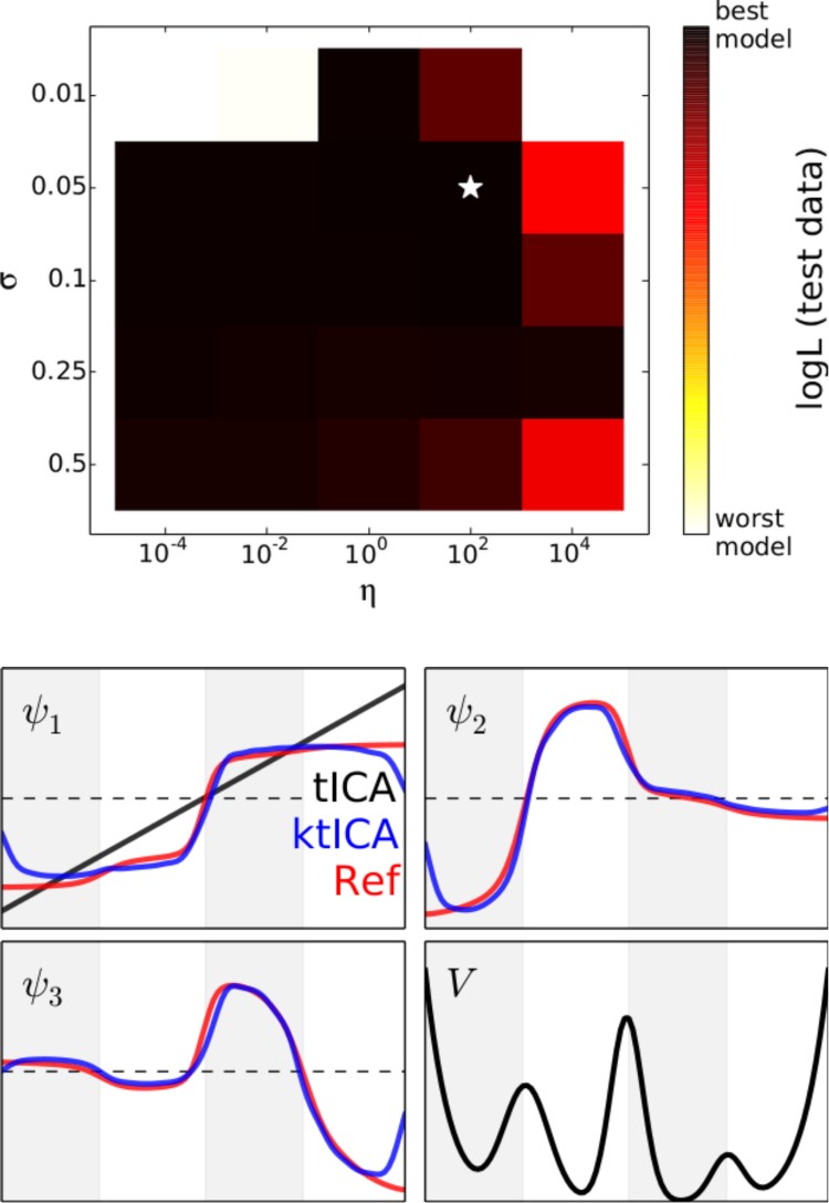
Approximate log likelihood evaluated on test data provided a similar score for most models we tested. Models using a value of 0.01 for σ or a value of 10⁴ for η were given very low scores, while all other models seemed to be good enough. The best model according to the likelihood evaluated on test data correctly determined the top three eigenfunctions for this system. The ktICs are shown in blue while the actual eigenfunctions are shown in red. It is illustrative to remember that the tICA solution is trivial in this one-dimensional case. Even in this simple case, the nonlinearity in the ktICs prove to be essential for estimating the transfer operator’s eigenfunctions.

Since the generating process was itself an MSM, the eigenvalues and eigenvectors are analytically calculable. There are three slow eigenfunctions, corresponding to transitions across the three barriers on this system. The best model correctly determined the slowest three ktICs and are illustrated in Figure 1. These results illustrate the value of nonlinearity in estimating the eigenfunctions of the transfer operator. In fact, since the dynamics take place in a one-dimensional space, there is only one solution to the regular tICA problem, which only (crudely) estimates the slowest eigenfunction of the true transfer operator.

3.2. Two-Dimensional Brownian Dynamics

We also investigated the Müller potential, and simulated dynamics that were governed by

where ζ = 10^–3, kT = 15, and R(t) is a delta-correlated Gaussian process with zero mean, and V(x) was defined as

where a = (−1,–1,–6.5, 0.7); b = (0, 0, 11, 0.6); c = (−10,–10,–6.5, 0.7); A = (−200,–100,–170, 15); X = (1, 0,–0.5,–1); Y = (0, 0.5, 1.5, 1) as suggested by Müller and Brown.⁴⁷ Using the Euler–Maruyama method and a time step of 0.1, we produced two trajectories of length 10⁷ time steps. The initial positions were sampled via a uniform distribution over the box: [−1.5,1.2] × [−0.2,2.0].

The ktICA algorithm was used to analyze the first trajectory by (regularly) sampling 2000 pairs of transitions separated by 10 timesteps. The cross-validation scores were calculated for 1000 pairs of transitions separated by 50 timesteps using the top two ktICs. As there are essentially three local minima in the Müller potential, the top two eigenfunctions should correspond to population transfer between the three wells. The model selected by the likelihood criterion correctly estimates these eigenfunctions (Figure 2) while numerous other models do not.

Figure 2.

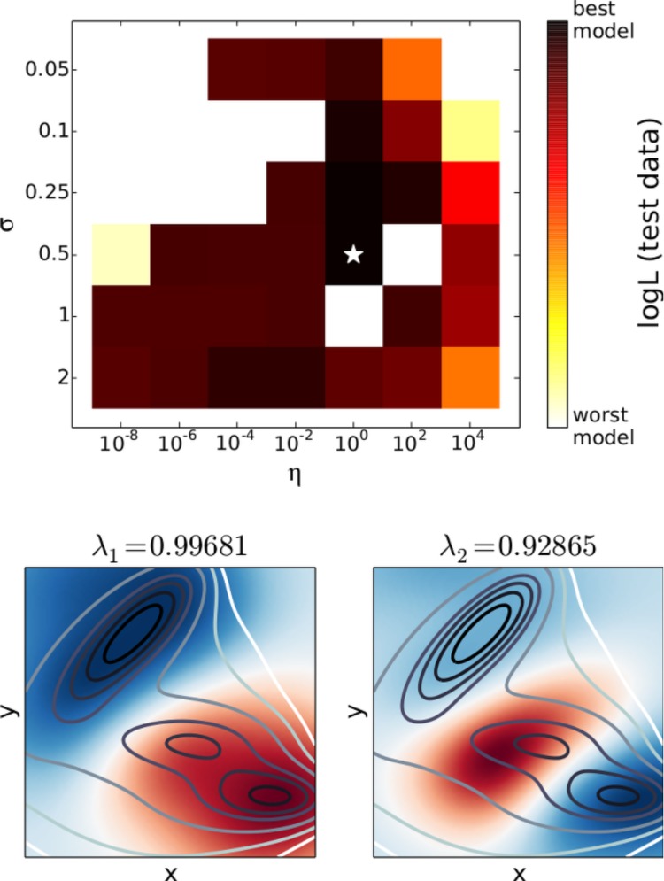
ktICA models for the Müller potential simulations are not as well-behaved as the one-dimensional case. There were a few models that assigned a nonpositive value for the likelihood of test data (white regions above). However, the maximum likelihood model correctly identified the top two eigenfunctions, which separate the three major minima in the potential energy surface. These eigenfunctions are depicted in the bottom two panels, with the red and blue color corresponding to the value of the ktIC. The contour lines denote the potential energy of the system.

The solutions are highly dependent on the choice of the η, which indicates the necessity of regularization. If η is too small, then the ktICs focus on only a few points that are not sampled often in the data set. When it is too large, the eigenvalues are underestimated and the eigenfunctions are distorted from the correct functions. The approximate likelihood evaluated on test data chooses an intermediate value of η whose ktICs correctly separate the three wells in the Müller potential (Figure 3).

Figure 3.

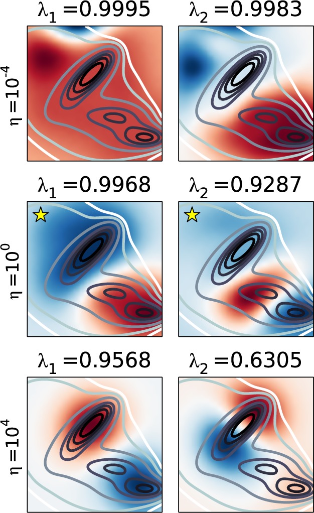
Three models with σ = 0.5 but varying η values are depicted above. These results illustrate the necessity of using regularization. When η is too small (top), the solutions focus on only a few points in the data set that are not sampled heavily, while when it is too large, the solutions are distorted (bottom). Fortunately, the likelihood based model selection criterion picks an intermediate value of η (middle) whose ktICs are better estimates of the actual eigenfunctions.

3.3. Molecular Dynamics of Alanine Dipeptide

A single trajectory of alanine dipeptide (ALA1) was simulated using the amber99sb-ildn force field⁴⁸ in implicit solvent (GBSA) for 500 ns using OpenMM6.0^16,18 with a time step of 2 fs at 300 K using a Langevin integrator. The trajectory was subsampled every 250 fs for analysis and split in half, with the first half serving as the training data and the second serving as the test data. The ktICA calculation was performed by regularly sampling 2000 pairs of points separated by 1.25 ps from the training data. The Gaussian kernel was used in conjunction with a distance metric defined on intra-atomic distances. For each conformation, the distance between all pairs of heavy atoms were computed, which formed a vector of length 45. Then, the distance between two conformations was the Euclidean distance between these vectors.

For the likelihood calculation, we regularly sampled 5000 pairs of points separated by 6.25 ps to ensure that the approximate likelihoods defined by the top two ktICs were non-negative for most models. We should not expect this approximate probability to accurately describe motions at 1.25 ps but would hope that as one looks further in time the probability based on the top two eigenfunctions becomes more accurate. Since alanine dipeptide has been the subject of many computational studies, it is known that the slowest two relaxations occur along the axes of the Ramachandran plot of the two dihedral angles, ϕ and ψ. The most likely model recapitulated these two slow processes (Figure 4).

Figure 4.

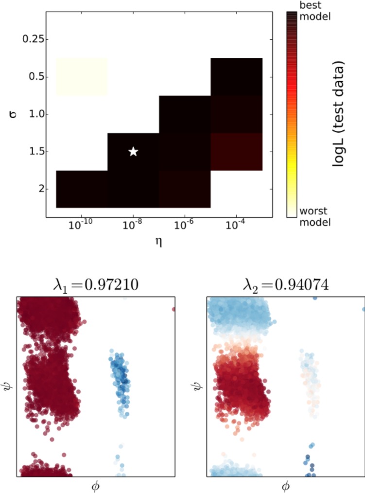
As in the one-dimensional case, there are several models that are very good according to the cross-validation scores, while models with small values of σ and η perform poorly. Alanine dipeptide has been studied extensively, and it is known that the slowest two relaxations occur along the axes of the Ramachandran plot. The projection of the test data set into these axes shows that the top two ktICs correctly identify the slow motions in the alanine dipeptide simulations.

3.4. Molecular Dynamics of Fip35 WW Domain

We reanalyzed the two 100 μs MD trajectories of the Fip35 WW domain performed by Shaw et al.³² The ktICA problem was solved by analyzing 10 000 pairs of transitions separated by 50 ns from the first trajectory. (Note that because of the size of the data set, the pairs of transitions overlapped one another. This is, in a sense, the same as using the sliding window approach for counting transitions when building an MSM, which is common practice.) The Gaussian kernel defined in eq 32 was used with a distance metric defined on the protein’s contact map. Each conformation was represented as a 528-element vector of intramolecular residue–residue distances. Where all pairwise distances were tracked between residues that were at least three amino acids away from each other. The distance between a pair of residues was computed by taking the distance between the two closest heavy atoms in the respective residues. The likelihood defined by the slowest ktIC alone was evaluated on 1000 pairs of transitions separated by 500 ns. This time was long enough to assign non-negative likelihoods to a majority of the models we tested.

The slowest eigenfunctions of the transfer operator for the WW domain are not known, but for the maximum likelihood model, the slowest ktIC is physically reasonable as it separated folded and unfolded states in the simulation (Figure 5). Additionally, the ktIC had a corresponding time scale of 4.4 μs, which is consistent with previous analysis of this data set.^4,27,32

Figure 5.

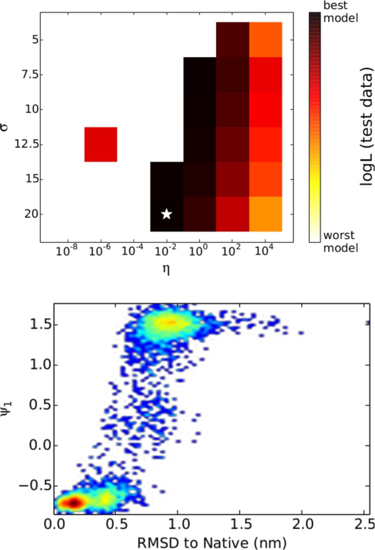
Likelihood defined by only the slowest ktIC was evaluated for the WW domain test data. Again, small values of σ and η produced likelihoods that were often negative for test data; however, there is a region in which all likelihoods were positive. The maximum likelihood model’s slowest ktIC corresponded to the folding transition, as it was correlated with RMSD to the native state. The time scale associated with this ktIC was 4.4 μs, which agrees with previous analysis of this same data set.^4,27,32

4. Conclusions

Though the tICA method has proven to be remarkably successful for building state decompositions for MSM analysis,^22,28,49,50 its solutions are limited because they are constrained to be linear functions of the input coordinates. For this reason, the extension to nonlinear functions by using the kernel trick represents a substantial improvement that allows ktICA to provide estimates of the transfer operator’s eigenfunctions directly, without the use of an MSM. We have shown here that the method can accurately calculate the slowest eigenprocesses of simple systems but admit that there is still work to be done before it can be routinely used for analyzing arbitrarily complex dynamics. Computationally, the matrices in eq 29 scale with the amount of data used, which means that as the systems become larger and more complicated and more data is needed, the eigenvalue problem will become increasingly difficult to solve. However, this problem is not unique to ktICA and, in fact, is ingrained in all kernel learning methods. For this reason, we expect significant improvements to be made rapidly as these methods have been extensively studied in machine learning.

Supporting Information Available

The proof of the maximum likelihood estimators for the tICA matrices as well as the full proof of the ktICA solution can be found in the Supporting Information. This material is available free of charge via the Internet at http://pubs.acs.org/.

The authors declare no competing financial interest.

Funding Statement

National Institutes of Health, United States

References

- Levitt M. Nat. Struct. Mol. Biol. 2001, 8, 392–393. [DOI] [PubMed] [Google Scholar]
- Karplus M.; McCammon J. A. Nat. Struct. Mol. Biol. 2002, 9, 646–652. [DOI] [PubMed] [Google Scholar]
- Lindorff-Larsen K.; Piana S.; Dror R. O.; Shaw D. E. Science 2011, 334, 517–520. [DOI] [PubMed] [Google Scholar]
- Lane T. J.; Bowman G. R.; Beauchamp K.; Voelz V. A.; Pande V. S. J. Am. Chem. Soc. 2011, 133, 18413–18419. [DOI] [PMC free article] [PubMed] [Google Scholar]
- Voelz V. A.; Jäger M.; Yao S.; Chen Y.; Zhu L.; Waldauer S. A.; Bowman G. R.; Friedrichs M.; Bakajin O.; Lapidus L. J.; Weiss S.; Pande V. S. J. Am. Chem. Soc. 2012, 134, 12565–12577. [DOI] [PMC free article] [PubMed] [Google Scholar]
- Buch I.; Giorgino T.; De Fabritiis G. Proc. Natl. Acad. Sci. U.S.A. 2011, 108, 10184–10189. [DOI] [PMC free article] [PubMed] [Google Scholar]
- Shan Y.; Kim E. T.; Eastwood M. P.; Dror R. O.; Seeliger M. A.; Shaw D. E. J. Am. Chem. Soc. 2011, 133, 9181–9183. [DOI] [PMC free article] [PubMed] [Google Scholar]
- Dror R. O.; Pan A. C.; Arlow D. H.; Borhani D. W.; Maragakis P.; Shan Y.; Xu H.; Shaw D. E. Proc. Natl. Acad. Sci. U.S.A. 2011, 108, 13118–13123. [DOI] [PMC free article] [PubMed] [Google Scholar]
- Ivetac A.; McCammon J. A. J. Mol. Biol. 2009, 388, 644–658. [DOI] [PMC free article] [PubMed] [Google Scholar]
- Ostmeyer J.; Chakrapani S.; Pan A. C.; Perozo E.; Roux B. Nature 2013, 121–124. [DOI] [PMC free article] [PubMed] [Google Scholar]
- Lin Y.-L.; Meng Y.; Jiang W.; Roux B. Proc. Natl. Acad. Sci. U.S.A. 2013, 110, 1664–1669. [DOI] [PMC free article] [PubMed] [Google Scholar]
- Shukla D.; Meng Y.; Roux B.; Pande V. S. Nat. Commun. 2014, 5, 3397. [DOI] [PMC free article] [PubMed] [Google Scholar]
- Kohlhoff K. J.; Shukla D.; Lawrenz M.; Bowman G. R.; Konerding D. E.; Belov D.; Altman R. B.; Pande V. S. Nat. Chem. 2014, 6, 15–21. [DOI] [PMC free article] [PubMed] [Google Scholar]
- Shirts M.; Pande V. S. Science 2000, 290, 1903–1904. [DOI] [PubMed] [Google Scholar]
- Shaw D. E.; Deneroff M. M.; Dror R. O.; Kuskin J. S.; Larson R. H.; Salmon J. K.; Young C.; Batson B.; Bowers K. J.; Chao J. C.; Eastwood M. P.; Gagliardo J.; Grossman J. P.; Ho C. R.; Ierardi D. J.; Kolossváry I.; Klepeis J. L.; Layman T.; McLeavey C.; Moraes M. A.; Mueller R.; Priest E. C.; Shan Y.; Spengler J.; Theobald M.; Towles B.; Wang S. C. Commun. ACM 2008, 51, 91–97. [Google Scholar]
- Friedrichs M. S.; Eastman P.; Vaidyanathan V.; Houston M.; Legrand S.; Beberg A. L.; Ensign D. L.; Bruns C. M.; Pande V. S. J. Comput. Chem. 2009, 30, 864–872. [DOI] [PMC free article] [PubMed] [Google Scholar]
- Buch I.; Harvey M. J.; Giorgino T.; Anderson D. P.; De Fabritiis G. J. Chem. Inf. Model. 2010, 50, 397–403. [DOI] [PubMed] [Google Scholar]
- Eastman P.; Friedrichs M. S.; Chodera J. D.; Radmer R. J.; Bruns C. M.; Ku J. P.; Beauchamp K. A.; Lane T. J.; Wang L.-P.; Shukla D.; Tye T.; Houston M.; Stich T.; Klein C.; Shirts M. R.; Pande V. S. J. Chem. Theory Comput. 2013, 9, 461–469. [DOI] [PMC free article] [PubMed] [Google Scholar]
- Götz A. W.; Williamson M. J.; Xu D.; Poole D.; Le Grand S.; Walker R. C. J. Chem. Theory Comput. 2012, 8, 1542–1555. [DOI] [PMC free article] [PubMed] [Google Scholar]
- Pronk S.; Páll S.; Schulz R.; Larsson P.; Bjelkmar P.; Apostolov R.; Shirts M. R.; Smith J. C.; Kasson P. M.; van der Spoel D.; Hess B.; Lindahl E. Bioinformatics 2013, 29, 845–854. [DOI] [PMC free article] [PubMed] [Google Scholar]
- Lane T. J.; Shukla D.; Beauchamp K. A.; Pande V. S. Curr. Opin. Struct. Biol. 2013, 23, 58–65. [DOI] [PMC free article] [PubMed] [Google Scholar]
- Schwantes C. R.; Pande V. S. J. Chem. Theory Comput. 2013, 9, 2000–2009. [DOI] [PMC free article] [PubMed] [Google Scholar]
- Silva D.-A.; Weiss D. R.; Avila F. P.; Da L.-T.; Levitt M.; Wang D.; Huang X. Proc. Natl. Acad. Sci. U.S.A. 2014, 111, 7665–7670. [DOI] [PMC free article] [PubMed] [Google Scholar]
- Bowman G. R.; Geissler P. L. J. Phys. Chem. B 2014, 118, 6417–6423. [DOI] [PMC free article] [PubMed] [Google Scholar]
- Prinz J.-H.; Wu H.; Sarich M.; Keller B.; Senne M.; Held M.; Chodera J. D.; Schütte C.; Noé F. J. Chem. Phys. 2011, 134, 174105. [DOI] [PubMed] [Google Scholar]
- Beauchamp K. A.; Bowman G. R.; Lane T. J.; Maibaum L.; Haque I. S.; Pande V. S. J. Chem. Theory Comput. 2011, 7, 3412–3419. [DOI] [PMC free article] [PubMed] [Google Scholar]
- McGibbon R. T.; Schwantes C. R.; Pande V. S. J. Phys. Chem. B 2014, 118, 6475–6481. [DOI] [PubMed] [Google Scholar]
- Pérez-Hernández G.; Paul F.; Giorgino T.; De Fabritiis G.; Noé F. J. Chem. Phys. 2013, 139, 015102. [DOI] [PubMed] [Google Scholar]
- McGibbon R. T.; Pande V. S. J. Chem. Theory Comput. 2013, 9, 2900–2906. [DOI] [PubMed] [Google Scholar]
- Zhou T.; Caflisch A. J. Chem. Theory Comput. 2012, 8, 2930–2937. [DOI] [PubMed] [Google Scholar]
- Kellogg E. H.; Lange O. F.; Baker D. J. Phys. Chem. B 2012, 116, 11405–11413. [DOI] [PubMed] [Google Scholar]
- Shaw D. E.; Maragakis P.; Lindorff-Larsen K.; Piana S.; Dror R. O.; Eastwood M. P.; Bank J. A.; Jumper J. M.; Salmon J. K.; Shan Y.; Wriggers W. Science 2010, 330, 341–346. [DOI] [PubMed] [Google Scholar]
- Schütte C.; Huisinga W.; Deuflhard P.. Transfer Operator Approach to Conformational Dynamics in Biomolecular Systems; Springer: New York, 2001; pp 191–223. [Google Scholar]
- Noé F.; Nüske F. Multiscale Model. Simul. 2013, 11, 635–655. [Google Scholar]
- Nüske F.; Keller B. G.; Pérez-Hernández G.; Mey A. S.; Noé F. J. Chem. Theory Comput. 2014, 10, 1739–1752. [DOI] [PubMed] [Google Scholar]
- Molgedey L.; Schuster H. Phys. Rev. Lett. 1994, 72, 3634–3637. [DOI] [PubMed] [Google Scholar]
- Blaschke T.; Berkes P.; Wiskott L. Neural Comput. 2006, 18, 2495–2508. [DOI] [PubMed] [Google Scholar]
- Naritomi Y.; Fuchigami S. J. Chem. Phys. 2011, 134, 065101. [DOI] [PubMed] [Google Scholar]
- Schölkopf B.; Smola A.; Müller K.-R. Neural Comput. 1998, 10, 1299–1319. [Google Scholar]
- Schölkopf B.; Smola A.; Müller K.-R. In Artificial Neural Networks—ICANN’97; Gerstner W., Germond A., Hasler M., Nicoud J.-D., Eds.; Lecture Notes in Computer Science; Springer: Berlin, Heidelberg, 1997; Vol. 1327; pp 583–588. [Google Scholar]
- Mika S.; Ratsch G.; Weston J.; Schölkopf B.; Müller K. In Neural Networks for Signal Processing IX, 1999. Proceedings of the 1999 IEEE Signal Processing Society Workshop, Madison, WI, Aug. 23−25, 1999; pp 41−48. [Google Scholar]
- Fukumizu K.; Bach F. R.; Gretton A. J. Mach. Learn. Res. 2007, 8, 361–383. [Google Scholar]
- Bach F. R.; Jordan M. I. J. Mach. Learn. Res. 2003, 3, 1–48. [Google Scholar]
- Cortes C.; Vapnik V. Mach. Learn. 1995, 20, 273–297. [Google Scholar]
- Williams C.; Seeger M. In Proceedings of the 14th Annual Conference on Neural Information Processing Systems, 2001; pp 682−688. [Google Scholar]
- Smola A. J.; Schölkopf B. In Proceedings of the Seventeenth International Conference on Machine Learning (ICML 2000); Morgan Kaufmann: Burlington, MA, 2000; pp 911–918.
- Müller K.; Brown L. D. Theor. Chim. Acta 1979, 53, 75–93. [Google Scholar]
- Lindorff-Larsen K.; Piana S.; Palmo K.; Maragakis P.; Klepeis J. L.; Dror R. O.; Shaw D. E. Proteins Struct. Funct. Bioinf. 2010, 78, 1950–1958. [DOI] [PMC free article] [PubMed] [Google Scholar]
- Lapidus L. J.; Acharya S.; Schwantes C. R.; Wu L.; Shukla D.; King M.; DeCamp S. J.; Pande V. S. Biophys. J. 2014, 107, 947–955. [DOI] [PMC free article] [PubMed] [Google Scholar]
- Razavi A. M.; Wuest W. M.; Voelz V. A. J. Chem. Inf. Model. 2014, 54, 1425–1432. [DOI] [PubMed] [Google Scholar]
Associated Data
This section collects any data citations, data availability statements, or supplementary materials included in this article.