Using Edge Voxel Information to Improve Motion Regression for rs-fMRI Connectivity Studies

Abstract

Recent fMRI studies have outlined the critical impact of in-scanner head motion, particularly on estimates of functional connectivity. Common strategies to reduce the influence of motion include realignment as well as the inclusion of nuisance regressors, such as the 6 realignment parameters, their first derivatives, time-shifted versions of the realignment parameters, and the squared parameters. However, these regressors have limited success at noise reduction. We hypothesized that using nuisance regressors consisting of the principal components (PCs) of edge voxel time series would be better able to capture slice-specific and nonlinear signal changes, thus explaining more variance, improving data quality (i.e., lower DVARS and temporal SNR), and reducing the effect of motion on default-mode network connectivity. Functional MRI data from 22 healthy adult subjects were preprocessed using typical motion regression approaches as well as nuisance regression derived from edge voxel time courses. Results were evaluated in the presence and absence of both global signal regression and motion censoring. Nuisance regressors derived from signal intensity time courses at the edge of the brain significantly improved motion correction compared to using only the realignment parameters and their derivatives. Of the models tested, only the edge voxel regression models were able to eliminate significant differences in default-mode network connectivity between high- and low-motion subjects regardless of the use of global signal regression or censoring.

Introduction

Resting-state functional magnetic resonance imaging (rs-fMRI) can provide an estimate of functional connectivity by computing the correlation of low-frequency (<0.1 Hz) blood-oxygen-level-dependent (BOLD) signal fluctuations in the resting brain between regions of interest (Biswal et al., 1995). Fluctuations during this resting state are thought to represent both spontaneous neuronal activation as well as unconstrained mental activity, such as day dreaming or mind wandering (Fox et al., 2005; Mason et al., 2007). Clinical applications range from presurgical planning to the study of a range of clinical populations and the study of risk factors for psychopathology (Greicius, 2008). While rs-fMRI has been shown to produce reliable and consistent results (Birn et al., 2013; Damoiseaux et al., 2006; Guo et al., 2012; Patriat et al., 2013; Shehzad et al., 2009; Thomason et al., 2011; Van Dijk et al., 2010; Zuo et al., 2010), many aspects of the preprocessing and the processing pipeline remain suboptimal and a consensus standard processing stream is yet to be reached. Among all the methodological challenges with rs-fMRI, subject motion remains one of the most significant.

Head motion has always be known to be an issue in the field of fMRI (Friston, 1996; Jiang, 1995; Oakes et al., 2005; Stillman et al., 1995), but it has recently received even more attention due to the discovery that even very small amounts of shot-to-shot motion or micromovements can significantly distort functional connectivity estimates derived from rs-fMRI data (Christodoulou et al., 2013; Jiang et al., 2013; Jo et al., 2013; Muschelli et al., 2014; Power et al., 2012, 2014, 2015; Satterthwaite et al., 2012, 2013a, 2013b; Van Dijk et al., 2012; Yan et al., 2013a, 2013b). While it is possible to prevent some in-scanner motion through the use of new MRI pulse sequences (Bright and Murphy, 2013; Brown et al., 2010; Kundu et al., 2013; Kuperman et al., 2011; Maclaren et al., 2013; Ooi et al., 2011; White et al., 2010), training on MRI simulators before scanning (Lueken et al., 2012; Raschle et al., 2009), or even the use of head restraints and other bite bars, most data collection either do not or cannot make use of these techniques and motion artifacts are still detectable in these rs-fMRI data.

Different postacquisition methods have been developed to attempt to eliminate the influence of head motion on the final connectivity results. There are two different approaches to minimize motion artifacts: group- and subject-level correction. At the group level, studies have shown that a covariate of no interest (e.g., an estimate of the amount of motion) can be added to the group-level linear regression model to help minimize the influence of head motion on connectivity results (Satterthwaite et al., 2012; Van Dijk et al., 2012; Yan et al., 2013a). While these methods are useful, they are somewhat limited since they assume a linear relationship between the covariate and the motion artifact, which is not necessarily true, and the effect of those methods may only be marginal (Power et al., 2014). The effects of subject motion can also be reduced at the subject level. One approach to reduce the effects of motion is to censor image volumes acquired during periods of high-motion volumes, either removing the data entirely or replacing them with interpolated data (Power et al., 2014). This method, also proposed by another study (Carp, 2013) and which has similarities to AFNI 3dDespike, either introduces synthetic data into the time series or can result in temporal discontinuities, which may bias connectivity results. This censoring can also result in a significant reduction in degrees of freedom. The current study aims at describing and comparing a novel set of subject-level correction methods, both in the presence and absence of censoring.

Current subject-level motion correction methods use two strategies to reduce the influence of subject motion: volume registration (first level) and motion regression (second level). The former consists of realigning each volume acquired in time to one volume from the run or an average volume from the run. The latter method uses the estimated parameters from this realignment as regressors of no interest in a linear regression analysis (Fox et al., 2005; Weissenbacher et al., 2009). More recent strategies have also included the derivative of these motion parameters, yielding 12 nuisance regressors that are currently the most common strategy of second-level motion correction (Power et al., 2012; Van Dijk et al., 2012). Other studies have defined a set 24 motion regressors, consisting of the estimated realignment parameters, the realignment parameters shifted to the prior time point, and these 12 regressors squared, to form a Taylor expansion of motion-related signal changes (Friston, 1996), to further remove the effect of motion from rs-fMRI time series (Power et al., 2014; Satterthwaite et al., 2013b; Yan et al., 2013a). These studies also proposed that, in the future, the aforementioned 24 regressors be used for motion regression instead of the commonly used 12 regressors. Most of the subject-level corrections, to date, use volumetric realignments, which ignore motion occurring within the acquisition of a volume (e.g., motion between slices). More recently, however, a slicewise motion correction method (SLOMOCO) was proposed as a method to correct for head movement occurring between slices (Beall and Lowe, 2014). Furthermore, this study showed that estimated volumetric realignment parameters were often a poor model for motion-related signal changes (Beall and Lowe, 2014).

The goal of this study is to test novel motion regression methods, performed at the subject level, which make use of the information contained at the edges of the brain. The motivation for this approach is that motion artifactually affects the fMRI signal predominantly at the edges of the brain (Jo et al., 2010; Satterthwaite et al., 2013b). Furthermore, motion-induced signal changes are not necessarily linearly related to the six rigid-body realignment parameters. For example, depending on the spatial gradient in signal intensity within the image, motion in one direction may cause a signal increase, but motion in the opposite direction may not necessarily cause a concomitant decrease in signal, thus violating the assumption of linearity with respect to the realignment parameters. In addition, motion may occur only during the acquisition of one slice, and as a result, the signal intensity time course of a particular voxel may not contain all motion events. Our hypothesis is that deriving nuisance regressors from areas most likely to be affected by motion, that is, the edges of the brain, will result in a better model of motion-related signal changes. Such a strategy has been suggested for reducing the effects of task-related motion (e.g., overt speech) on estimates of task-related fMRI activation (Birn, 1999), but has not yet been evaluated for functional connectivity. This data-derived method has the potential to correct for volumetric and between slice motion. We test our models on a publicly and freely available dataset used in previous studies (Jo et al., 2013; Power et al., 2012; Yan et al., 2013a). We also compare our methods to those commonly used by the vast majority of rs-fMRI studies. Finally, we repeat our analysis with and without using global signal regression (GSR) and with and without censoring, as there is currently no consensus on these preprocessing steps. This approach should help rs-fMRI researchers determine the potential benefit of our proposed technique, regardless of the preferred preprocessing pipeline.

Materials and Methods

Participants and image data

For ease of comparison to prior studies, we used the generously donated dataset by Power and colleagues (2012) publicly available on the FCON 1000 project website. We used the same cohort (cohort 1—N=22, 11F, 8.5±1 year) that was used in previous studies (Jo et al., 2013; Power et al., 2012; Yan et al., 2013a). We believe that testing our hypotheses and new methods on a common dataset encourages reproducibility of results as well as comparisons and, therefore, express our gratitude to Power and coauthors for making this dataset available. For more information concerning the acquisition parameters, the subjects, and/or to download the data, please consult the website (http://fcon_1000.projects.nitrc.org/indi/retro/Power2012.html).

fMRI preprocessing

Preprocessing of the rs-fMRI data was implemented using the software AFNI (Cox, 1996) (Fig. 1). The preprocessing steps included the following: removal of the first three volumes of data to get rid of the initial transient in the MR signal; slice-timing correction to correct timing difference due to an interleaved acquisition of slices within a volume; within-run volume registration to reduce the influence of subject motion within the scanner; T1-to-EPI alignment; motion and other nuisance regression (with and without censoring—with and without GSR), spatial blurring (6 mm fwhm), temporal filtering (0.01–0.1 Hz bandpass) all in one step (using 3dTproject); and normalization of EPI data to a common MNI atlas space.

FIG. 1.

Preprocessing and processing pipeline. Green cells indicate single-subject preprocessing and analysis of the rs-fMRI data. Gray cells indicate single-subject processing of the anatomical data. Black cells indicate group-level analysis. Color images available online at www.liebertpub.com/brain

Edge voxel analysis

For each subject, a mask of the brain's edges was generated from the echo-planar image by first generating a brain mask (using AFNI's 3dAutomask) and then subtracting a whole-brain mask to this same mask inflated by two voxels in each direction. Finally, voxels from the resulting edge voxel mask intersecting with the subject's anatomy mask were excluded to ensure that the final edge voxel mask did not include voxel inside the brain incorrectly classified as “edge voxels.” Such voxels include voxels in the ventral portion of the prefrontal cortex, where susceptibility artifacts are common and cause signal dropout. Figure 2 shows an edge voxel brain mask for one representative subject. Edge voxel time courses were extracted from the preprocessed resting data (right after the coregistration step), and the primary features of the temporal signal changes were derived using a temporal principal component analysis (PCA). Twelve principal components (PCs) were derived for each subject. PCA was used to extract relevant features from these time courses since motion-related signal changes are often positive on one edge of the brain and negative at the opposite edge. A simple average of all edge voxel time courses would therefore cancel out the positive and negative signal changes and thus not accurately represent motion-related signal changes. In contrast, PCA generates a set of linear uncorrelated components that reflect the main features of signal variations at the edge of the brain. Such a PCA decomposition approach has previously been used to derive nuisance regressors from CSF and other high variance voxels, primarily to model physiological noise (Behzadi et al., 2007). In this study, we use this idea to specifically derive noise regressors that will best model the signal changes induced by subject motion, and we evaluate the effectiveness of this approach at reducing the influences of subject motion.

FIG. 2.

Edge voxels. Mask of the brain's edge voxels (in red) for a representative subject overlaid on the subject's 3d-rendered anatomical scan and echo-planar images. The mask of edge voxels was derived from the resting-state echo planar image scans. Color images available online at www.liebertpub.com/brain

Motion regression models

In this study, we compare eight different regression models aimed at reducing the correlates of in-scanner motion. In addition, the results will be compared to not doing any motion regression at all. The models are as follows:

• (i) 6mot: 6 parameters of motion coming from the volume registration step of the preprocessing pipeline. This is a common method.

• (ii) 6edge: the first 6 PCs of the edge voxels signal of the preprocessed files.

• (iii) 12mot: same as (i)+the first derivative of those six parameters. This led to regression with 12 parameters of motion. This method is widely used in resting-state functional connectivity processing.

• (iv) 12edge: the first 12 PCs of the edge voxels signal of the preprocessed files.

• (v) 6mot6edge: regressors from (i)+regressors from (ii). This results in a regression with 12 parameters.

• (vi) 6mot6edge*: same as v with the difference that the six PCs of the edge voxels signal were derived after the regression described in (i). This is done to minimize the mutual information contained in the 6 regressors from (i) and (ii).

• (vii) 24mot: 24 motion regressors based on Friston (1996) also examined by other more recent studies (Power et al., 2014; Yan et al., 2013a). The regressors are as follows: same as i, i regressors squared, i regressors at the previous time point, those last 6 regressors squared.

• (viii) 24edge: the first 24 PCs of the edge voxels signal of the preprocessed files.

All of the above regressions were accompanied by the same set of additional nuisance regressors: one averaged white matter and one averaged cerebrospinal fluid time series. GSR is often used as a nuisance regressor and has been shown to have an effect on the motion regression but can also affect the connectivity results (Murphy et al., 2009; Saad et al., 2012); thus, we repeated the above regressions, including GSR. Of note, all of the regressors were detrended and demeaned before the regression analysis.

Censoring

Censoring files were generated using AFNI's 1d_tool.py function, which takes into account motion between two consecutive volumes by calculating the Euclidean norm of the temporal derivative of the motion parameters and then thresholding this metric at a level defined by the user. For the purpose of this study, we chose a threshold of 0.25 mm; this is equivalent to a framewise displacement, or FD, threshold of 0.48 mm (we found that FD values were on average 1.9±0.2 times higher than Euclidean norm values—see Yan et al., 2013a, for a more complete study of the different ways to calculate FD). Figure 3 shows examples of representative one low- and one very high-motion subject. Table 1 shows the amount of time points censored per subject. To study the effect of censoring on the different regression models, we ran our analysis with and without censoring. Data points with high shot to shot motion are ignored in the regression analysis (beta calculation for nuisance regression and connectivity calculation) and are replaced by interpolated values (Power et al., 2014) before temporal filtering. Note that the nuisance regression, censoring, spatial blurring, and temporal filtering occurred all in the same step.

FIG. 3.

Principal components (PCs), motion parameters, and framewise displacement for a representative low-motion subject (left) and very high-motion subject (right). From top to bottom: first six edge PCs, next 6 edge PCs, six edge PCs after doing 6mot regression, 6 parameters of motion, framewise displacement as calculated in the Power paper, framewise displacement as calculated using AFNI. The red line shows the threshold used in this study (0.25 mm). Color images available online at www.liebertpub.com/brain

Table 1.

Number of Time Points Censored Using a 0.25 mm Threshold on Framewise Displacement Metrics Calculated Using AFNI's Euclidean

Subject	# TP censored	Ratio TP censored
1	163	0.37
2	144	0.39
3	54	0.12
4	151	0.34
8	146	0.56
13	17	0.07
16	20	0.08
17	92	0.35
18	8	0.03
19	80	0.31
20	110	0.28
21	39	0.15
24	91	0.35
26	12	0.05
28	4	0.01
49	135	0.35
63	60	0.23
64	23	0.08
65	30	0.10
66	42	0.14
67	12	0.04
68	25	0.10
Mean	66.27	0.21

Metrics

In this study, we compare the different models described above by the means of three different measures: R², DVARS, and temporal signal to noise ratio (tSNR) as defined by Power and colleagues (2012) and also recently used by the same authors (Power et al., 2014).

We first examined the total variance (R²) explained by each model, above and beyond the variance explained by WM and CSF regressors (or the WM, CSF, and Global regressors). To preserve fairness in the comparison between the different models, only models having the same number of regressors are compared to each other. This is because a higher number of regressors are very likely to explain more variance than fewer regressors.

DVARS measures the uniformity of the MR signal intensity within a volume from one time point to the previous (Power et al., 2012). The equation for this measure is as follows:

where I_i (x) represents the signal intensity I at the time point i at the voxel location x, which are then averaged across the entire brain. The lower the number the higher the data quality. This measure has been used by recent studies (Power et al., 2012, 2014; Saad et al., 2012; Satterthwaite et al., 2013a). While it is not known what the whole-brain DVARS should be (as this can also contain neuronal blood oxygenation-level-dependent (BOLD) signal changes to a small extent), comparing the results of different models head-to-head gives us an idea of how they perform relative to one another in reducing motion effects, since the only difference between all the models resides in the regression of the different motion regressors. Note that while lower DVARS may indicate better quality, it does not necessarily mean that the artifact has been completely removed (Power et al., 2014).

Finally, to assess the influence of these noise reduction strategies on the signal at a more basic level, we measured the tSNR (Triantafyllou et al., 2006; Van Dijk et al., 2012).

Statistical testing

Statistical testing was done in MATLAB using an ANOVA followed by Tukey's honest significance difference test for multiple comparison correction.

Functional connectivity processing

In this study, we generated maps of the default-mode network (DMN) using a posterior cingulate/precuneus (PCC) seed for each subject and regression model. The seed used in the present study was a 4-mm-radius sphere located in the posterior cingulate cortex (PCC, MNI coordinates [RAI]: 2, −52, 28). For each regression model, a two-sample t-test was used to observe the differences, within the sample studied here, between high-motion and low-motion subjects. A median split on the ratio of time point censored was used to create a high-motion and a low-motion group; details about how many time points were censored for each subject can be found in Table 1. Since the sample only comprises healthy subjects, there should be no significant differences between the two groups once the artifact is removed. A similar approach has been previously used (Power et al., 2014; Yan et al., 2013a). Finally, we corrected for multiple comparisons using a Monte-Carlo simulation that incorporates the estimated smoothness of the data to determine the smallest number of voxels a cluster needs to include in order for it to have 5% chance to exist by chance or noise only (individual p=0.001, cluster extent=64 voxels).

Results

Principal components

Figure 3 shows the different PCs derived for two representative subjects: one low motion and one high motion. Supplementary Figure S1(Supplementary Data are available online at www.liebertpub.com/brain) shows the spatial distribution of the different PCs over each voxel for a high- and a low-motion subject. None of the observed patterns resembled known networks. Supplementary Figure S2 shows the time series obtained after each motion correction algorithm (in red) compared to the time series before motion regression (in black). The more regressors used, the lower the amplitude of large spikes. The regressors using edge voxel information reduced the amplitude of the spikes compared to the current techniques studied here. Across the entire group of 22 subjects, 73% of the subjects had at least one run for which the first PC was significantly correlated to the global signal (Supplementary Table S1). However, none of the PCs correlated with the derivatives of the six parameters of motion. Furthermore, all of the subjects had at least one run where one or more of the 24 motion parameters (24mot) were correlated with the global signal. Note that the significance threshold used here (cc=0.30 and cc=0.35 for correlation to global signal and the motion parameters, respectively) is very stringent and was determined using the degrees of freedom from the subject for which the lowest amount of time points were acquired (132 time points) and a Bonferroni-corrected p-value of 0.05 based on the number of tests with the most number of runs (6 runs and 6 runs×18 PCs×31 motion parameters+GSR=3348 for correlation to GSR and the motion parameters, respectively).

When the PCs were derived after the 6mot regression was carried out (white PCs in Supplementary Table S2), none of the PCs derived after 6mot was correlated to GSR or the motion parameters (Supplementary Table S2). It is, however, possible that the PCs may be significantly correlated with a linear combination of the motion regressors and derivatives, which is not assessed by the correlation matrix presented here.

Variance explained

Figure 4 and Supplementary Figure S3 show the amount of variance explained by each of the eight models. As expected, the models with 12 regressors explain more variance than the models with only six regressors. This general trend is consistent with results from previous studies (Satterthwaite et al., 2013b). The results were consistent regardless of the use of either GSR or censoring (Table 2).

FIG. 4.

Variance explained (R²) by each of the nuisance regressor sets. For each method, the top bar (green) shows the variance explained by the different motion regression models when censoring was not used; the bottom bar (blue) shows the variance explained by the different motion regression models when not used and was used. Error bars in the graphs represent the standard error of the mean. The results shown here were obtained without the use of global signal regression (GSR). Color images available online at www.liebertpub.com/brain

Table 2.

Results of the Significance Testing for the R², the tSNR, and the DVARS Analysis

For the models with six regressors, 6edge explains significantly more variance than 6mot regardless of GSR and censoring (Table 2). For the models with 12 regressors, regressors incorporating information from edge voxels (12edge, 6mot6edge, 6mot6edge*) explain significantly more variance than the more standard 12mot regressors (Table 2). Comparing the different approaches incorporating edge voxel information, the 6mot6edge* and 6mot6edge methods perform similarly, and 12edge performed significantly better than these two methods (Table 2). These results hold regardless of whether GSR or censoring was performed. Finally, as expected, the 24mot model, with its 24 regressors, explained significantly more variance than the 6 regressor models as well as the 12 regressor models (Fig. 4, Supplementary Fig. S3 and Table 2).

Figure 5 top shows the cumulative variance explained, within the edge voxel masks, by the 12 PCs of edge voxels, 12edge. On average, the first PC accounts for roughly 26% of the variance. Subsequent PCs account for asymptotically decreasing fractions of variance. This fraction of explained variance did not differ much between high-motion and low-motion subjects, with the first PC accounting for 28% of the variance in low-motion subjects and only 24% of the variance in high-motion subjects. The difference in explained variance between the two motion groups increases with increasing numbers of components with the PCs explaining more variance for the high-motion group. Figure 5b shows the fraction of variance explained by the six PCs derived after 6mot regression, as in 6mot6edge* (bottom). The fraction of variance explained by these PCs continues to increase with only gradually diminishing returns. Again, the fraction of explained variance is different for high- and low-motion subjects, where the greater fraction of variance is explained by the PCs in high-motion subjects (Fig. 5).

FIG. 5.

Cumulative variance explained within the edge voxel mask by the 12 principal components (top) and the 6 principal components derived after 6mot regression, as in 6mot6eedge* (bottom) for all subjects (green), high-motion subjects (red), and low-motion subjects (blue). Color images available online at www.liebertpub.com/brain

DVARS

Figure 6 and Supplementary Figure S4 show the DVARS for each correction technique, compared to no correction.

FIG. 6.

DVARS results. For each regressor set, the top bar (green) shows the DVARS for the different motion regression models when censoring was not used; the bottom bar (blue) shows the DVARS for the different motion regression models when censoring was used. Error bars in the graphs represent the standard error of the mean. The results shown here were obtained without the use of GSR. Color images available online at www.liebertpub.com/brain

Regressors incorporating edge voxel information (12edge, 6mot6edge, 6mot6edge*) as well as the 24mot regressor set yield significantly better data quality (lower DVARS) than the standard 12mot whenever censoring is used (Fig. 6, Supplementary Fig. S4 and Table 2). 12edge and 24mot performed similarly and yielded significantly lower DVARS than all the other methods studied. When only six regressors are used, 6edge reduced DVARS more significantly compared to 6mot.

GSR reduces DVARS for all correction methods (Fig. 6 and Supplementary Fig. S4), this difference was found to be statistically significant (p<0.05 corrected). In addition, censoring significantly lowered DVARS.

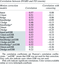
Finally, Table 3 shows the correlation between each subject's average DVARS and their average FD. The motivation for this analysis is that if the motion models removed the motion completely, the correlation between DVARS and FD should be negligible (i.e., DVARS should not be greater for high-motion subjects—those with high FD). When censoring is not used, there is a high correlation between DVARS and FD except for the two 24-regressor models (when GSR is used). However, when censoring is done, the correlation coefficient drops dramatically (e.g., for 6mot it goes from 0.57 to 0.08 when GSR is not used and from 0.63 to 0.22 when it is used). Moreover, censoring made each correlation nonsignificant or anticorrelation (Table 3). Of note, GSR did not affect the correlation except for the two 24-regressor models.

Table 3.

Correlation Between Each Individual Average DVARS Calculated After Regression and Their Average FD

tSNR

Figure 7 and Supplementary Figure S5 show the tSNR results for each of the motion correction methods. Overall, the more regressors used, the higher the tSNR. Similarly to variance explained and DVARS, 6edge yielded better results than 6mot, our 12-regressor models (12edge, 6mot6edge, and 6mot6edge*) performed better than 12mot, and 24edge yielded higher tSNR than 24mot (Fig. 7, Supplementary Fig. S5 and Table 3). Similarly to DVARS, censoring had a positive impact on the results as represented by higher tSNR values (Fig. 7 and Supplementary Fig. S5).

FIG. 7.

tSNR results. For each regressor set, the top bar (green) shows the tSNR for the different motion regression models when censoring was not used; the bottom bar (blue) shows the temporal signal to noise ratio (tSNR) for the different motion regression models when censoring was used. Error bars in the graphs represent the standard error of the mean. The results shown here were obtained without the use of GSR. Color images available online at www.liebertpub.com/brain

Connectivity

Figure 8 shows the differences in DMN connectivity between high- and low-motion subjects for each motion regression model. Only the 24-regressor models were able to significantly diminish or eliminate connectivity differences between the low- and high-motion groups. 24edge was the only model to eliminate connectivity differences between the two groups no matter the use of GSR or censoring. 24mot was only able to do so when GSR was used. When GSR was not used, 24mot was only able to reduce connectivity differences compared to 6- and 12-regressor models but was not able to eliminate those differences (Fig. 8). All the other models resulted in large clusters of high- versus low-motion connectivity differences in the occipital lobe and the lateral temporal cortex, when censoring was not used, while significant clusters located within the DMN, and task-positive networks were visible when censoring was used (Fig. 8). Supplementary Figure S6 shows the group maps for the high- and low-motion groups for each of the motion corrections studied.

FIG. 8.

Default-mode network (DMN) connectivity differences between median-split high- and low-motion subjects for each motion regression model. Left panel shows results when censoring was used, while the right panel shows results when censoring was not used. The green rectangles represent cases where there were no significant differences. The blue clusters show spatial locations where connectivity was either less positive or more anticorrelated in the low-motion group, while warmer colors represent clusters where connectivity was either higher or less anticorrelated in the low-motion group. Note: these results were obtained without the use of GSR. Color images available online at www.liebertpub.com/brain

Discussion

In this study, we set out to test and compare new motion regression models to current standard methods to correct for the effects of in-scanner head motion. We used R², tSNR, DVARS, and functional connectivity (from a PCC seed) as metrics to compare the different methods. The number of regressors to use depends on the available degrees of freedom and desired statistical power. In this study, we chose to examine either 6 or 12 regressors to facilitate comparison with the existing motion regression approaches. Using a higher number of regressors can model a greater amount of variance (with diminishing returns as the number of regressors increase), yet the loss of degrees of freedom should not be underestimated.

Principal components

We have shown in this study that edge voxel regressors explain a lot of the variance due to head motion and are better at removing the effect of motion than current standard techniques. Furthermore, the edge voxel regressors were shown to reduce the amplitude of large spikes (Supplementary Fig. S2). The ideal number of edge voxel regressors will depend on the amount of motion and the number of image volumes acquired. While a significant fraction of variance is explained by the first PC, and the 6 motion realignment parameters, further gains in the variance explained by the PCs rise with only gradually diminishing returns (Fig. 5). PCs, for the 12edge and 6mot6edge models, or the PCs after regressing out the 6 motion parameters, account for greater variance in high-motion subjects since the noise contains a greater contribution from motion. Another interesting finding is the observation that the PCs are not always significantly correlated to the motion parameters. This may be due, in part, to the greater sensitivity of the PCs to slicewise motion not accurately captured by volumetric realignment (Beall and Lowe, 2014).

While the first PC of the edge voxel time series was often correlated with the global signal, it should be kept in mind that the global signal can contain significant amounts of motion-related signal change, as motion-related signal changes occur throughout the brain (Power et al., 2014, 2015; Satterthwaite et al., 2013b; Yan et al., 2013a, 2013b). Furthermore, one or more of the 24 motion realignment parameters (24mot) also correlated significantly with the global signal, further supporting the possibility that aspects of the motion are captured in the global signal. Finally, recent studies have also shown that even pure noise regressors can account for neuronal activation-like patterns across the brain (Bright and Murphy, 2015). The reason for this is that, unless the noise is perfectly orthogonal to the signal of interest, the fit of that noise regressor is similar in areas that have highly correlated (i.e functionally connected) fluctuations. The removal of signals of interest, at least to a certain degree, is therefore always a possibility, even with pure noise regressors, but this likelihood increases with a large number of nuisance regressors. Care should therefore be taken to minimize the number of nuisance regressors.

6-regressor models

We studied two 6-regressor models: 6mot and 6edge. 6edge regressors explain significantly greater amount of variance compared to the 6mot regressors. DVARS were found to be significant decreased when 6edge was used. Finally, tSNR was significantly increased when 6edge was used. All in all, the 6edge model outperformed the current standard for 6-regressor models. However, none of these models was able eliminate DMN connectivity differences between the high- and low-motion groups, thus indicating that improvements are necessary to completely get rid of motion artifacts; adding more regressors might be beneficial. The conclusions stand regardless of the use of GSR or censoring.

12-regressor models

We studied four 12-regressor models: the standard 12mot and our own models 12edge, 6mot6edge, and 6mot6edge*. The models based on edge voxels explained significantly more variance than the current standard 12mot. In addition, the first 12 PCs from the edge voxel time series (12edge) performed better than a simple combination of the 6 realignment parameters with the first 6 PCs of the edge voxels before any regression (6mot6edge) and the combination of the 6 realignment parameters with the first 6 PCs of edge voxels after regression of these realignment parameters (6mot6edge*). Once again, our 12-regressor models incorporating edge voxel information had significantly lower DVARS than the standard 12mot. 12edge was the 12-regressor correction method that yielded significantly lower DVARS. Finally, 12edge yielded significantly higher tSNR than all the other 12-regressor models studied here. All in all, the 12edge model outperformed the current standard for 12-regressor models. However, none of the four models was able to eliminate DMN connectivity differences between the high- and low-motion groups, thus indicating that improvements are necessary to completely get rid of motion artifacts; adding more regressors might be beneficial. The conclusions stand regardless of the use of GSR or censoring.

24-regressor models

We studied two 24-regressor models: 24mot, derived using the motion parameters, and our own model 24edge. The model based on edge voxels explained significantly more variance than the current standard 24mot. Once again, our 24-regressor models incorporating edge voxel information had significantly lower DVARS than the standard 24mot. Also, 24edge yielded significantly higher tSNR values. Finally, 24edge was the only model to eliminate DMN connectivity differences between the low- and high-motion subjects. 24mot was only able to do so when GSR was used. All in all, the 24edge model outperformed the 24-regressor model proposed previously to replace 12mot (Friston, 1996; Power et al., 2014; Satterthwaite et al., 2013b; Yan et al., 2013a). The conclusions stand regardless of the use of GSR or censoring.

12- versus 6-regressor models

As expected, the 12-regressor models outperformed the 6-regressor models in terms of variance explained and data quality; the six added regressors in our 12edge model accounted for roughly 45% more variance than the 6edge model (Fig. 4). This is not surprising, as adding more regressors take more variance into account. For DVARS, a similar pattern emerges likely due to added noise removal coming from the added information contained in the additional regressors. The 12-regressor models increased tSNR values significantly. Models with a higher number of regressors have also been shown to reduce the number of significantly different connections between high- and low-motion groups, as well as a lower correlation between subject motion and pairwise connectivity (Satterthwaite et al., 2013b). In summary, our results show a clear advantage of using 12-regressor models over the 6-regressor models for motion correction.

12- versus 24-regressor models

The 24-regressor models were found to explain more amount of variance and yield data of higher quality (as measured by DVARS and tSNR) than the best 12-regressor models (12edge *). Moreover, only the 24-regressor models were able to reduce (e.g., 24mot) or completely eliminate (e.g., 24edge) the DMN connectivity differences between the high- and low-motion groups. In summary, our results show a clear advantage of using the 24-regressor over the 12-regressor models for motion correction.

The effect of censoring

Significant fractions of variance were explained by the edge voxel regressors even after motion censoring. This demonstrates that our edge voxel models represent motion beyond merely large motion spikes, for example, by including slower drifts. If only large motion spikes were represented by our models, our models would explain very little to no additional variance when censoring is used. Censoring significantly reduced the DVARS for all methods. The reduction in DVARS with censoring is not surprising, since the primary difference in signal between successive images occurs when there is motion. Censoring these time points reduces the difference. Similarly, censoring was associated with increased tSNR. This increase in tSNR is also not surprising since the removal of motion-related spikes decreases standard deviation.

The effect of using GSR

According to Figure 4 and Supplementary Figure S3, GSR appears to not impact the fraction of variance explained. This was further demonstrated in Table 3 since the correlation coefficients between DVARS and FD were very similar with and without GSR (except for 24edge and 24mot). However, as seen in Figures 6, 7, and Supplementary Figures S4, S5, GSR significantly reduced DVARS and increased tSNR. This indicates that GSR positively impacts data quality. However, studies have also shown that GSR can introduce anticorrelations (Murphy et al., 2009) and alter group differences in functional connectivity (Gotts et al., 2013; Saad et al., 2012, 2013). These are significant problems, and therefore, we cannot recommend the use of GSR.

A further potential model would be to combine edge voxel PCs with the 24mot method. However, the correlation between the PCs and a subset of the 24mot regressors shows that using this combination would result in an unnecessary redundancy and a reduced effectiveness compared to the lost degrees of freedom (Supplementary Table S2). Another possibility would be to first do the 24mot regression and then derive the PCs in a similar manner as the 6mot6edge* set of regressors). However, the effects of such a large loss in degrees of freedom should be carefully considered and not be underestimated. BOLD sensitivity can be decreased by increasing the number of regressors and increasing the complexity of the regression model (Beall, 2010; Beall and Lowe, 2014).

Other data driven models

PCA has previously been used in the context of denoising rs-fMRI data using the correction method CompCor (Behzadi et al., 2007). This method creates regressors using PCA on a noise mask consisting in voxels having the highest standard deviation voxels, which are usually made of white matter, cerebrospinal fluid, vessels, and brain edge regions. Given the nature of these regions, it is possible that the resulting PCs represent mostly physiological processes. In the current study, we focused on the edge voxels to create a set of regressors more specific to motion than those proposed in CompCor.

Recently, another denoising method called FIX has been proposed (Griffanti et al., 2014; Salimi-Khorshidi et al., 2014). This powerful method uses independent component analysis (ICA) on preprocessed data (rigid-body registration, spatial and temporal smoothing) to extract a large set of components that are then automatically classified as being artifactual (physiological noise, motion, or unknown origin) or signal of interest. To identify the motion-related components, they are compared to five different edge masks (different thicknesses). Contrary to our mask, which includes voxels outside of the brain but having at least a face in common with the brain, the masks from FIX include voxels that are inside of the brain. Given this difference and the fact that a temporal-PCA and a spatial-ICA are quite different operations, we obtain different components generated by FIX. One potential drawback of FIX method is the number of components used to denoise the data. The most recent implementations of FIX remove 60 artifactual components, and thus, degrees of freedom. This correction, when combined with an additional 24 nuisance regressors from the 24mot model, can result in an unacceptable loss of degrees of freedom for many studies.

Limitations

While it is beneficial to use a commonly utilized dataset and while the sample provided us with statistically significant results, a larger sample may shed more light on the effect of GSR on motion correction as well some potential tSNR differences. A larger sample would also be beneficial to validate the connectivity differences between high- and low-motion subjects. Also, due to the lack of physiological data, it was not possible for us to test the efficiency of our models associated with nuisance regressors other than WM and CSF, such as RETROICOR (Glover et al., 2000), RVTCor (Birn et al., 2006), and RVHRCor (Chang and Glover, 2009). A potential concern when deriving nuisance regressors from the data itself is the possibility of removing true neuronal activity-related BOLD signal fluctuations or signal of interest. However, we believe this to be unlikely for our proposed method. As shown in Figure 2, the edges used to define motion-related signal changes do not extend into the brain (e.g., they do not follow sulci or include regions such as the vmPFC). Motion-induced signal changes at these edges tend to be much larger than typical BOLD responses. In addition, voxels at the edge of the brain that contain true BOLD activation are likely to be much fewer in number than voxels containing motion-related signal changes. It is thus unlikely that neuronal BOLD signal changes would contribute a significant amount of variance to the edge voxel time series. Moreover, the fit of each PC with each voxel of the brain was visually inspected for a high- and a low-motion subject. None of the PCs exhibited known network connectivity patterns.

Conclusion

In this study, we set out to compare and contrast current commonly used models of motion regression to novel motion regression models making use of the information contained in the EPI's voxels located at the edge of the brain. We found that using regressors containing information from the brain's edge voxels led to better motion regression and better data quality. We found that if a study has sufficiently high degrees of freedom such that the inclusion of a large number of additional regressors is not a significant concern, using a 24-regressor model such as our 24edge model significantly improves the data. We also found that, within the scope of the study, only the 24edge model was found to eliminate DMN connectivity differences between low- and high-motion subjects. If degrees of freedom are an issue (e.g., due to short scan time or heavy censoring), the use of the 12edge model would be an appropriate choice for motion correction. Our results also point out that the use of censoring in conjunction with 24edge is recommended. The use of GSR further reduces noise, but raises significant concerns due to potential alterations to the within-subject and between-subject covariance structure.

Acknowledgments

This work was funded by the NIH grant RC1MH090912, R21MH101526, P50MH100031, the Wisconsin Alumni Research Foundation, and the HealthEmotions Research Institute. The authors do not report any conflicts of interest. The authors wish to thank J.D. Power and the Washington University group for making their dataset available to the public.

Author Disclosure Statement

The authors have nothing to disclose.

References

- Beall EB. 2010. Adaptive cyclic physiologic noise modeling and correction in functional MRI. J Neurosci Methods 187:216–228 [DOI] [PubMed] [Google Scholar]
- Beall EB, Lowe MJ. 2014. SimPACE: generating simulated motion corrupted BOLD data with synthetic-navigated acquisition for the development and evaluation of SLOMOCO: a new, highly effective slicewise motion correction. Neuroimage 101C:21–34 [DOI] [PMC free article] [PubMed] [Google Scholar]
- Behzadi Y, Restom K, Liau J, Liu TT. 2007. A component based noise correction method (CompCor) for BOLD and perfusion based fMRI. Neuroimage 37:90–101 [DOI] [PMC free article] [PubMed] [Google Scholar]
- Birn RM.Functional Resonance Imaging in the Presence of Task-Induced Motion, Biophysics Research Program, Medical College of Wisconsin 1999.
- Birn RM, et al. . 2006. Separating respiratory-variation-related fluctuations from neuronal-activity-related fluctuations in fMRI. Neuroimage 31:1536–1548 [DOI] [PubMed] [Google Scholar]
- Birn RM, et al. . 2013. The effect of scan length on the reliability of resting-state fMRI connectivity estimates. Neuroimage 83:550–558 [DOI] [PMC free article] [PubMed] [Google Scholar]
- Biswal B, et al. . 1995. Functional connectivity in the motor cortex of resting human brain using echo-planar MRI. Magn Reson Med 34:537–541 [DOI] [PubMed] [Google Scholar]
- Bright MG, Murphy K. 2013. Removing motion and physiological artifacts from intrinsic BOLD fluctuations using short echo data. Neuroimage 64:526–537 [DOI] [PMC free article] [PubMed] [Google Scholar]
- Bright MG, Murphy K. 2015. Is fMRI “noise” really noise? Resting state nuisance regressors remove variance with network structure. Neuroimage 114:158–169 [DOI] [PMC free article] [PubMed] [Google Scholar]
- Brown TT, et al. . 2010. Prospective motion correction of high-resolution magnetic resonance imaging data in children. Neuroimage 53:139–145 [DOI] [PMC free article] [PubMed] [Google Scholar]
- Carp J. 2013. Optimizing the order of operations for movement scrubbing: comment on Power et al. Neuroimage 76:436–438 [DOI] [PubMed] [Google Scholar]
- Chang C, Glover GH. 2009. Effects of model-based physiological noise correction on default mode network anti-correlations and correlations. Neuroimage 47:1448–1459 [DOI] [PMC free article] [PubMed] [Google Scholar]
- Christodoulou AG, et al. . 2013. A quality control method for detecting and suppressing uncorrected residual motion in fMRI studies. Magn Reson Imaging 31:707–717 [DOI] [PMC free article] [PubMed] [Google Scholar]
- Cox RW. 1996. AFNI: software for analysis and visualization of functional magnetic resonance neuroimages. Comp Biomed Res 29:162–173 [DOI] [PubMed] [Google Scholar]
- Damoiseaux JS, et al. . 2006. Consistent resting-state networks across healthy subjects. Proc Natl Acad Sci U S A 103:13848–13853 [DOI] [PMC free article] [PubMed] [Google Scholar]
- Fox MD, et al. . 2005. The human brain is intrinsically organized into dynamic, anticorrelated functional networks. Proc Natl Acad Sci U S A 102:9673–9678 [DOI] [PMC free article] [PubMed] [Google Scholar]
- Friston KJ. 1996. Movement-related effects in fMRI time-series. Reson Med 35:346–355 [DOI] [PubMed] [Google Scholar]
- Glover GH, Li TQ, Ress D. 2000. Image-based method for retrospective correction of physiological motion effects in fMRI: RETROICOR. Magn Reson Med 44:162–167 [DOI] [PubMed] [Google Scholar]
- Gotts SJ, et al. . 2013. The perils of global signal regression for group comparisons: a case study of Autism Spectrum Disorders. Front Hum Neurosci 7:356. [DOI] [PMC free article] [PubMed] [Google Scholar]
- Greicius M. 2008. Resting-state functional connectivity in neuropsychiatric disorders. Curr Opin Neurol 21:424–430 [DOI] [PubMed] [Google Scholar]
- Griffanti L, et al. . 2014. ICA-based artefact removal and accelerated fMRI acquisition for improved resting state network imaging. Neuroimage 95:232–247 [DOI] [PMC free article] [PubMed] [Google Scholar]
- Guo CC, et al. . 2012. One-year test-retest reliability of intrinsic connectivity network fMRI in older adults. Neuroimage 61:1471–1483 [DOI] [PMC free article] [PubMed] [Google Scholar]
- Jiang A. 1995. Motion detection and correction in functional MR imaging. Hum Brain Mapp 3:224–235 [Google Scholar]
- Jiang D, et al. . 2013. Groupwise spatial normalization of fMRI data based on multi-range functional connectivity patterns. Neuroimage 82:355–372 [DOI] [PubMed] [Google Scholar]
- Jo HJ, et al. . 2010. Mapping sources of correlation in resting state FMRI, with artifact detection and removal. Neuroimage 52:571–582 [DOI] [PMC free article] [PubMed] [Google Scholar]
- Jo HJ, et al. . 2013. Effective preprocessing procedures virtually eliminate distance-dependent motion artifacts in resting state FMRI. J Appl Math 2013:1–9 [DOI] [PMC free article] [PubMed] [Google Scholar]
- Kundu P, Brenowitz DN, Voon V, Worbe Y, Vertes PE, Inati SJ, Saad ZS, Bandettini PA, Bullmore ET. 2013. Integrated strategy for improving functional connectivity mapping using multiecho fMRI. PNAS 110:16187–16192 [DOI] [PMC free article] [PubMed] [Google Scholar]
- Kuperman JM, et al. . 2011. Prospective motion correction improves diagnostic utility of pediatric MRI scans. Pediatr Radiol 41:1578–1582 [DOI] [PMC free article] [PubMed] [Google Scholar]
- Lueken U, et al. . 2012. Within and between session changes in subjective and neuroendocrine stress parameters during magnetic resonance imaging: A controlled scanner training study. Psychoneuroendocrinology 37:1299–1308 [DOI] [PubMed] [Google Scholar]
- Maclaren J, et al. . 2013. Prospective motion correction in brain imaging: a review. Magn Reson Med 69:621–636 [DOI] [PubMed] [Google Scholar]
- Mason MF, et al. . 2007. Wandering minds: the default network and stimulus-independent thought. Science 315:393–395 [DOI] [PMC free article] [PubMed] [Google Scholar]
- Murphy K, et al. . 2009. The impact of global signal regression on resting state correlations: are anti-correlated networks introduced? Neuroimage 44:893–905 [DOI] [PMC free article] [PubMed] [Google Scholar]
- Muschelli J, et al. . 2014. Reduction of motion-related artifacts in resting state fMRI using aCompCor. Neuroimage 96:22–35 [DOI] [PMC free article] [PubMed] [Google Scholar]
- Oakes TR, et al. . 2005. Comparison of fMRI motion correction software tools. Neuroimage 28:529–543 [DOI] [PubMed] [Google Scholar]
- Ooi MB, et al. . 2011. Echo-planar imaging with prospective slice-by-slice motion correction using active markers. Magn Reson Med 66:73–81 [DOI] [PMC free article] [PubMed] [Google Scholar]
- Patriat R, et al. . 2013. The effect of resting condition on resting-state fMRI reliability and consistency: a comparison between resting with eyes open, closed, and fixated. Neuroimage 78:463–473 [DOI] [PMC free article] [PubMed] [Google Scholar]
- Power JD, et al. . 2012. Spurious but systematic correlations in functional connectivity MRI networks arise from subject motion. Neuroimage 59:2142–2154 [DOI] [PMC free article] [PubMed] [Google Scholar]
- Power JD, et al. . 2014. Methods to detect, characterize, and remove motion artifact in resting state fMRI. Neuroimage 84:320–341 [DOI] [PMC free article] [PubMed] [Google Scholar]
- Power JD, Schlaggar BL, Petersen SE. 2015. Recent progress and outstanding issues in motion correction in resting state fMRI. Neuroimage 105:536–551 [DOI] [PMC free article] [PubMed] [Google Scholar]
- Raschle NM, et al. . 2009. Making MR imaging child's play - pediatric neuroimaging protocol, guidelines and procedure. J Vis Exp 29:pii: [DOI] [PMC free article] [PubMed] [Google Scholar]
- Saad ZS, et al. . 2012. Trouble at rest: how correlation patterns and group differences become distorted after global signal regression. Brain Connect 2:25–32 [DOI] [PMC free article] [PubMed] [Google Scholar]
- Saad ZS, et al. . 2013. Correcting brain-wide correlation differences in resting-state FMRI. Brain Connect 3:339–352 [DOI] [PMC free article] [PubMed] [Google Scholar]
- Salimi-Khorshidi G, et al. . 2014. Automatic denoising of functional MRI data: combining independent component analysis and hierarchical fusion of classifiers. Neuroimage 90:449–468 [DOI] [PMC free article] [PubMed] [Google Scholar]
- Satterthwaite TD, et al. . 2012. Impact of in-scanner head motion on multiple measures of functional connectivity: relevance for studies of neurodevelopment in youth. Neuroimage 60:623–632 [DOI] [PMC free article] [PubMed] [Google Scholar]
- Satterthwaite TD, et al. . 2013a. Heterogeneous impact of motion on fundamental patterns of developmental changes in functional connectivity during youth. Neuroimage 83:45–57 [DOI] [PMC free article] [PubMed] [Google Scholar]
- Satterthwaite TD, et al. . 2013b. An improved framework for confound regression and filtering for control of motion artifact in the preprocessing of resting-state functional connectivity data. Neuroimage 64:240–256 [DOI] [PMC free article] [PubMed] [Google Scholar]
- Shehzad Z, et al. . 2009. The resting brain: unconstrained yet reliable. Cereb Cortex 19:2209–2229 [DOI] [PMC free article] [PubMed] [Google Scholar]
- Stillman AE, Hu X, Jerosch-Herold M. 1995. Functional MRI of brain during breath holding at 4 T. Magn Reson Imaging 13:893–897 [DOI] [PubMed] [Google Scholar]
- Thomason ME, et al. . 2011. Resting-state fMRI can reliably map neural networks in children. Neuroimage 55:165–175 [DOI] [PMC free article] [PubMed] [Google Scholar]
- Triantafyllou C, Hoge RD, Wald LL. 2006. Effect of spatial smoothing on physiological noise in high-resolution fMRI. Neuroimage 32:551–557 [DOI] [PubMed] [Google Scholar]
- Van Dijk KR, et al. . 2010. Intrinsic functional connectivity as a tool for human connectomics: theory, properties, and optimization. J Neurophysiol 103:297–321 [DOI] [PMC free article] [PubMed] [Google Scholar]
- Van Dijk KR, Sabuncu MR, Buckner RL. 2012. The influence of head motion on intrinsic functional connectivity MRI. Neuroimage 59:431–438 [DOI] [PMC free article] [PubMed] [Google Scholar]
- Weissenbacher A, et al. . 2009. Correlations and anticorrelations in resting-state functional connectivity MRI: a quantitative comparison of preprocessing strategies. Neuroimage 47:1408–1416 [DOI] [PubMed] [Google Scholar]
- White N, et al. . 2010. PROMO: Real-time prospective motion correction in MRI using image-based tracking. Magn Reson Med 63:91–105 [DOI] [PMC free article] [PubMed] [Google Scholar]
- Yan CG, et al. . 2013a. A comprehensive assessment of regional variation in the impact of head micromovements on functional connectomics. Neuroimage 76:183–201 [DOI] [PMC free article] [PubMed] [Google Scholar]
- Yan CG, et al. . 2013b. Addressing head motion dependencies for small-world topologies in functional connectomics. Front Hum Neurosci 7:910. [DOI] [PMC free article] [PubMed] [Google Scholar]
- Zuo XN, et al. . 2010. The oscillating brain: complex and reliable. Neuroimage 49:1432–1445 [DOI] [PMC free article] [PubMed] [Google Scholar]
Associated Data
This section collects any data citations, data availability statements, or supplementary materials included in this article.