Evaluation of 2D multiband EPI imaging for high-resolution, whole-brain, task-based fMRI studies at 3T: Sensitivity and slice leakage artifacts

Abstract

Functional magnetic resonance imaging (fMRI) studies that require high-resolution whole-brain coverage have long scan times that are primarily driven by the large number of thin slices acquired. Two-dimensional multiband echo-planar imaging (EPI) sequences accelerate the data acquisition along the slice direction and therefore represent an attractive approach to such studies by improving the temporal resolution without sacrificing spatial resolution. In this work, a 2D multiband EPI sequence was optimized for 1.5 mm isotropic whole-brain acquisitions at 3 T with 10 healthy volunteers imaged while performing simultaneous visual and motor tasks. The performance of the sequence was evaluated in terms of BOLD sensitivity and false-positive activation at multiband (MB) factors of 1, 2, 4, and 6, combined with in-plane GRAPPA acceleration of 2 × (GRAPPA 2), and the two reconstruction approaches of Slice-GRAPPA and Split Slice-GRAPPA. Sensitivity results demonstrate significant gains in temporal signal-to-noise ratio (tSNR) and t-score statistics for MB 2, 4, and 6 compared to MB 1. The MB factor for optimal sensitivity varied depending on anatomical location and reconstruction method. When using Slice-GRAPPA reconstruction, evidence of false-positive activation due to signal leakage between simultaneously excited slices was seen in one instance, 35 instances, and 70 instances over the ten volunteers for the respective accelerations of MB 2 × GRAPPA 2, MB 4 × GRAPPA 2, and MB 6 × GRAPPA 2. The use of Split Slice-GRAPPA reconstruction suppressed the prevalence of false positives significantly, to 1 instance, 5 instances, and 5 instances for the same respective acceleration factors. Imaging protocols using an acceleration factor of MB 2 × GRAPPA 2 can be confidently used for high-resolution whole-brain imaging to improve BOLD sensitivity with very low probability for false-positive activation due to slice leakage. Imaging protocols using higher acceleration factors (MB 3 or MB 4 × GRAPPA 2) can likely provide even greater gains in sensitivity but should be carefully optimized to minimize the possibility of false activations.

Highlights

• •MB factors 1, 2, 4, and 6 and two reconstructions were evaluated for fMRI performance.
• •MB accelerations 2, 4, and 6 improved BOLD sensitivity metrics over MB 1.
• •False-positive activation due to signal leakage was seen at high accelerations.
• •Use of Split Slice-GRAPPA reconstruction significantly reduces false positives.

Introduction

MRI pulse sequences that use multiband (MB) radiofrequency (RF) excitation to simultaneously excite and acquire multiple slices are now widely available. Initially developed for gradient echo imaging (Larkman et al., 2001), the idea was then extended to single shot 2D echo-planar imaging (EPI) sequences (Nunes et al., 2006). The next major advance was the development of the blipped-CAIPI approach that allowed for controlled aliasing of the simultaneously excited slices to be used with the EPI acquisition (Breuer et al., 2005, Feinberg and Setsompop, 2013, Moeller et al., 2010, Setsompop et al., 2012). These 2D multiband EPI sequences allow for a significant increase in temporal resolution as the acceleration factor is directly given by the number of simultaneously excited slices. Many studies have considered the question of how temporal resolution affects sensitivity to the blood oxygen level-dependent (BOLD) signal (Feinberg and Yacoub, 2012, Lin et al., 2012, Neggers et al., 2008, Posse et al., 2012), and recently several investigators have used a multiband 2D EPI sequence for functional MRI (fMRI) studies to demonstrate that the faster scan time can improve statistical power (Feinberg et al., 2010, Smith et al., 2013) and better sample signal fluctuations due to physiology (Tong and Frederick, 2014, Tong et al., 2014). As with all data acquisition acceleration schemes, there is a limit to the amount of undersampling that can be done before significant image artifacts appear. For the case of multiband 2D EPI, artifacts tend to manifest as signal leaking from one slice into another simultaneously excited slice (Xu et al., 2013). To date, all published fMRI studies on multiband imaging that we are aware of were performed using moderate spatial resolution (2.0 mm to 3.5 mm isotropic voxels) at 3 T or 7 T, or higher spatial resolution (1.0 mm to 1.5 mm isotropic) at 7 T.

One category of fMRI studies that could particularly benefit from improvements in temporal resolution is high-resolution whole-brain fMRI. For 2D approaches to high-resolution imaging of the BOLD signal, parallel imaging to undersample the data in the phase-encoding direction is a necessity to reduce the readout duration such that signal distortions and dropouts are mitigated and the optimally sensitive echo time (TE) is achieved. However, for temporal resolution considerations, it is the large number of thin slices needed to cover the entire brain that drives the acquisition time. A typical 2D EPI scan protocol for 1.5 mm isotropic resolution at 3 T that samples each slice in 70 ms would require 5 to 7 s to fully cover the brain. Before the advent of multiband imaging, several approaches existed for accelerating 2D acquisitions in the slice direction (Bishop and Plewes, 1991, Crooks et al., 1982, Feinberg et al., 2002, Loenneker et al., 1996) but none became widely adopted. Three-dimensional imaging sequences can be accelerated in both phase encoded directions for improved temporal resolution, and ongoing work is investigating the merits of multi-shot 3D gradient echo EPI, multi-slab echo-volumar imaging, and 3D balanced steady-state free precession approaches (Lutti et al., 2013, Poser et al., 2010, Posse et al., 2012, Swisher et al., 2012, Tijssen et al., 2011). These 3D techniques have improved sensitivity compared to conventional 2D sequences at high-resolution, but each suffers from drawbacks as well. The 3D EPI and 3D bSSFP multi-shot methods are sensitive to factors such as bulk motion or breathing-induced B0 changes that affect the excited volume from one RF excitation to another. Multi-slab EVI methods do not suffer from shot-to-shot instabilities, but require long readout times that can lead to distortion and blurring of the image and may be affected by slab profile effects and discontinuities.

In this work, we evaluate a 2D multiband EPI sequence for the specific application of task fMRI studies at 3 T that require high spatial resolution and whole-brain coverage. The objective of the study was to determine the performance of the sequence in terms of BOLD sensitivity and false-positive activation due to signal leakage between slices as the multiband acceleration factor was increased. Ten healthy volunteers were scanned under task fMRI conditions designed to simultaneously activate visual and motor areas in the brain. The study was set up in a four-by-two factorial design consisting of the four multiband factors 1, 2, 4, and 6 and two different reconstruction methods for handling MB factors greater than 1. An in-plane acceleration factor of two was set to mitigate susceptibility-related distortions and signal dropouts, giving total acceleration factors of 2, 4, 8, and 12. The seventy data sets were evaluated for BOLD sensitivity using metrics based on temporal signal-to-noise ratio and t-score values, and for false-positive activation in the form of high fMRI responses leaking from one slice into other simultaneously excited slices.

Methods

2D multiband EPI sequence

All data were acquired on a Siemens TIM Trio 3 T MRI scanner (Siemens, Erlangen, Germany) using the standard vendor provided 32-channel RF head coil. Scanning was done using the 2D multiband gradient echo EPI sequence, Development Release R011a, from the Center for Magnetic Resonance Research, University of Minnesota (Moeller et al., 2010, Setsompop et al., 2012, Xu et al., 2013). This sequence utilizes the blipped-CAIPI approach to controlled aliasing of simultaneously excited slices. The sequence parameters were optimized for high-resolution, whole-brain coverage at four different multiband factors. The parameters common to all scans were as follows: 1.5 × 1.5 mm voxels in plane; 1.3 mm slice thickness with a 15% slice gap; 192 × 192 mm in-plane field of view (FOV); 84 slices; TE = 35 ms; GRAPPA 2 in plane; 0.8 ms echo spacing; fat saturation; transverse slices with phase encoding in the A > > P direction. The four multiband factors considered were 1, 2, 4, and 6, with corresponding TR values of 6.6 s, 3.3 s, 1.65 s, and 1.1 s, and flip angles of 90°, 88°, 79°, 71°. The flip angles were chosen to be the Ernst angle based on the respective TR values and an approximate gray matter T1 value of 1000 ms. Multiband factors 2, 4, and 6 all used an in-plane CAIPI shift of FOV/3 that was automatically set by the sequence. The combination of the in-plane parallel imaging acceleration and the multiband acceleration in the slice direction lead to total acceleration factors of 2, 4, 8, and 12 for the four implementations of the sequence considered.

Image reconstruction

All data sets with multiband factors of 2, 4, and 6 were reconstructed using two different algorithms, Slice-GRAPPA, and Split Slice-GRAPPA (Cauley et al., 2014). The slice-GRAPPA method projects the measured aliased data to slice-unaliased and channel-separated signal, as described by Setsompop et al. (2012). The slice-GRAPPA kernel is implemented as a mapping of a sampled 5 × 5 region in k-space and is estimated from an initial single-slice acquisition using an unconstrained least squares solution. After separation into separate signals, the vendor-supplied implementation of GRAPPA is applied to correct for phase-encoding undersampling. The split slice-GRAPPA uses the same data and same kernel size as the slice-GRAPPA kernel. The split slice-GRAPPA is obtained using a constrained estimation as derived in (Cauley et al., 2014), and otherwise applied identically to the slice-GRAPPA method.

fMRI task paradigms

All experiments were conducted according to procedures approved by the institution's local ethics committee and with the informed consent of each volunteer. Ten healthy volunteers (age = 34 ± 11 years, 5 female) were scanned while performing visual and motor tasks. The visual task consisted of a 10-Hz flickering black/white checkerboard that stimulated one visual hemifield at a time. The motor task was a standard finger-to-thumb tapping paradigm in which each finger was tapped to the thumb in a down-and-back pattern performed with one hand at a time. Volunteers were instructed to perform the tapping as fast as they could without making mistakes and to keep their hands by their sides throughout tapping and rest to minimize any potential task-correlated motion. The tapping task was practiced outside of the scanner and inside the scanner before imaging began. The volunteers were instructed to perform the motor task synchronously with the visual task, such that when the flashing checkerboard appeared on the left side of the screen, the finger-tapping task was performed with the left hand until the checkerboard disappeared, and similarly the right visual stimulation was synched with the right motor stimulation. The tasks were carried out in a block design of 15-s left stimulation, 15-s rest, 15-s right stimulation, and 15-s rest. The blocks were repeated seven times, for a total of 7 min of scanning.

Each volunteer underwent four runs of the identical visual and motor stimulation protocol, with a different multiband factor used for each run. The total scan time remained the same for each run, resulting in 64, 128, 256, and 384 image volumes for multiband factors 1, 2, 4, and 6, respectively. The order in which the different multiband factor runs were acquired was randomly permuted over the volunteers, and the volunteers were blinded as to which multiband factor was being used during a particular run. After the fMRI runs, a dual-echo gradient echo sequence was run to acquire data for a B0 field map (3.0 mm isotropic resolution, echo times of 10.0 ms, and 12.46 ms), and a high-resolution T1-weighted anatomical image was acquired (1.0 mm isotropic resolution, parameter details in (Deichmann et al., 2004)).

fMRI data processing

The data sets from the four different multiband factors and two different reconstruction types were all processed in the same way using SPM12 (Friston et al., 2007, SPM12, n.d). The processing pipeline was designed to keep the data in their native space such that the extent of inter-slice signal leakage could be evaluated (see below). The data were realigned and unwarped using the field maps but not normalized to a standard space. Spatial smoothing was done with a 2 × 2 × 2 mm full-width at half-maximum (FWHM) Gaussian kernel to preserve the high-resolution information. Low-frequency fluctuations were removed from the data using a high pass filter with a cutoff period of 128 s. Data were modeled using a general linear model (GLM) whose design matrix contained two regressors modeling the left and right stimulation blocks (convolved by the canonical hemodynamic response function) and a constant term. Temporal autocorrelation was accounted for by using the FAST option in SPM12. This was done for MB factors 2, 4, and 6, but not for MB factor 1, which was assumed to be serially uncorrelated due to the long 6.6-s TR. Voxel-wise t-tests were performed to detect significant differences in the BOLD signal during stimulation compared to rest. The t-scores were thresholded at p < 0.001, uncorrected, which corresponded to a t-score value in the range from 3.0 to 3.2 for all data sets.

FAST is a new option in SPM12, allowing for an improved correction for non-sphericity due to the temporal autocorrelation, that is particularly relevant at short TRs where the traditional AR(1) + white noise model might be suboptimal. It uses a dictionary of covariance components based on exponential covariance functions in the context of the restricted maximum likelihood (ReML) estimation used by SPM (Friston et al., 2002).

Three regions of interest (ROIs) were defined based on where activation was expected to occur: the visual cortex, the motor and somatosensory cortices, and the cerebellum. The ROIs were defined using the Anatomy Toolbox in SPM8 (Eickhoff et al., 2005). The ROI for the visual cortex included areas BA17 and BA18; the motor and somatosensory ROI included areas BA1, BA2, BA3a, BA3b, BA4, and BA6; and the cerebellum ROI included lobule VI and lobule VIIa. Each subject's T1-weighted anatomical image was segmented into gray and white matter tissue probability maps using unified segmentation in SPM8 (Ashburner and Friston, 2005). The spatial normalization parameters generated during the segmentation were used to transform the ROIs from MNI space into the space of each volunteer's anatomical image. The anatomical images and ROIs were then coregistered to the mean fMRI time series EPI image estimated by the realignment procedure. This was done for each multiband factor, ensuring that the ROIs were properly aligned and in the native space of the fMRI EPI data.

Data analysis: BOLD sensitivity and false positives

The BOLD sensitivity of the four different multiband factors and two reconstruction methods were compared based on temporal signal-to-noise ratio (tSNR) and t-score values. tSNR was calculated in two different ways for this study. The first approach used the traditional definition of the mean signal over time divided by the standard deviation of the signal over time:

$$\mathrm{tSNR}=\frac{\overline{m}}{\sigma }$$ (1)

Here $\overline{m}$ is the mean signal over time (the constant term from the GLM fit), and σ is the standard deviation over time of the residual signal after the GLM fit.

Since the data sets being compared in this study were acquired with different TRs and contained different numbers of image volumes, a modified definition of tSNR was additionally calculated to account for these differences. This definition, tSNR_S, was designed to give an outcome measure for the whole time series that accounted for both the signal stability and the number of independent measurements present. This was achieved by scaling the traditional tSNR by a factor that included the number of volumes in the time series and accounted for autocorrelations in the data:

$${\mathrm{tSNR}}_{\mathrm{S}}=\frac{\overline{m}}{\sigma }·\sqrt{\frac{N}{k},}\mathrm{where}k=c^{\prime }\left(X^{\prime }X\right)c$$ (2)

Here N is the number of data points in the time series, and k is formed using the GLM design matrix X after whitening and high pass filtering, and a contrast vector, c′ = [0 0 1], selecting the constant term in the GLM (i.e., the mean signal across time). Note that using the standard deviation of the residuals from the GLM fit removes the task-related signal variance and all slow fluctuations. For each multiband factor and reconstruction type, voxel-wise tSNR and tSNR_S maps were computed, mean tSNR and tSNR_S values were extracted from each ROI, and the average and standard deviation over all volunteers was calculated.

Task-related t-score values were estimated from the two contrasts c′ = [1 0 0] and c′ = [0 1 0] representing the left and right stimulation. The t-score values from within the ROIs were evaluated in two ways: the numbers of voxels with a t-score value exceeding the threshold value corresponding to p < 0.001 (uncorrected) were counted, and the mean of the highest 1% of t-score values from each ROI was extracted as a robust measure of peak activation levels. For both t-score metrics, the average and standard deviation over all volunteers were calculated. For all of the BOLD sensitivity analysis, data from the left and right hemispheres were pooled together.

The analysis for false positives focused on potential signal leakage between simultaneously excited slices causing activation to erroneously appear at aliased locations. The expected alias locations of a particular voxel were inferred from the multiband factor, in-plane GRAPPA factor, and in-plane CAIPI-shift. Since all multiband factors used in-plane GRAPPA 2 and in-plane CAIPI-shift FOV/3, there are two alias locations per simultaneously acquired slice, one shifted by (FOV/3)*m and one shifted by (FOV/3)*m + FOV/2, where m is the number of simultaneously excited slices away from the original slice. See Fig. 6 for an example of the alias locations for the MB 6 case. To determine if a false-positive activation occurred at an aliased location, the voxel with the largest t-score value for all activation clusters defined by SPM were considered as “seed” voxels. For each “seed” voxel chosen, the t-score values in the single voxel at the possible alias locations were evaluated. The detection of a false positive had to satisfy both criteria that (1) the single voxel at the exact alias location had a t-score value larger than the significance threshold corresponding to p < 0.001 (uncorrected), and (2) a 3 × 3 × 3-voxel volume at the alias location in the three other multiband scans did not have any voxels with t-score values that exceeded the significance threshold. The second criterion was designed to guard against the possibility that the aliased location could fall within a region of true positive activation. The justification for the second criteria is that true activation should remain consistent across the runs imaged with different MB factors, but the false positives will be aliased to different locations due to the differing MB factors (see Fig. 6). The 3 × 3 × 3-voxel volume was chosen to mitigate effects from small subject motion between runs and the unwarping process that shift image data slightly in the phase-encode direction.

Fig. 6.

Example of false-positive activation due to signal leakage between simultaneously excited slices. The top image shows the suspected false-positive activation from an MB 6 scan of Volunteer 2 with Slice-GRAPPA (SG) reconstruction, originating from the voxel at the blue cross and aliasing into voxels at the yellow arrows. The horizontal dashed yellow lines indicate the six slices that were simultaneously excited and acquired with the blue cross slice. The yellow crosses indicate the alias locations due to the combined CAIPI shift of FOV/3 and in-plane GRAPPA 2. The bottom row of images shows the MB 1, MB 2, and MB 4 results from the same volunteer. No activation is seen within a 3 × 3 × 3 voxel ROI around the suspected false-positive locations from the MB 6 scan (yellow boxes). These three regions of activation from the MB 6 scan were therefore deemed to be false-positive activations.

Results

BOLD sensitivity

Fig. 1A shows an example of magnitude images from Volunteer 5 after the processing steps of realignment and spatial smoothing. The same sagittal slice through the whole-brain volume is displayed for the four different MB factors and two different reconstruction types. As the multiband factor increased, the contrast between gray and white matter diminished due to the shorter TR and smaller flip angle, and the noise level increased. Differences between the two reconstruction types were almost imperceptible at MB 2 but could be seen at MB 4 and MB 6 as slightly increased noise and artifact level for the Split Slice-GRAPPA method. The corresponding tSNR_S maps are shown in Fig. 1B. Note that these tSNR_S maps were calculated as defined by Eq. (2), which scaled the values by the multiplicative factor $\sqrt{N}$, and therefore the values were higher than tSNR values typically presented that do not contain this factor. As expected, the tSNR_S was higher on the surface of the brain and decreased toward the center for all conditions. Trends were seen of increased tSNR_S for MB factors 2, 4, and 6 compared to MB 1, and slightly decreased tSNR_S for the Split Slice-GRAPPA reconstruction at the higher MB factors of 4 and 6.

Fig. 1.

(A) Example magnitude images from Volunteer 5 for the four multiband factors and two reconstruction types. Images are displayed after the post-processing steps of realignment and smoothing. (B) Corresponding tSNR_S maps from the same volunteer.

Summaries of tSNR and tSNR_S values over all volunteers are shown in Fig. 2. The values were assessed in three anatomical regions relevant to the tasks being performed, the cerebellum, motor cortex, and visual cortex. The tSNR values consistently decreased as a function of MB factor, although there were no significant differences between MB 1 and MB 2 for any of the regions considered. At the higher MB factors of 4 and 6, tSNR values were lower for the Split Slice-GRAPPA reconstructed data, but only significantly different in two regions at MB 6. The tSNR_S values generally increased with increasing MB factor, although the tSNR_S for MB 6 was not always larger than the tSNR_S for MB 4. The tSNR_S for MB 1 was significantly lower than the tSNR_S of the other three MB factors in all three regions considered. For the Slice-GRAPPA reconstructed data, the tSNR_S for MB 6 was significantly higher than for MB 2 in two of the three regions but never significantly higher compared to MB 4. This was not the case for Split Slice-GRAPPA reconstructed data, where the tSNR_S for MB 6 was lower than the tSNR_S for MB 2 and MB 4, significantly so in two cases. The second trend seen was for lower tSNR_S values for the Split Slice-GRAPPA reconstruction compared to the Slice-GRAPPA reconstruction at the higher MB factors of 4 and 6. Significant differences were seen for all regions at MB 4 and for two of the three regions at MB 6.

Fig. 2.

Comparison of temporal SNR values across MB factors and reconstruction types. Traditional tSNR values (Eq. (1)) are shown in panels A–C; scaled tSNR values, tSNR_S, taking into account the effective degrees of freedom (Eq. (2)) are shown in panels D–F. Voxel-wise tSNR and tSNR_S values were averaged over the anatomical ROIs for each volunteer, and the mean and standard deviation over volunteers of these average values is presented. One-tailed t-tests were used to determine significant differences. Significant differences between the MB factors are shown in blue text and significant differences between reconstruction types are shown in green text, with *a significance level of p < 0.05 and **a significance level of p < 0.01.

Fig. 3 shows example maps of task-related t-scores from Volunteer 1 overlaid on the EPI images from which they were derived for the four MB factors and two reconstruction types. The contrast presented in this example is left hemifield visual stimulation and left hand finger-tapping stimulation compared to baseline. The transverse slices displayed show activation in the left lobe of the cerebellum (column 1), activation that was mostly in the right side of the visual cortex (columns 1, 2, and 3), and activation in the motor cortex that was mostly in the right side in some areas and bilateral in other areas (columns 4 and 5). The images show consistently stronger levels of activation for the MB 2, MB 4, and MB 6 cases compared to the MB 1 case, but differences between those higher MB factors or between reconstruction types are not readily apparent at the individual subject level.

Fig. 3.

Example t-score maps in five transverse planes from Volunteer 1 for the four multiband factors and two reconstruction types. The t-scores show activation from left visual hemifield and left hand finger-tapping stimuli. The t-scores are overlaid on the post-processed MB EPI images with a threshold of p < 0.001, uncorrected.

Summary metrics assessing the extent of activation in each of the three areas of interest over both left and right stimulation and all volunteers are shown in Fig. 4, Fig. 5. Fig. 4 shows the mean and standard deviation over volunteers of the number of voxels that had a t-score value above the threshold corresponding to p < 0.001 (uncorrected). For this metric measuring the extent of activation, MB factors 2 and 4 showed the best performance. Several comparisons over reconstruction types and ROIs showed MB 2 and MB 4 to have significantly more activated voxels than MB 1 or MB 6. No significant differences were seen in the number of activated voxels between MB 2 and MB 4 for any of the regions, and no significant differences were seen in the number of activated voxels between the two reconstruction types.

Fig. 4.

Sensitivity analysis: number of activated voxels. The bar plots show the number of activated voxels within an anatomical region of interest that passed the significance threshold corresponding to p < 0.001, uncorrected (mean and standard deviation over all volunteers). Significant differences between the MB factors are shown in blue text, with *a significance level of p < 0.05 and **a significance level of p < 0.01. There were no significant differences between the reconstruction types.

Fig. 5.

Sensitivity analysis: mean of highest 1% of t-score values. The bar plots show the mean value of the highest 1% of t-score values within an anatomical region of interest (mean and standard deviation over all volunteers). Significant differences between the MB factors are shown in blue text and significant differences between reconstruction types are shown in green text, with *a significance level of p < 0.05 and **a significance level of p < 0.01.

Similar bar plots are shown in Fig. 5 for the metric measuring the mean of the highest 1% of all t-score values within the three anatomical regions of interest. For this metric assessing the strength of activation, the MB 4 data had the best overall results. The MB 4 data performed significantly better than the MB 1 and MB 2 data in the motor cortex and visual cortex regions, and significantly better than the MB 6 data in the cerebellum. Differences between the two reconstruction types only reached the level of significance for the MB 4 and MB 6 cases in the cerebellum. An analysis of the data that averaged t-scores over all above-threshold voxels within the ROIs showed very similar trends, albeit with fewer significant differences between conditions.

False positives due to slice leakage artifacts

An example of the process for determining false-positive activation due to signal leakage between simultaneously excited slices is shown in Fig. 6. Fig. 6A shows the activation map from Volunteer 2 for the case of MB 6 and Slice-GRAPPA reconstruction. A seed voxel from an activation cluster in the visual cortex is marked with a blue cross. The horizontal dashed yellow lines indicate the 6 slices that were simultaneously excited during the acquisition that included the seed voxel. The yellow crosses give the locations in the phase direction where aliased signals from one slice would appear in the other simultaneously excited slices due to the CAIPI shift of FOV/3 and the in-plane GRAPPA factor of 2. The yellow arrows indicate three voxels that were exactly at these alias locations and had t-score values that exceeded the significance level of p < 0.001 (uncorrected). Fig. 6B–D show how the other three data sets from Volunteer 2 were used to ensure that the suspected false-positive activation was not true activation. The yellow boxes indicate the 3 × 3 × 3 voxel ROI about the alias locations determined in Fig. 6A. If any voxel within this ROI had an activation level that exceeded the significance threshold, then the suspected false positive would be thrown out. In this case, none of the other runs had activation in these areas, and the three suspected locations in Fig. 6A were confirmed as instances of false-positive activation.

Fig. 7 shows six examples of false activation detection from six different volunteers, all cases where Slice-GRAPPA reconstruction was used. The top row shows three examples from MB 6 runs. In the examples from Volunteer 1 and Volunteer 7, regions of false-positive activations are seen in two slices adjacent to the slice of the seed voxel. The bottom row shows three examples from MB 4 runs. The example from Volunteer 2 shows activation at alias locations in two slices adjacent to the seed voxel slice. However, the activation in the second slice was not considered to be a false positive as activation was also seen at this location in one of the other MB factor runs for this volunteer.

Fig. 7.

Examples of false-positive activation for MB 6 and MB 4 scans. The same notation is used as in Fig. 6, where the blue crosses indicates the seed voxel, the dashed yellow lines give the simultaneously excited slices, the yellow crosses give the alias locations, and the yellow arrows indicate confirmed instances of false-positive activation.

Fig. 8 shows three example cases of comparing false-positive activation between the two reconstruction types, two from MB 6 data and one from MB 4 data. The top row shows the activation maps obtained from the Slice-GRAPPA reconstruction and the resulting false positives. The bottom row shows activation obtained from reconstructing the exact same data with the Split Slice-GRAPPA method. In the three cases shown here, it can be seen that all of the false positives seen when using Slice-GRAPPA were suppressed when using Split Slice-GRAPPA. In the activation map for Volunteer 2, MB 6, Split Slice-GRAPPA reconstruction, there is a voxel with significant activation very close to the alias location in the first slice adjacent to the seed voxel. However, this voxel was not at the exact alias location and therefore this instance did not pass the established criteria to be considered a false positive.

Fig. 8.

Comparison of false-positive activations in Slice-GRAPPA and Split Slice-GRAPPA reconstructions. For the examples shown here, all of the false positives seen using Slice-GRAPPA reconstruction are suppressed when using Split Slice-GRAPPA reconstruction.

The images shown in Fig. 9 provide an example of how the false-positive activations are related to signal leakage. The data is from Volunteer 1, MB 6, the same as shown in the first column of Fig. 8. The figure shows activation maps from six simultaneously excited slices and their corresponding leakage maps for both reconstruction types. The “seed” voxel is in the second slice and denoted with a blue arrow and alias locations are at the intersection of the dashed yellow lines. The leakage maps show the signal originating from the “seed” slice and the leakage into the other five slices. The images illustrate the significant reduction in signal leakage when using the Split Slice-GRAPPA reconstruction.

Fig. 9.

Activation maps and corresponding signal leakage maps for Slice-GRAPPA and Split Slice-GRAPPA reconstructions. Data are from Volunteer 1, MB 6, the same as shown in the first column of Fig. 8. The activation maps show the “seed” voxel with a blue arrow, alias locations at the intersection of the yellow dashed lines, and confirmed false positives with yellow arrows. Leakage maps show the signal originating in the “seed” slice and leakage from this slice into the simultaneously excited slices.

A summary of the false-positive detection for all conditions over all volunteers is given in Fig. 10. The bar plot shows the total number of confirmed instances of false-positive activation, displayed for the four MB factors and two reconstruction types. Using Slice-GRAPPA reconstruction, one instance of false-positive activation was found in the MB 2 data sets, 35 instances were found in the MB 4 data sets (at least one seen in 9 out of 10 volunteers), and 70 instances were found in the MB 6 data sets (at least one seen in all 10 volunteers). The use of Split Slice-GRAPPA reconstruction reduced these occurrences to one instance for the MB 2 data, 5 instances for the MB 4 data (at least one seen in 4 out of 10 volunteers), and 5 instances for the MB 6 data (at least one seen in 2 out of 10 volunteers). The numbers of voxels searched as part of the false-positive detection analysis were 432, 1,414, and 2,376 for the MB 2, MB 4, and MB 6 cases with Slice-GRAPPA reconstruction, and 441, 1,428, and 2,068 for the MB 2, MB 4, and MB 6 cases with Split Slice-GRAPPA reconstruction.

Fig. 10.

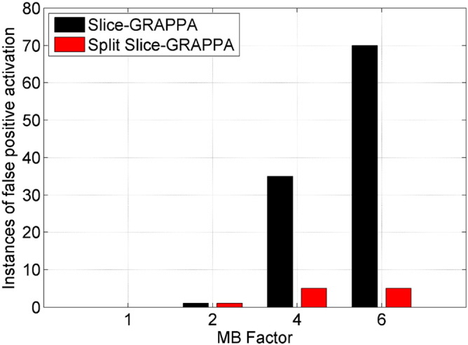
Summary of false-positive activations seen over all volunteers. For each MB factor and reconstruction type, the bar plots show the total number of confirmed instances of false-positive activation found over all ten volunteers.

Discussion

This study has demonstrated the data quality trade-offs involved as the combined acceleration factors (in plane and slice) are pushed higher and higher in a 1.5 mm isotropic whole-brain coverage imaging protocol at 3 T using a 32-channel head coil. The multiband approach offers a directly proportional improvement in temporal resolution, but the combined multiband and in-plane acceleration used in this study did not translate into improved BOLD sensitivity in a straight forward manner. The sensitivity results show significant gains in the motor and visual cortices for MB factors 2, 4, and 6 compared to MB factor 1. However, among these three higher MB factors, the peak sensitivity depends on anatomical location, which reconstruction method was used, and which metric is considered. As a disadvantage, imaging at high MB factors 4 or 6, combined with 2 × in-plane GRAPPA acceleration, can lead to false-positive activation arising from signal leaking between simultaneously excited slices when the data is reconstructed with the Slice-GRAPPA algorithm. This prevalence of false positives is greatly reduced when the same data is reconstructed using the Split Slice-GRAPPA method.

In order to properly assess the BOLD sensitivities of the data sets acquired with different MB factors, the evaluation had to account for the fact that the data sets had different sampling rates, numbers of samples, and temporal autocorrelations. This was done at the point of fitting the data to a general linear model (GLM) by using the FAST option in SPM12 for non-sphericity correction and the information was incorporated into both the tSNR_S metric and the t-score values such that each was directly proportional to the square root of the estimated number of degrees of freedom. The approach led to results for the tSNR_S values as a function of MB factor that closely reflected what was obtained for the two t-score metrics as a function of MB factor. When tSNR was calculated conventionally by taking the mean signal divided by standard deviation over time (i.e., ignoring the degrees of freedom), the results showed monotonically decreasing tSNR values as a function MB factor for each of the three anatomical regions considered. This conventional measure of tSNR demonstrates the lower image SNR at higher MB factors due to the reduced level of steady-state magnetization and the increased g-factor penalty. The increase in tSNR_S and t-score metrics at higher MB factors demonstrates the gain in statistical power due to the increased degrees of freedom in the data sets with more image volumes. The interaction between these opposing factors reduced image SNR, but more degrees of freedom appear as the primary drivers of the differences in BOLD sensitivity across the MB factors.

For a 2D multiband EPI sequence, the BOLD sensitivity is not expected to change homogeneously throughout the brain as a function of MB factor. The data acquisition is designed such that the same amount of raw data is acquired to form an image for any given MB factor. However, the ability of both reconstruction algorithms to separate the combined signals from the different slices and produce an accurate image depends on the geometry of the simultaneously excited slices and the coil sensitivity profiles. The interactions among the coil geometry, MB factor, and CAIPI shift can lead to complex spatial distributions of signal intensities. One example can be seen in the tSNR_S map for the MB 6 Slice-GRAPPA case shown in Fig. 1, where a band of high signal intensity appears near the parietal cortex that is not present in the MB 6 Split Slice-GRAPPA tSNR_S map. This increased tSNR_S is likely due to signal leaking from the high-intensity region of the occipital cortex, which was better suppressed with the Split Slice-GRAPPA reconstruction. This study considered performance metrics in three anatomical areas near the surface of the brain that each had relatively high SNR. The cerebellum had the lowest tSNR_S of the three areas, and it can be seen that the t-score metrics peak at MB 2 and drop significantly for MB 6 in this region. The performance at high MB factors is relatively worse for mid-brain regions where the coil sensitivity profiles are less optimal for signal separation and offer only low SNR, as can be seen in the lower tSNR_S in these areas.

Perhaps the most important result from this study is the clear evidence of false-positive activation seen in data sets acquired with total acceleration factors of 8 and 12 (MB factors 4 and 6 with in-plane GRAPPA 2) when reconstructed with the Slice-GRAPPA method. In these instances, the reconstruction algorithm was not able to fully separate the combined signal from several simultaneously excited slices. As a result, strong changes in the BOLD signal due to true positive activation originating from one physical location were aliased into other locations during the image reconstruction. The signal leakage was strong enough that these signal changes at the aliased locations were interpreted as activation by the statistical analysis. This is clearly unacceptable for fMRI studies where accurate localization of activation is of paramount importance.

As with the BOLD sensitivity metrics, the geometry of the brain, coil sensitivity profiles, and data acquisition scheme (MB factor and CAIPI shift) all play a role in the occurrence of false-positive activations. False-positive activation is most likely observed when a high activation in one region of the brain is aliased to locations that are in the center of the brain where the coil sensitivity profiles are suboptimal for signal separation. The example images shown in Fig. 6, Fig. 7 show that this situation is the case for activation clusters in the visual cortex. The use of in-plane GRAPPA 2 × acceleration leads to two possible alias locations per slice, separated by a distance of FOV/2, making it more likely that one the locations will fall in a region where greater signal leakage occurs. For studies that do not use in-plane acceleration, it may be possible to tailor the MB factor and CAIPI-shift parameters such that regions expected to have strong activation have strategically placed alias locations. For example, if the CAIPI-shift direction were reversed for the data in this study, many of the first adjacent slice alias locations from the visual cortex that produced false positives would be shifted outside the brain.

False-positive activation was seen not only in the simultaneously excited slice immediately adjacent to the true positive origination slice, but also sometimes in a location two slices away. Of the 106 instances of false-positive detection, there were 22 cases in which false positives were seen in more than one alias location. There were no instances of false-positive activation being detected in a location three slices or more away from the true activation origin. When considering an imaging protocol for high MB factors, it is advisable to consider the possible alias locations that will be closest to regions of likely high activation, as it is these locations that will have the greatest risk of false-positive activation. The closest alias location could be in an adjacent slice or directly above/below, depending on the MB factor and CAIPI shift used. Slice leakage maps (Fig. 9) may be helpful for this assessment.

The detection of false positives is aided by the fact that the alias locations of signal originating from a particular voxel can be precisely determined based on the knowledge of the MB factor and CAIPI shift used in the data acquisition. As done in this study, regions of true activation can be used as seed voxels to probe the known alias locations. If activation is detected at one of the alias locations, another criterion would need to be used to determine whether the activation is true or not. This study had four data sets for each volunteer in which the true activation should, in theory, be exactly the same, but the locations of the aliased false positives would be different. Therefore, activation seen at an alias location of one run, but not at the same location in the other three runs, could be considered to be false with high confidence. A study that does not contain repeated runs with different MB factors or CAIPI-shifts would need to use a different criterion, for example, activation at alias locations that are in white matter could be rejected as false (Schulz et al., 2014). If activation at an alias location falls in an area where activation could reasonably be expected to occur, it may not be possible to determine whether the activation is true or false.

The image reconstruction algorithm significantly affected the number of false positives detected. All of the above discussion was in reference to the Slice-GRAPPA reconstructed data, where 106 instances of false positives were confirmed. When the Split Slice-GRAPPA reconstruction was used on the same data, only 11 instances, across all scans of all subjects, of false-positive activation were found. This supports the better performance of Split Slice-GRAPPA in reducing signal leakage. However, it is possible that the lower SNR seen in the center of the brain with this reconstruction algorithm may have obscured false positives, leading to a relative overestimation of its performance. The procedure used for detecting instances of false-positive activation searched over a large number of voxels, ranging from 432 to 2,376 voxels. Given this large number of voxels searched and the threshold of p < 0.001 uncorrected, it is likely that some of the voxels exceeded the significance threshold by chance and were not false positives due to signal leakage. For example, assuming N samples drawn from the same binomial distribution with success probability of 0.001, the upper 95% confidence interval for the number of successes in N = 432 trials is 1.28, and for N = 2,376 trials, it is 7.03.

It is important to point out that most 3 T studies, which use more conventional resolutions of 2–3 mm, do not typically employ in-plane accelerations, nor is the need for it significant given the lower resolutions of those studies. Further, previous evaluations of MB signal leakage (Moeller et al., 2010, Xu et al., 2013) were evaluated as a function of separation between the bands, shift factors without in-plane accelerations, and using different FOVs (in plane and slice) and slice orientations than those employed here. All of these can significantly affect signal leakage across simultaneously excited slices. Further, the effectiveness and optimization of the CAIPI shift factor was not evaluated for the experimental conditions used in this work and the use of different shift factors may have altered the findings presented here. It is also not the case that the total acceleration factor (i.e., MB factor × GRAPPA factor) can be used to predict the corresponding fMRI performance, as an MB 8 × noGRAPPA is not equivalent to MB 4 × GRAPPA 2, despite having the same total acceleration factor. This is due to the fact that in-plane GRAPPA acceleration undersamples the data, giving a sqrt(R) penalty in SNR that is not present for MB accelerations. Lastly, we did not evaluate the case of MB 3 × GRAPPA 2 (i.e., total acceleration of 6), which may also be a viable alternative, especially when using the Split Slice-GRAPPA reconstruction.

This study necessarily considered a limited parameter space of MB accelerations, CAIPI-shift factors, reconstruction methods, and post-processing steps, in order to accommodate all measurements in a single scan session. Several other reconstruction methods for multiband data are described in the literature and may provide different trade-offs in performance than the two schemes presented here. These methods include SENSE/GRAPPA, 3D-GRAPPA, and SENSE (Breuer et al., 2005, Setsompop et al., 2012, Zahneisen et al., 2014, Zhu et al., 2012). Additionally, the effects of physiological noise and different physiological noise correction schemes were not considered. It is likely that the faster sampling rate of the higher MB factors used here would provide benefits in correcting for high frequency physiological noise sources.

Conclusion

A major limiting factor to performing high-resolution, whole-brain fMRI studies is the long scan time needed to acquire each image volume. Such studies could benefit considerably from the greatly improved temporal resolution provided by 2D multiband EPI sequences. The work presented here assessed the performance of a 2D multiband EPI sequence optimized for a 3 T scanner and 32-channel head coil with whole-brain coverage at 1.5 mm isotropic spatial resolution. The three major conclusions from the study are as follows: (1) imaging with multiband factor 2 and higher significantly improves BOLD sensitivity compared to the baseline unaccelerated case, (2) false-positive activation arising when BOLD signal changes due to true positive activation in one slice leak into other simultaneously excited slices can occur when using multiband factors of 4 or higher combined with in-plane accelerations, and (3) the choice of reconstruction algorithm has a significant effect on the level of false positive activation, with extensive false-positive activations almost entirely suppressed by the Split Slice-GRAPPA reconstruction. A very conservative approach for high-resolution whole-brain fMRI studies would be to use multiband acceleration factor 2, in-plane GRAPPA acceleration factor 2, and Split Slice-GRAPPA reconstruction. This approach affords significant improvements in BOLD sensitivity while avoiding false-positive activations due to slice leakage. Higher acceleration factors can be used (MB 3 or MB 4 × GRAPPA 2), but care must be taken to optimize the study design, imaging parameters, and reconstruction parameters in order to prevent the possibility of false-positive activations due to slice leakage.

References

- Ashburner J., Friston K.J. Unified segmentation. NeuroImage. 2005;26:839–851. doi: 10.1016/j.neuroimage.2005.02.018. [DOI] [PubMed] [Google Scholar]
- Bishop J.E., Plewes D.B. TE interleaving: new multisection imaging technique. J. Magn. Reson. Imaging. 1991;1:531–538. doi: 10.1002/jmri.1880010505. [DOI] [PubMed] [Google Scholar]
- Breuer F.A., Blaimer M., Heidemann R.M., Mueller M.F., Griswold M.A., Jakob P.M. Controlled aliasing in parallel imaging results in higher acceleration (CAIPIRINHA) for multi-slice imaging. Magn. Reson. Med. 2005;53:684–691. doi: 10.1002/mrm.20401. [DOI] [PubMed] [Google Scholar]
- Cauley S.F., Polimeni J.R., Bhat H., Wald L.L., Setsompop K. Interslice leakage artifact reduction technique for simultaneous multislice acquisitions. Magn. Reson. Med. 2014;72:93–102. doi: 10.1002/mrm.24898. [DOI] [PMC free article] [PubMed] [Google Scholar]
- Crooks L., Arakawa M., Hoenninger J., Watts J., McRee R., Kaufman L., Davis P.L., Margulis A.R., DeGroot J. Nuclear magnetic resonance whole-body imager operating at 3.5 KGauss. Radiology. 1982;143:169–174. doi: 10.1148/radiology.143.1.7063722. [DOI] [PubMed] [Google Scholar]
- Deichmann R., Schwarzbauer C., Turner R. Optimisation of the 3D MDEFT sequence for anatomical brain imaging: technical implications at 1.5 and 3 T. NeuroImage. 2004;21:757–767. doi: 10.1016/j.neuroimage.2003.09.062. [DOI] [PubMed] [Google Scholar]
- Eickhoff S.B., Stephan K.E., Mohlberg H., Grefkes C., Fink G.R., Amunts K., Zilles K. A new SPM toolbox for combining probabilistic cytoarchitectonic maps and functional imaging data. NeuroImage. 2005;25:1325–1335. doi: 10.1016/j.neuroimage.2004.12.034. [DOI] [PubMed] [Google Scholar]
- Feinberg D.A., Setsompop K. Ultra-fast MRI of the human brain with simultaneous multi-slice imaging. J. Magn. Reson. 2013;229:90–100. doi: 10.1016/j.jmr.2013.02.002. [DOI] [PMC free article] [PubMed] [Google Scholar]
- Feinberg D.A., Yacoub E. The rapid development of high speed, resolution and precision in fMRI. NeuroImage. 2012;62:720–725. doi: 10.1016/j.neuroimage.2012.01.049. [DOI] [PMC free article] [PubMed] [Google Scholar]
- Feinberg D.A., Reese T.G., Wedeen V.J. Simultaneous echo refocusing in EPI. Magn. Reson. Med. 2002;48:1–5. doi: 10.1002/mrm.10227. [DOI] [PubMed] [Google Scholar]
- Feinberg D.A., Moeller S., Smith S.M., Auerbach E., Ramanna S., Gunther M., Glasser M.F., Miller K.L., Ugurbil K., Yacoub E. Multiplexed echo planar imaging for sub-second whole brain FMRI and fast diffusion imaging. PLoS One. 2010;5:e15710. doi: 10.1371/journal.pone.0015710. [DOI] [PMC free article] [PubMed] [Google Scholar]
- Friston K.J., Glaser D.E., Henson R.N., Kiebel S., Phillips C., Ashburner J. Classical and Bayesian inference in neuroimaging: applications. NeuroImage. 2002;16:484–512. doi: 10.1006/nimg.2002.1091. [DOI] [PubMed] [Google Scholar]
- Friston K.J., Ashburner J., Kiebel S., Nichols T., Penny W.D. Elsevier; 2007. Statistical Parametric Mapping: The Analysis of Functional Brain Images. [Google Scholar]
- Larkman D.J., Hajnal J.V., Herlihy A.H., Coutts G.A., Young I.R., Ehnholm G. Use of multicoil arrays for separation of signal from multiple slices simultaneously excited. J. Magn. Reson. Imaging. 2001;13:313–317. doi: 10.1002/1522-2586(200102)13:2<313::aid-jmri1045>3.0.co;2-w. [DOI] [PubMed] [Google Scholar]
- Lin F.H., Tsai K.W., Chu Y.H., Witzel T., Nummenmaa A., Raij T., Ahveninen J., Kuo W.J., Belliveau J.W. Ultrafast inverse imaging techniques for fMRI. NeuroImage. 2012;62:699–705. doi: 10.1016/j.neuroimage.2012.01.072. [DOI] [PMC free article] [PubMed] [Google Scholar]
- Loenneker T., Hennel F., Hennig J. Multislice interleaved excitation cycles (MUSIC): an efficient gradient-echo technique for functional MRI. Magn. Reson. Med. 1996;35:870–874. doi: 10.1002/mrm.1910350613. [DOI] [PubMed] [Google Scholar]
- Lutti A., Thomas D.L., Hutton C., Weiskopf N. High-resolution functional MRI at 3 T: 3D/2D echo-planar imaging with optimized physiological noise correction. Magn. Reson. Med. 2013;69:1657–1664. doi: 10.1002/mrm.24398. [DOI] [PMC free article] [PubMed] [Google Scholar]
- Moeller S., Yacoub E., Olman C.A., Auerbach E., Strupp J., Harel N., Ugurbil K. Multiband multislice GE-EPI at 7 Tesla, with 16-fold acceleration using partial parallel imaging with application to high spatial and temporal whole-brain fMRI. Magn. Reson. Med. 2010;63:1144–1153. doi: 10.1002/mrm.22361. [DOI] [PMC free article] [PubMed] [Google Scholar]
- Neggers S.F., Hermans E.J., Ramsey N.F. Enhanced sensitivity with fast three-dimensional blood-oxygen-level-dependent functional MRI: comparison of SENSE-PRESTO and 2D-EPI at 3 T. NMR Biomed. 2008;21:663–676. doi: 10.1002/nbm.1235. [DOI] [PubMed] [Google Scholar]
- Nunes R., Hajnal J.V., Golay X., Larkman D.J. Proceedings of the 14th annual meeting of ISMRM, Seattle, Washington, USA. 2006. Simultaneous slice excitation and reconstruction for single shot EPI. [Google Scholar]
- Poser B.A., Koopmans P.J., Witzel T., Wald L.L., Barth M. Three dimensional echo-planar imaging at 7 Tesla. NeuroImage. 2010;51:261–266. doi: 10.1016/j.neuroimage.2010.01.108. [DOI] [PMC free article] [PubMed] [Google Scholar]
- Posse S., Ackley E., Mutihac R., Rick J., Shane M., Murray-Krezan C., Zaitsev M., Speck O. Enhancement of temporal resolution and BOLD sensitivity in real-time fMRI using multi-slab echo-volumar imaging. NeuroImage. 2012;61:115–130. doi: 10.1016/j.neuroimage.2012.02.059. [DOI] [PMC free article] [PubMed] [Google Scholar]
- Schulz J., Siegert T., Bazin P.L., Maclaren J., Herbst M., Zaitsev M., Turner R. Prospective slice-by-slice motion correction reduces false positive activations in fMRI with task-correlated motion. NeuroImage. 2014;84:124–132. doi: 10.1016/j.neuroimage.2013.08.006. [DOI] [PubMed] [Google Scholar]
- Setsompop K., Gagoski B.A., Polimeni J.R., Witzel T., Wedeen V.J., Wald L.L. Blipped-controlled aliasing in parallel imaging for simultaneous multislice echo planar imaging with reduced g-factor penalty. Magn. Reson. Med. 2012;67:1210–1224. doi: 10.1002/mrm.23097. [DOI] [PMC free article] [PubMed] [Google Scholar]
- Smith S.M., Beckmann C.F., Andersson J., Auerbach E.J., Bijsterbosch J., Douaud G., Duff E., Feinberg D.A., Griffanti L., Harms M.P., Kelly M., Laumann T., Miller K.L., Moeller S., Petersen S., Power J., Salimi-Khorshidi G., Snyder A.Z., Vu A.T., Woolrich M.W., Xu J., Yacoub E., Ugurbil K., Van Essen D.C., Glasser M.F., Consortium W.U.-M.H. Resting-state fMRI in the Human Connectome Project. NeuroImage. 2013;80:144–168. doi: 10.1016/j.neuroimage.2013.05.039. [DOI] [PMC free article] [PubMed] [Google Scholar]
- SPM12 SPM12 framework, Wellcome Trust Centre for Neuroimaging. http://www.fil.ion.ucl.ac.uk/spm/ (London)
- Swisher J.D., Sexton J.A., Gatenby J.C., Gore J.C., Tong F. Multishot versus single-shot pulse sequences in very high field fMRI: a comparison using retinotopic mapping. PLoS One. 2012;7:e34626. doi: 10.1371/journal.pone.0034626. [DOI] [PMC free article] [PubMed] [Google Scholar]
- Tijssen R.H., Okell T.W., Miller K.L. Real-time cardiac synchronization with fixed volume frame rate for reducing physiological instabilities in 3D FMRI. NeuroImage. 2011;57:1364–1375. doi: 10.1016/j.neuroimage.2011.05.070. [DOI] [PubMed] [Google Scholar]
- Tong Y., Frederick B. Tracking cerebral blood flow in BOLD fMRI using recursively generated regressors. Hum. Brain Mapp. 2014;35:5471–5485. doi: 10.1002/hbm.22564. [DOI] [PMC free article] [PubMed] [Google Scholar]
- Tong Y., Hocke L.M., Frederick B. Short repetition time multiband echo-planar imaging with simultaneous pulse recording allows dynamic imaging of the cardiac pulsation signal. Magn. Reson. Med. 2014;72:1268–1276. doi: 10.1002/mrm.25041. [DOI] [PMC free article] [PubMed] [Google Scholar]
- Xu J., Moeller S., Auerbach E.J., Strupp J., Smith S.M., Feinberg D.A., Yacoub E., Ugurbil K. Evaluation of slice accelerations using multiband echo planar imaging at 3 T. NeuroImage. 2013;83:991–1001. doi: 10.1016/j.neuroimage.2013.07.055. [DOI] [PMC free article] [PubMed] [Google Scholar]
- Zahneisen B., Ernst T., Poser B.A. SENSE and simultaneous multislice imaging. Magn. Reson. Med. 2014 doi: 10.1002/mrm.25519. (Epub ahead of print) [DOI] [PMC free article] [PubMed] [Google Scholar]
- Zhu K., Kerr A., Pauly J. Proceedings of the 20th Annual Meeting of the ISMRM, Melbourne, Australia. 2012. Autocalibrating CAIPIRINHA: Reformulating CAIPIRINHA as a 3d problem; p. 518. [Google Scholar]