

Abstract
Over the past several years, the death rate associated with drug poisoning has increased by over 300% in the U.S. Drug poisoning mortality varies widely by state, but geographic variation at the substate level has largely not been explored. National mortality data (2007–2009) and small area estimation methods were used to predict age-adjusted death rates due to drug poisoning at the county level, which were then mapped in order to explore: whether drug poisoning mortality clusters by county, and where hot and cold spots occur (i.e., groups of counties that evidence extremely high or low age-adjusted death rates due to drug poisoning). Results highlight several regions of the U.S. where the burden of drug poisoning mortality is especially high. Findings may help inform efforts to address the growing problem of drug poisoning mortality by indicating where the epidemic is concentrated geographically.
Keywords: Empirical Bayes prediction, Spatial variation, Overdose, Cold spots
1. Introduction
The burden of mortality and morbidity associated with drug poisoning represents a growing public health concern in the U.S. Poisoning has recently overtaken motor vehicle crashes as the leading cause of injury death in the U.S.; the death rate associated with drug poisoning has increased by approximately 300% over the past several decades (Warner et al., 2011). Increases in deaths due to opioid analgesics have been particularly large for U.S. women, rising by 415% since 1999 (Centers for Disease Control and Prevention, 2013). Opioid analgesics contribute to more than three in four poisoning deaths; and the use and misuse of prescription drugs, particularly opioid analgesics, has increased in parallel with drug poisoning mortality (Centers for Disease Control and Prevention, 2011, 2013). There is wide variation at the state level with respect to age-adjusted drug poisoning death rates (Centers for Disease Control and Prevention, 2011; Paulozzi and Ryan, 2006; Warner et al., 2011). Extremely high annual rates have been observed for New Mexico (30.8 per 100,000), West Virginia (27.6 per 100,000), Alaska (24.2 per 100,000), Nevada (21.0 per 100,000), and Utah (20.8 per 100,000) (Centers for Disease Control and Prevention, 2011; Warner et al., 2011). However, variation within states has largely not been examined.
A few studies have looked at variation at the sub-state level, but have focused on limited geographic areas such as New York City, Rhode Island, North Carolina, New Hampshire and Connecticut (Cerdá et al, 2013; DiMaggio et al., 2008; Green and Donnelly, 2011; Green et al., 2011; Hester et al., 2012; Modarai et al., 2013). Some studies have suggested that drug poisoning mortality disproportionately affects rural areas as compared to urban (Paulozzi and Xi, 2008), but it is possible that urban–rural differences may be influenced by underlying geographic or regional patterns. The objectives of this study were to use spatial statistical tools to examine county-level variation in drug poisoning mortality and highlight areas of the U.S. where drug-related poisoning deaths are higher or lower than expected, with the goal of informing efforts to address this growing epidemic.
2. Materials and methods
2.1. Data and empirical Bayes estimates
Data on drug poisoning deaths were obtained from the 2007–2009 National Vital Statistics Multiple Cause of Death Files (Kochanek et al., 2011; Minino et al., 2011). Deaths were classified using the International Classification of Diseases (ICD), Tenth Revision (ICD-10). Age-adjusted death rates (AADR) due to drug poisoning were calculated by county and year using the direct method and the 2000 standard population (Kochanek et al., 2011; Minino et al., 2011). Since drug poisoning deaths are a rare event, calculating county-level drug poisoning death rates based on crude rates will produce highly unstable estimates. We therefore used small area estimation techniques to produce stable county-level estimates of age-adjusted death rates (AADR) associated with drug poisoning for 3141 counties in the U.S., 2007–2009. Small area estimation techniques are increasingly being used in disease mapping to produce reliable estimates for areas where population sizes are small or events are infrequent. We review these methods briefly here. Details on the methods can be found in Supplemental Appendix A and has been recently described elsewhere (Rossen et al., 2013).
Two-stage mixed effects models were used to estimate county-level drug poisoning AADRs, due to the highly non-normal distribution of poisoning death rates which are highly zero-inflated and right-skewed (Afifi et al., 2007; Alfo and Maruotti, 2010; Baughman, 2007; Kowalski et al., 2003; Li et al., 2011; Wang, 2010; Xie et al., 2004), as approximately 24% of counties had zero deaths in any given year. The first stage modeled the probability of observing no deaths, and the second stage modeled the expected log-transformed age-adjusted death rate, conditional on having a death. Mixed effects models are commonly used in small area estimation, as they can be used to predict empirical Bayes estimates which borrow information across clusters to shrink extreme values and provide stable small area estimates (Pfefferman, 2002; Rao, 2003; Saei and Chambers, 2003; Skrondal and Rabe-Hesketh, 2009).
We included county-level random intercepts and fixed effects in both steps of the model using the Generalized Linear and Latent Mixed Modeling (GLLAMM) procedures in Stata 12.1 SE (Rabe-Hesketh et al., 2004; StataCorp, 2011). Fixed effects included a variety of county-level covariates drawn from several sources, including socio-demographic and economic characteristics, crime, urban–rural classification, and health-related data (Federal Bureau of Investigation, 2000), National Center for Health Statistics Urban–Rural Classification Scheme (Ingram and Franco, 2012) and the decennial Census of the U.S. population (U.S. Department of Commerce, Bureau of the Census, 2000)) for the year 2000. A list of included covariates can be seen in Table 1.
Table 1.
Covariates included in empirical Bayes estimate modeling of age-adjusted death rates due to drug poisoning in the U.S., 2007–2009.
| Region of the country (Division: New England, Mid-Atlantic, East North Central, West North Central, South Atlantic, East South Central, West South Central, Mountain, Pacific) | Median age |
|---|---|
| Percent black | |
| Percent white | |
| Percent Hispanic | |
| Latitude and longitude of county centroid Square miles | Percent Asian Percent other race |
| Population size | Percent with less than HS education |
| Residential density | Percent female headed households |
| Percent rural | Number of MDs |
| Percent of land that is farm | Number of hospitals |
| Median home value | Percent on medicare |
| Percent household public assistance | Percent on medicaid |
| Percent renter occupied housing | Number in jail |
| Percent households with dividend income | Number in juvenile detention |
| Percent English speaking | Number homeless |
| Percent native | Average percent humidity in July |
| Percent households without earnings | Above the median arrests for drug sale |
| Above the median arrests for drug-related crimes | Percent unemployed |
| Central, fringe, medium metropolitan, micropolitan, non-core/rural Percent of deaths with pending causes | |
| Proportion of population reporting nonmedical prescription drug use | |
Metropolitan counties were classified to one of four levels based on the population size and proximity to urban centers: large core and large fringe (population >1 million); medium (population 250,000–999,999); and small (population <250,000). Non-metropolitan counties were classified as micropolitan or non-core. In this analysis, rural refers to non-core counties. Additionally, models included the estimated proportions of the population reporting nonmedical use of prescription medication as assessed by the National Survey on Drug Use and Health obtained from the Substance Abuse and Mental Health Services Administration for 344 substate regions, 2007–2008 (Substance Abuse and Mental Health Services Administration, 2009). Finally, the percent of deaths for which the final cause of death was pending (at the state level) was also included because poisonings account for a large proportion of pending deaths (Warner and Chen, 2012). The posterior predictions from each stage of the model incorporate both an empirical Bayes estimate for each county, plus the linear (or log-linear) prediction from the fixed effects portions of the models (Skrondal and Rabe-Hesketh, 2009). This auxiliary information was included to improve the predictive power of the models (Pfefferman, 2002; Saei and Chambers, 2003). Overall, 74% of the between-county variance in the likelihood of reporting at least one drug poisoning fatality was explained by the included covariates, as was 42% of the between-county variance in the age-adjusted death rates due to drug poisoning. County-level drug poisoning AADRs were then estimated by multiplying the predicted posterior probability of having a death obtained from the first step with the posterior mean drug-related AADR obtained from the second step. These predicted drug poisoning AADRs were then merged with U.S. Census Tiger/Line files and mapped using ArcGIS 10.1 (ESRI, 2011).
2.2. Spatial statistical tools
2.2.1. Global index of spatial autocorrelation – Moran’s I
Global indexes of spatial autocorrelation were used to assess the similarity, or spatial dependence, across counties with respect to drug poisoning mortality. In other words, do counties with similar drug poisoning AADRs tend to be located close together or are drug poisoning AADRs randomly distributed across counties in the U.S.? The Global Moran’s I statistic is evaluated in terms of a null hypothesis that AADRs by county are spatially random (ESRI, 2011; Waller and Gotway, 2004). From Waller and Gotway (2004), the Global Moran’s I statistic for spatial autocorrelation is given as
where zi is the deviation (xi−X) of AADR’s for county i from the overall mean, ωij is the spatial weight between county i and j (described below), n is equal to the total number of counties, and SO is the aggregate of all the spatial weights:
The zi-score for the statistic is
where E[I] = −1/(n − 1) and V[I] = E[I2] − E[I]2.
High values of the Moran’s I and corresponding z-scores greater than −1.96 indicate that there is statistically significant clustering across the study area (p < 0.05). Low values of the Moran’s I and z-scores less than −1.96 indicate that there is statistically significant regularity (nearby counties have very different AADRs). Moran’s I can be thought of as a spatially weighted form of Pearson’s correlation coefficient (Waller and Gotway, 2004).
2.2.2. Conceptualization of spatial relationships
There are several ways to define ωij, the spatial weight between county i and j. We explored three methods, inverse distance, K nearest neighbors and Delaunay triangulation. In the inverse distance conceptualization, every county is assumed to be a neighbor of every other county, and the influence of counties decays with increasing distance (ESRI, 2011). Since our study area consisted of the entire U.S., this conceptualization is problematic because large distances between counties result in very small weights and “salt-and-pepper” style maps. Additionally, the heterogeneity in county sizes across the U.S. leads to small counties with close neighbors being given greater weight than larger counties with neighbors that are farther away. To circumvent the issue of heterogeneous county sizes and the large study area, we explored the K nearest neighbors option, where a general rule of thumb is to evaluate each county in the context of a minimum of eight neighbors (ESRI, 2011). However, because we found several isolated counties with fewer than eight neighbors (i.e., some counties in Hawaii and Alaska), we ultimately proceeded with the Delaunay triangulation conceptualization of spatial relationships. Delaunay triangulation specifies natural neighbors for a set of counties by creating Voronoi triangles from county centroids; nodes connected by a triangle edge are considered neighbors. Fig. 1 illustrates the Delaunay triangulation method.
Fig. 1.

Example of Delaunay triangulation. Counties in light gray are considered neighbors of the county shaded dark gray.
This method works well when there are isolated features or heterogeneity in county size (ESRI, 2011). This method ensures that every county has at least one neighbor but utilizes the distribution of the data for determining how many neighbors each county gets. We created a spatial weights matrix file using the Delaunay triangulation conceptualization of spatial relationships. Sensitivity analyses were conducted using the eight-nearest-neighbors conceptualization.
2.2.3. Local indicators of spatial association – Getis-Ord
While global indexes of spatial autocorrelation assess whether there is clustering across the study area, local indicators of spatial association can be used to identify specific clusters of high or low drug poisoning AADRs (Waller and Gotway, 2004). We used the Getis-Ord statistic to identify significant clusters of counties with high or low AADRs (ESRI, 2011). The Getis-Ord statistic generates a z-score and corresponding p-value for each data point, where z-scores greater than −1.96 indicate a significant “hot spot” and z-scores lower than 1.96 indicate a significant “cold spot” (p < 0.05). From ESRI (2011), the Getis-Ord statistic is calculated as
where xj is the AADR’s for each county j, ωij is the spatial weight between county i and j, n is equal to the total number of features and
and
3. Results
The predicted mean county-level AADR for the years 2007–2009 was 30.76 per 100,000 population (SD: 16.08), and ranged from a low of 0.45 to a high of 128.48 per 100,000 population. The raw county-level AADRs ranged from 0 to 222.4 per 100,000 population (SD: 26.5). The differences between the range in estimated AADRs and the raw rates were small; however, the estimated AADRs were much less variable. Fig. 2 depicts the predicted drug poisoning AADRs across 3141 counties for the years 2007–2009. Approximately 7.64% of counties had AADRs less than 10 per 100,000 population, while 11.37% of counties had AADRs greater than 50 per 100,000 population.
Fig. 2.
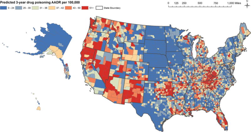
Predicted drug poisoning AADR by county, 2007–2009.
3.1. Clustering of drug poisoning mortality – Moran’s I
The Global Moran’s I was 0.55, with a corresponding z-score of 53.53, suggesting that there was significant spatial autocorrelation of county-level drug poisoning AADRs (p < 0.05). In other words, across the U.S., counties with similar drug poisoning AADRs tend to locate closer to one another than we would expect by random chance.
3.2. Hot and cold spots – Getis-Ord
Significant clusters of counties with high (hot spots) and low (cold spots) AADRs, as assessed by the Getis-Ord tool can be seen in Fig. 3.
Fig. 3.
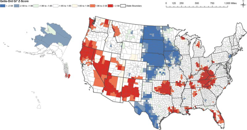
Hot and cold spots in drug poisoning mortality, 2007–2009
Sensitivity analyses using eight-nearest-neighbors produced very similar results (not shown). While some previous studies have suggested that drug poisoning AADRs are higher in rural areas as compared to more urban areas, we observed significant hot spots and cold spots in rural areas. Significant hot spots were seen along the North Pacific coast (i.e., northern California, Washington), the Southwest (i.e., Nevada, Arizona and New Mexico), Oklahoma, Appalachia (i.e., areas of Kentucky, Tennessee, West Virginia, Virginia, North Carolina), and the Gulf coast (i.e., the coast of Louisiana, Mississippi, and Florida). Cold spots were identified across the Central Plains (i.e., North and South Dakota, Nebraska, Kansas), Texas, and regions of Alaska. Results indicate that rural areas represent both hot and cold spots in drug poisoning death rates. Rural areas across the Central Plains states, Texas, and Alaska represent significant cold spots; while rural areas in Appalachia, Northern California, Oklahoma, and New Mexico represent significant hot spots.
4. Discussion
There is substantial geographic variation in age adjusted death rates (AADR) due to drug poisoning across the U.S. Results of global tests of spatial autocorrelation (i.e., Moran’s I) confirm that drug poisoning mortality exhibits spatial dependence. In other words, across the entire U.S., counties with high drug poisoning AADRs tend to locate closer together than we would expect at random. Conversely, counties with low levels of drug poisoning mortality also tend to cluster together geographically. Using local indicators of spatial association (i.e., Getis Ord ), we were able to identify several hot and cold spots across the U.S. that represent clusters of counties with significantly high or low drug poisoning death rates. The main hot spots detected occurred along the North Pacific coast (i.e., northern California, Washington), the Southwest (i.e., Nevada, Arizona and New Mexico), Oklahoma, Appalachia (i.e., areas of Kentucky, Tennessee, West Virginia, Virginia, North Carolina), and the Gulf coast (i.e., the coast of Louisiana, Mississippi, and Florida). Cold spots were identified across the Central Plains (i.e., North and South Dakota, Nebraska, Kansas), Texas, and regions of Alaska.
Previous research has indicated that drug poisoning mortality is a major concern for rural areas, and particularly for Appalachia (Centers for Disease Control and Prevention, 2011; Frosch, 2012; Hiaasen, 2009; Paulozzi and Ryan, 2006; Rossen et al., 2013; Wunsch et al., 2009). Our results are partially consistent with these patterns, as we did observe a hot spot of extremely high death rates due to drug poisoning in the Appalachian region. Hot spots were also observed for rural regions of Northern California, New Mexico, Oklahoma, Arkansas, and Michigan. However, we also observed cold spots, or significantly low AADRs due to drug poisoning, across large swaths of rural counties in the central U.S. For example, cold spots in North and South Dakota, Nebraska, Kansas, Minnesota, Iowa, and Texas were predominantly in rural areas. In contrast to previous research suggesting that drug poisoning mortality is disproportionately high in rural areas as opposed to more urban areas; our results indicate that rural areas of the U.S. represented some of the lowest and highest drug poisoning death rates. As previous research has largely not examined spatial variation in drug poisoning mortality, results of this study highlight that the variation in drug poisoning mortality appears to be influenced heavily by geography as opposed to just urban–rural classification. One analysis of opioid-related deaths in New Hampshire reported that there was significant clustering of poisoning deaths across Zip Code Tabulation Areas, and that death rates were associated with lower area income levels and higher rates of employment-related disability, but not with rural status (Hester et al., 2012). Hester et al. (2012) suggested that geographic factors such as proximity to regions where opioids are highly available might be more critical to spatial patterning than population density.
Substantial geographic variation in drug poisoning mortality was apparent, as clear clusters of counties with extremely high and low drug poisoning AADRs emerged. These clusters often crossed state borders, as could be seen in the Appalachian region and the hot spots across the Pacific coast and Southwest U.S., as well as the large cold spots that were seen in the central U.S. More research is needed to explore the drivers of these geographic patterns, as it remains unclear why certain areas of the U.S. are experiencing extremely high (or low) drug poisoning death rates. A variety of regional-, county-, or neighborhood-level characteristics could be associated with geographic variation in drug poisoning mortality. A recent analysis reported that the amount of opioids prescribed was highest in Nevada, Florida and the Appalachian states; similar to some of the geographic patterns in drug poisoning mortality observed in this study (McDonald et al., 2012). Maps of the prevalence of nonmedical use of pain relievers from the National Survey of Drug Use and Health also overlap with drug poisoning mortality in many areas (Substance Abuse and Mental Health Services Association, 2012). For example, states on the Pacific Coast, South West, and Oklahoma have reported high prevalence rates of nonmedical use of pain relievers, while North and South Dakota have relatively low prevalence rates. A spatial analysis of hot and cold spots of drug use in the U.S. (also using data from the National Survey of Drug Use and Health) generated results that are similar in some regards to those described in the present analysis (Gopal et al., 2008). For example, North and South Dakota appeared to represent cold spots when mapping rates of abuse or dependence on illicit drugs (excluding marijuana), while hot spots were identified in parts of California, the South West, Oklahoma, and some Appalachian states (Gopal et al., 2008). However, that analysis also suggested that parts of Texas represented a hot spot, and also identified Pennsylvania and Maryland as cold spots, in contrast to the present study of drug poisoning mortality. Results may differ for several reasons. Gopal et al. (2008) utilized data from 2002 to 2004 and patterns may have changed over time, self-report data may produce different spatial patterns as compared to data from death certificates, and/or geographic variation in drug abuse or dependence may not cohere with that of mortality due to drug poisoning. As few studies have looked at variation at the sub-state level (Cerdá et al., 2013; DiMaggio et al., 2008; Green and Donnelly, 2011; Green et al, 2011; Hester et al., 2012; Modarai et al., 2013; Rossen et al., 2013) the drivers of spatial variation in drug poisoning mortality remain unclear. Further research is needed to elucidate the causal factors that contribute to these geographic patterns.
This study has a few limitations. It is possible that drug poisoning deaths were underestimated. There are many challenges to accurately classifying deaths due to drug poisoning and compiling this information on a national scale; a process which relies heavily on professional judgment and varying levels of evidence and resources available to medical examiners and coroners (Davis, 2013; Prescription Monitoring Program Center of Excellence at Brandeis, 2011; Szalavitz, 2010; Warner et al., 2013). Therefore, there may be some misclassification bias when using federal vital statistics to examine drug poisoning deaths (Dasgupta et al., 2008). Poisoning deaths are disproportionately represented among the cases where the cause of death remains pending in the death certificate data, so although we included the percent of pending cases at the state level as a covariate in our models, it is possible that pending cause of death disproportionately represents drug poisoning mortality and varies by county; additionally, other types of misclassification may vary geographically, potentially affecting our examinations of county-level spatial variation (Dasgupta et al., 2008; Landen et al., 2003). This kind of misclassification would be more likely to contribute to the incorrect identification of cold spots, though it could also result in the failure to detect a hot spot particularly in sparsely populated areas where a single death can substantially influence the AADR for that county. The purpose of using small area estimation techniques was to stabilize these extreme or unreliable values. The advantage of using small area estimation is that information is ‘borrowed’ across units to produce reliable estimates when only small samples are available in certain areas, such as in rural counties. The inclusion of various covariates derived from many data sources served to improve these predictions, and explained a large portion of the between-county variance in the likelihood of observing a drug poisoning fatality and the age-adjusted death rate due to drug poisoning. However, there was a degree of unexplained variance, which could be the result of residual spatial variation or omitted variables such as access to various types of drugs, or other factors related to local drug markets, physician prescribing patterns, or the prevalence of doctor-shopping or drug-diversion (National Research Council, 2010; Paulozzi and Ryan, 2006). Future studies should examine these potential determinants to explore whether these factors may help to explain some of the clusters of extremely high drug poisoning death rates observed in this study.
Future studies should also explore spatial patterns by type of drug, as findings may differ for illicit or prescription drugs (Cerdá et al, 2013; Dasgupta et al., 2008; Hester et al., 2012; National Research Council, 2010). As this study examined drug poisoning overall, it remains unclear how spatial patterns by drug type might overlap or remain distinct, and how the overall spatial patterning might be influenced. For example, a report on drug poisonings in Connecticut reported that heroin fatalities were more likely to occur in urban areas, while prescription opioid fatalities were more likely to occur in small towns (Green et al., 2011). Dasgupta et al. (2008) reported distinct geographic patterns for heroin overdoses as compared to prescription opioid deaths, and variation between metropolitan and non-metropolitan areas in death rates due to alcohol, benzodiazepines, antidepressants, prescription opioids, and illicit drugs. Recent studies have also shown that there are changes in drug use patterns with nonmedical users of prescription opioids transitioning to heroin use (Jones, 2013). For the purposes of this analysis, we examined overall drug poisoning mortality for two reasons. First, because previous studies have reported that the classification of deaths due to a specific drug are more prone to error than categorizing overall drug poisoning in vital statistics (Landen et al., 2003). Second, because the specific drug type was not available for 25% of the drug poisoning deaths, and it varied by state, ranging from approximately 65% to less than 1% missing data (Warner et al., 2013).
Finally, there is no ideal characterization of spatial relationships when analyzing hot spots, particularly when examining a large geographic region such as the entire U.S. Due to the presence of several island counties in Hawaii and Alaska and general unevenness of county size (in terms of geographic area), we used Delaunay triangulation, which creates weights based on a county’s natural neighbors and ensures every county has a least one neighbor. We also ran analyses using eight nearest neighbors, which produced results largely similar to those reported here. However, there are alternative characterizations that could be explored, such dividing the U.S. into regions and examine each separately to ensure some consistency in county size. While counties may not be the ideal unit to examine drug poisoning mortality, as there is likely substantial variation at the sub-county level, the data are compiled for the nation by county. Results are subject to potential biases related to the modifiable areal unit problem and ecological fallacies (Holt et al., 1996).
This study has a number of strengths. We used small area estimation techniques to generate stable estimates of age adjusted death rates due to drug poisoning at the county level. It is the first study to highlight spatial clusters of high and low drug poisoning death rates in the U.S. and was able to identify hot or cold spots that span multiple states. Previous studies have focused on limited geographic areas such as a single state (Cerdá et al, 2013; DiMaggio et al., 2008; Green and Donnelly, 2011; Modarai et al., 2013), have not used small area estimation methods, or spatial statistical tools to examine geographic variation in drug poisoning mortality across the U.S.
5. Conclusions
In sum, there is substantial geographic variation in drug poisoning mortality across the U.S. Counties with high and low death rates due to drug poisoning tend to cluster together more than we would expect by chance. Several hot spots were detected, notably, Appalachia, areas of Northern California, Nevada, Arizona and New Mexico, Oklahoma, Florida, and parts of the Gulf Coast. Cold spots were observed across the North-Central U.S., and parts of Texas. As rural areas contributed to both hot and cold spots, no uniform pattern emerged by rural or urban classification. Examining geographic variation in drug poisoning death rates is critical to future efforts aimed at understanding and targeting this growing epidemic.
Supplementary Material
Appendix A. Supplementary material
Supplementary data associated with this article can be found in the online version at http://dx.doi.org/10.1016/j.healthplace.2013.11.005.
Footnotes
Disclaimer
The findings and conclusions in this paper are those of the author(s) and do not necessarily represent the official position of the National Center for Health Statistics, Centers for Disease Control and Prevention.
References
- Afifi AA, Kotlerman JB, Ettner SL, Cowan M. Methods for improving regression analysis for skewed continuous or counted responses. Annu Rev Public Health. 2007;28:95–111. doi: 10.1146/annurev.publhealth.28.082206.094100. [DOI] [PubMed] [Google Scholar]
- Alfo M, Maruotti A. Two-part regression models for longitudinal zero-inflated count data. Can J Stat. 2010;38(2):197–216. [Google Scholar]
- Baughman AL. Mixture model framework facilitates understanding of zero-inflated and hurdle models for count data. J Biopharm Stat. 2007;17(5):943–946. doi: 10.1080/10543400701514098. [DOI] [PubMed] [Google Scholar]
- Centers for Disease Control and Prevention. Vital signs: overdoses of prescription opioid pain relievers—United States, 1999–2008. Morb Mortal Wkly Rep. 2011;60(43):1487–1492. [PubMed] [Google Scholar]
- Centers for Disease Control and Prevention. Vital signs: overdoses of prescription opioid pain relievers and other drugs among women – United States, 1999–2010. Morb Mortal Wkly Rep. 2013;62(26):537–542. [PMC free article] [PubMed] [Google Scholar]
- Cerdá M, Ransome Y, Keyes KM, Koenen KC, Tracy M, Tardiff KJ, Vlahov D, Galea S. Prescription opioid mortality trends in New York City, 1990–2006: examining the emergence of an epidemic. Drug Alcohol Depend. 2013 doi: 10.1016/j.drugalcdep.2012.12.027. http://dx.doi.org/10.1016/j.drugalcdep.2012.12.027. [DOI] [PMC free article] [PubMed]
- Dasgupta N, Jönsson Funk M, Brownstein J. Comoparing unintentional opioid poisoning mortality in metropolitan and non-metropolitan counties, United States, 1999–2003. In: Thomas Y, Richardson D, Cheung I, editors. Geography and Drug Addiction. Springer; New York: 2008. [Google Scholar]
- Davis GG. the National Association of Medical Examiners and American College of medical Toxicology Expert Panel on Evaluating and Reporting Opioid Deaths, 2013. National Association of Medical Examiners Position Paper: recommendations for the investigation, diagnosis and certification of deaths related to opioid drugs. Acad Forensic Pathol. 2013;3(1):77–83. [Google Scholar]
- DiMaggio CJ, Bucciarelli A, Tardiff KJ, Vlahov D, Galea S. Spatial analytic approaches to explaining the trends and patterns of drug overdose deaths. In: Thomas Y, Richardson D, Cheung I, editors. Geography and Drug Addiction, 2008. Springer; New York, Dordrecht: 2008. pp. 447–464. http://dx.doi.org/10.1007/978-1-4020-8509-3-27. [Google Scholar]
- ESRI. ArcGIS Desktop: Release 10. Environmental Systems Research Institute; Redlands, CA: 2011. [Google Scholar]
- Federal Bureau of Investigation. Uniform Crime Reports. 2000 Available at: 〈 http://www.fbi.gov/about-us/cjis/ucr/ucr〉.
- Frosch D. Prescription drug overdoses plague New Mexico. New York Times. 2012 2012 Jun 8; [Google Scholar]
- Gopal S, Adams M, Vanelli M. Modeling the spatial patterns of substance and drug abuse in the US. In: Thomas Y, Richardson D, Cheung I, editors. Geography and Drug Addiction. Springer; New York: 2008. [Google Scholar]
- Green TC, Donnelly EF. Preventable death: accidental drug overdose in Rhode Island. Med Health RI. 2011;94(11):341–343. (Available at:) 〈 http://www.rimed.org/medhealthri/2011-11/2011-11-341.pdf〉. [PubMed] [Google Scholar]
- Green TC, Grau LE, Carver HW, Kinzly M, Heimer R. Epidemiologic trends and geographic patterns of fatal opioid intoxications in Connecticut, USA: 1997–2007. Drug Alcohol Depend. 2011;115(3):221–228. doi: 10.1016/j.drugalcdep.2010.11.007. [DOI] [PMC free article] [PubMed] [Google Scholar]
- Hester L, Shi X, Morden N. Characterizing the geographic variation and risk factors of fatal prescription opioid poisoning in New Hampshire, 2003–2007. Annals of GIS. 2012;18(2):99–108. [Google Scholar]
- Hiaasen S. Pain pills from South Florida flood Appalachian states. Miami Herald April. 2009;8 [Google Scholar]
- Holt D, Steel D, Tranmer M, Wrigley N. Aggregation and ecological effects in geographically based data. Geogr Anal. 1996;28(3):244–261. [Google Scholar]
- Ingram DD, Franco SJ. NCHS urban–rural classification scheme for counties. Vital Health Stat. 2012;2(154):1–65. [PubMed] [Google Scholar]
- Jones CM. Heroin use and heroin use risk behaviors among nonmedical users of prescription opioid pain relievers – United States, 2002–2004 and 2008–2010. Drug Alcohol Depend. 2013;132(1–2):95–100. doi: 10.1016/j.drugalcdep.2013.01.007. http://dx.doi.org/10.1016/j.drugalcdep.2013.01.007. [DOI] [PubMed] [Google Scholar]
- Kochanek KD, Xu J, Murphy SL, Minino AM, Kung HC. Deaths: final data for 2009. Natl Vital Stat Rep. 2011;60(3):1–117. [PubMed] [Google Scholar]
- Kowalski KG, McFadyen L, Hutmacher MM, Frame B, Miller R. A two-part mixture model for longitudinal adverse event severity data. J Pharmacokinet Pharmacodyn. 2003;30(5):315–336. doi: 10.1023/b:jopa.0000008157.26321.3c. [DOI] [PubMed] [Google Scholar]
- Landen MG, Castle S, Nolte KB, Gonzales M, Escobedo LG, Chatterjee BF, Johnson K, Sewell CM. Methodological issues in the surveillance of poisoning, illicit drug overdose, and heroin overdose deaths in New Mexico. Am J Epidemiol. 2003;157(3):273–278. doi: 10.1093/aje/kwf196. [DOI] [PubMed] [Google Scholar]
- Li N, Elashoff DA, Robbins WA, Xun L. A hierarchical zero-inflated log-normal model for skewed responses. Stat Methods Med Res. 2011;20(3):175–189. doi: 10.1177/0962280208097372. [DOI] [PubMed] [Google Scholar]
- McDonald DC, Carlson AB, Izrael D. Geographic variation in opioid prescribing in the U.S. J Pain. 2012;13(10):988–996. doi: 10.1016/j.jpain.2012.07.007. [DOI] [PMC free article] [PubMed] [Google Scholar]
- Minino AM, Murphy SL, Xu J, Kochanek KD. Deaths: final data for 2008. Natl Vital Stat Rep. 2011;59(10):1–126. [PubMed] [Google Scholar]
- Modarai F, Mack K, Hicks P, Benoit S, Park S, Jones C, Proescholdbell S, Ising A, Paulozzi L. Relationship of opioid prescription sales and overdoses, North Carolina. Drug Alcohol Depend. 2013 doi: 10.1016/j.drugalcdep.2013.01.006. http://dx.doi.org/10.1016/j.drugalcdep.2013.01.006. [DOI] [PubMed]
- National Research Council. Understanding the demand for illegal drugs. committee on understanding and controlling the demand for illegal drugs. In: Reuter P, editor. Committee on Law and Justice Division of Behavioral and Social Sciences and Education. The National Academies Press; Washington, DC: 2010. [Google Scholar]
- Paulozzi LJ, Ryan GW. Opioid analgesics and rates of fatal drug poisoning in the United States. Am J Prev Med. 2006;31(6):506–511. doi: 10.1016/j.amepre.2006.08.017. [DOI] [PubMed] [Google Scholar]
- Paulozzi LJ, Xi Y. Recent changes in drug poisoning mortality in the United States by urban–rural status and by drug type. Pharmacoepidemiol Drug Saf. 2008;17(10):997–1005. doi: 10.1002/pds.1626. [DOI] [PubMed] [Google Scholar]
- Pfefferman D. Small area estimation—new developments and directions. Int Stat Rev. 2002;70(1):125–143. [Google Scholar]
- Prescription Monitoring Program Center of Excellence at Brandeis. Notes from the Field: Drug-related Deaths in Virginia. Medical Examiner Use of PMP Data. 2011 Available at: 〈 http://www.pdmpexcellence.org/sites/all/pdfs/va_medical_examiner_NFF_final.pdf〉.
- Rabe-Hesketh S, Skrondal A, Pickles A. (Berkeley Division of Biostatistics Working Paper Series. Working Paper 160).GLLAMM Manual, UC. 2004 [Google Scholar]
- Rao JNK. Small Area Estimation. Wiley; Hoboken, NJ: 2003. [Google Scholar]
- Rossen LM, Khan D, Warner M. Trends and geographic patterns in drug poisoning death rates in the US, 1999–2009. Am J Prev Med. 2013;45(6):e19–e25. doi: 10.1016/j.amepre.2013.07.012. [DOI] [PMC free article] [PubMed] [Google Scholar]
- Saei A, Chambers R. (Southampton Statistical Sciences Research Institute, Working Paper M03/16).Small Area Estimation: A Review of Methods Based on the Application of Mixed Models. 2003:1–36. [Google Scholar]
- Skrondal A, Rabe-Hesketh S. Prediction in multilevel generalized linear models. J R Stat Soc Ser A-Stat Soc. 2009;172:659–687. [Google Scholar]
- StataCorp. Stata Statistical Software, Release StataCorp LP. College Station; TX: 2011. p. 12. [Google Scholar]
- Substance Abuse and Mental Health Services Administration. The NSDUH Report: Trends in Nonmedical Use of Prescription Pain Relievers: 2002 to 2007. Rockville, MD: 2009. [Google Scholar]
- Substance Abuse and Mental Health Services Administration. 2008–2010 National Survey on Drug Use and Health National Maps of Prevalence Estimates, by Substate Region. 2012 Available at: 〈 http://www.samhsa.gov/data/NSDUH/substate2k10/NationalMaps/NSDUHsubstateNationalMaps2010.htm〉. [PubMed]
- Szalavitz M. Difficulties in determining drug overdose death. Time Magazine. 2010 Jun 16; Available at: 〈 http://content.time.com/time/health/article/0,8599,1996831,00.html〉.
- U.S. Departmentof Commerce, Bureau of the Census. Census of Population and Housing, 2000: Summary File 3. Washington, DC; 2002. [Google Scholar]
- U.S. Department of Health and Human Services Health Resources and Services Administration. Area Resource File (ARF) 2000. [Google Scholar]
- Waller LA, Gotway CA. Applied Spatial Statistics for Public Health Data. John Wiley and Sons; New York: 2004. [Google Scholar]
- Wang LJ. IRT-ZIP modeling for multivariate zero-inflated count data. J Educ Behav Stat. 2010;35(6):671–692. [Google Scholar]
- Warner M, Chen LH, Makuc DM, Anderson RN, Minino AM. Drug Poisoning Deaths in the U.S., 1980–2008. NCHS Data Brief. 2011;81:1–8. [PubMed] [Google Scholar]
- Warner M, Chen LH. Variations in the reporting of national data for drug poisoning mortality. National Vital Statistics system, 1999–2009; Presented at the Council of State and Territorial Epidemiologists Conference; Omaha, Nebraska. 2012. [Google Scholar]
- Warner M, Paulozzi L, Nolte K, Davis GG, Nelson Lewis. State variation in certifying manner of death and drugs involved in drug intoxication deaths in the United States. Acad Forensic Pathol. 2013;3(2):231–237. [Google Scholar]
- Wunsch MJ, Nakamoto K, Behonick G, Massello W. Opioid deaths in rural Virginia: a description of the high prevalence of accidental fatalities involving prescribed medications. Am J Addict. 2009;18:5–14. doi: 10.1080/10550490802544938. [DOI] [PMC free article] [PubMed] [Google Scholar]
- Xie H, McHugo G, Sengupta A, Clark R, Drake R. A method for analyzing longitudinal outcomes with many zeros. Ment Health Serv Res. 2004;6(4):239–246. doi: 10.1023/b:mhsr.0000044749.39484.1b. [DOI] [PubMed] [Google Scholar]
Associated Data
This section collects any data citations, data availability statements, or supplementary materials included in this article.