

Abstract
Bellamya aeruginosa is a widely distributed Chinese freshwater snail that is heavily harvested, and its natural habitats are under severe threat due to fragmentation and loss. We were interested whether the large geographic distances between populations and habitat fragmentation have led to population differentiation and reduced genetic diversity in the species. To estimate the genetic diversity and population structure of B. aeruginosa, 277 individuals from 12 populations throughout its distribution range across China were sampled: two populations were sampled from the Yellow River system, eight populations from the Yangtze River system, and two populations from isolated plateau lakes. We used seven microsatellite loci and mitochondrial cytochrome oxidase I sequences to estimate population genetic parameters and test for demographic fluctuations. Our results showed that (1) the genetic diversity of B. aeruginosa was high for both markers in most of the studied populations and effective population sizes appear to be large, (2) only very low and mostly nonsignificant levels of genetic differentiation existed among the 12 populations, gene flow was generally high, and (3) relatively weak geographic structure was detected despite large geographic distances between populations. Further, no isolation by linear or stream distance was found among populations within the Yangtze River system and no signs of population bottlenecks were detected. Gene flow occurred even between far distant populations, possibly as a result of passive dispersal during flooding events, zoochoric dispersal, and/or anthropogenic translocations explaining the lack of stronger differentiation across large geographic distances. The high genetic diversity of B. aeruginosa and the weak population differentiation are likely the results of strong gene flow facilitated by passive dispersal and large population sizes suggesting that the species currently is not of conservation concern.
Keywords: Cytochrome oxidase I, differentiation, freshwater snail, microsatellite, Yangtze River
Introduction
The level of genetic diversity in natural populations is determined by the interplay of mutation, migration, hybridization, drift, and selection (Harrison 1991; Vellend and Geber 2005). The relative role that each force plays depends on life‐history traits, the mating system, and the dispersal ability of a species. Extrinsic factors such as the landscape matrix, the geographic history, and anthropogenic actions can further affect genetic diversity of natural populations (Husemann et al. 2012; Fernández‐García et al. 2014; Eberhart‐Phillips et al. 2015). The landscape configuration can influence dispersal, which in turn affects the population genetic structure. For example, mountainous landscapes and anthropogenically fragmented systems may increase the genetic divergence among natural populations by limiting seasonal movements (Epps et al. 2005; Roffler et al. 2014). The geographic history of a landscape, in turn, has influenced the demographic history of the local populations, which is an important factor shaping the current genetic composition of a species. Demographic bottlenecks and founder effects in populations at the leading edge, for example, can lead to reduced genetic diversity (Ray et al.2015). Hence, the population structure that can be observed today is the result of a complex interplay of current and past processes which are difficult to disentangle. In order to understand the contributions of both historical and contemporary factors, the use of markers with different evolutionary speeds can be an important resource.
Freshwater gastropods represent interesting models to study the effects of extrinsic factors on the population genetic structure due to their primarily sessile lifestyle (Nekola 2012). Many snail species show strong genetic differentiation between populations, even across small geographic distances (Hurtrez‐Boussès et al. 2010; Tian‐Bi et al. 2013). However, freshwater snails often occur in high abundances (Chaine et al. 2012) potentially reducing the amount of genetic drift that populations experience counteracting genetic differentiation between populations (Tibbets and Dowling 1996). Further, passive dispersal via drifting of larvae or adults may reduce genetic differentiation, at least for riverine species within river catchments. Long‐distance dispersal, however, is generally only possible if snails or their larvae are transported passively, either by animals (zoochory) or accidentally or on purpose by humans (anthropogenic translocation) (Gittenberger et al. 2006; Gittenberger 2012).
Despite multiple modes of passive dispersal, strong population divergence is often observed between local snail populations (Sinclair‐Winters 2014), either as a result of natural geographic isolation or anthropogenic fragmentation. The genetic divergence is often accompanied by elevated effects of drift (González‐Astorga and Núñez‐Farfán 2001) and a reduction in genetic diversity and effective population size (N e) (Zuberogoitia et al. 2013). Such reductions may have negative effects on the adaptive potential of populations (Reed and Frankham 2003; Willi et al. 2006). Therefore, estimating genetic diversity and differentiation can provide important insights into the threat status of a species (Toro and Caballero 2005); further, analyses of genetic structure and demographic analyses using multiple genetic markers with different evolutionary speeds may help to understand the factors that are and have been most relevant in shaping a population's genetic structure (Waples and Gaggiotti 2006; Roberts et al. 2013).
Here, we investigate the population structure and distribution of genetic diversity in the Chinese freshwater snail Bellamya aeruginosa. The species belongs to a species‐rich genus of primary sessile freshwater snails, which is widely distributed across South‐East Asia, India and Africa (Schultheiß et al. 2011; Van Bocxlaer and Hunt 2013). Bellamya aeruginosa is a relatively common species in China and has a wide distribution across the Yangtze and Yellow river systems. In particular, the large number of great lakes in the Yangtze River system, specifically in the Jianghan plain and Dongting Lake Plain, provides an outstanding environment for B. aeruginosa. However, due to intensive exploitation (Ozawa et al. 2003; Song et al. 2007), the species may be of conservation concern; yet, formal evaluations of the status of the species have not been performed in this area. Further, the species may be affected by the strong fragmentation of Chinese river systems by damming in the last century (Nilsson et al. 2005), especially in Yangtze River system, potentially further reducing its population size and genetic diversity (Ricciardi and Rasmussen 1999; Roberts et al. 2013).
In this study, we sampled 10 populations of B. aeruginosa across a network of large lakes in China that are connected via the Yangtze (N = 8) and Yellow (N = 2) river systems and two populations from isolated plateau lakes (N = 2). For all populations, we genotyped two genetic marker systems with different evolutionary speeds: the mitochondrial COI (cytochrome oxidase I) gene and seven microsatellite loci. We used the data to estimate genetic diversity and differentiation and effective population sizes and to explore the demographic history of local populations. Specifically, we aimed to differentiate between two main competing scenarios and their potential underlying evolutionary mechanisms: (1) limited genetic divergence and high intrapopulation diversity of local populations would suggest large population sizes and good historic connectivity, (2) In contrast, low genetic diversity and strong differentiation of local populations could be the result of a sessile life style, the occurrence in lacustrine systems, large geographic distances isolating populations, and the proposed strong anthropogenic pressure (overharvesting and fragmentation).
Materials and Methods
Sampling
Bellamya aeruginosa populations were sampled from 10 interconnected lakes in the Yellow (N = 2) and Yangtze (N = 8) river systems and two isolated Plateau lakes (N = 2) in China (Fig. 1 and Table 1). A total of 277 individuals were obtained between October 2011 and July 2012. Species identification followed the keys provided by Zhang and Liu (1960). Adductor muscles were preserved in 95 % ethanol and stored at −20°C until DNA extraction.
Figure 1.

Sampling map with sampling location codes (Table 1) displaying the study region in China; red – sampling locations in the Yellow River system, gray – sampling locations at the Yangtze River system, and blue – sampling locations at plateau lakes. The box shows the position of sampling locations within the Yangtze River, numbers along the stream represent distances.
Table 1.
Sampling information and general statistics for both genetic markers: N (usats), number of individuals for microsatellite analysis; N A, number of alleles; H O, observed heterozygosity; H E, expected heterozygosity; F IS, inbreeding coefficient; N (COI) number of individuals for mitochondrial analysis; S, number of polymorphic sites; nh, number of haplotypes; h, haplotype diversity; π, nucleotide diversity
| ID | Location | River | Coordinates | N (usats) | N A | H O | H E | F IS | N (COI) | S | nh | h | π |
|---|---|---|---|---|---|---|---|---|---|---|---|---|---|
| BY | Baiyangdian Lake | Yellow |
N38°52′57.67″ E116°03′44.77″ |
21 | 11.7 | 0.659 | 0.785 | 0.184 | 9 | 63 | 9 | 0.978 | 0.033 |
| NS | Nansi Lake | Yellow |
N34°40′10.88″ E117°16′13.05″ |
24 | 11.7 | 0.694 | 0.820 | 0.175 | 10 | 70 | 8 | 0.933 | 0.034 |
| CH | Chaohu Lake | Yangtze |
N31°39′28.75″ E117°17′41.99″ |
30 | 14.7 | 0.760 | 0.860 | 0.132 | 10 | 77 | 9 | 0.978 | 0.037 |
| DT | Dongting Lake | Yangtze |
N29°21′16.60″ E113°00′30.72″ |
24 | 14.3 | 0.740 | 0.857 | 0.159 | 9 | 21 | 7 | 0.944 | 0.013 |
| HH | Honghu Lake | Yangtze |
N29°54′28.05 ″E113°27′50.75″ |
20 | 14.3 | 0.782 | 0.857 | 0.113 | 10 | 68 | 9 | 0.978 | 0.040 |
| HZ | Hongze Lake | Yangtze |
N33°18′20.30″ E118°50′35.03″ |
20 | 12.4 | 0.719 | 0.830 | 0.159 | 9 | 61 | 8 | 0.972 | 0.028 |
| LZ | Liangzi Lake | Yangtze |
N30°21′06.18″ E114°26′17.13″ |
25 | 12.7 | 0.757 | 0.853 | 0.133 | 10 | 45 | 7 | 0.867 | 0.022 |
| PY | Poyang Lake | Yangtze |
N29°26′26.30″ E116°02′25.5″ |
24 | 13.9 | 0.717 | 0.837 | 0.165 | 9 | 38 | 6 | 0.889 | 0.015 |
| QJ | Qingjing River | Yangtze |
N30°15′48.44″ E109°28′41.16″ |
24 | 11.7 | 0.657 | 0.833 | 0.233 | 11 | 77 | 9 | 0.964 | 0.045 |
| TH | Taihu Lake | Yangtze |
N31°26′58.67″ E120°00′57.87″ |
23 | 14.1 | 0.749 | 0.864 | 0.156 | 10 | 75 | 7 | 0.867 | 0.035 |
| DC | Dianchi Lake | Plateau Lake |
N24°57′44.80″ E102°39′05.20″ |
20 | 11 | 0.709 | 0.832 | 0.173 | 10 | 75 | 6 | 0.889 | 0.034 |
| EH | Erhai Lale | Plateau Lake |
N25°36′26.35″ E100°14′26.84″ |
22 | 11.3 | 0.734 | 0.808 | 0.116 | 9 | 41 | 6 | 0.889 | 0.016 |
Mitochondrial COI sequencing
Genomic DNA was extracted with the DNeasy Blood and Tissue Kit (QIAGEN, Hilden, Germany) following the manufacturer's protocol and conserved at −20°C until further use. We amplified partial COI sequences using the universal primers for invertebrates described by Folmer et al. (1994). PCR products were purified following a standard sodium acetate precipitation (Bürgmann et al. 2001). A total of 116 specimens were sequenced using the BigDye Terminator kit v. 3.1 (Applied Biosystems, Foster City, CA) and were processed by Sangon Biotech Co., Ltd. (Shanghai, China). All individuals were sequenced in both directions. Forward and reverse sequences were inspected and aligned using the SEQMAN software in Lasergene v. 7.1 (DNAstar, Madison, WI). Consensus sequences were blasted to confirm that the sequence amplified was the correct target DNA fragment. All new sequences were deposited in GenBank (accession numbers: KF535413‐KF535429, KF535431‐KF535468, KP150575‐KP150635).
COI analysis
The resulting 116 sequences were aligned with Clustal X (Thompson et al. 1997). Variable sites, parsimony informative sites, number of haplotypes, and haplotype (h) and nucleotide diversity (π) were calculated with DNASP v. 5 (Librado and Rozas 2009). ARLEQUIN v. 3.5 (Excoffier and Lischer 2010) was used to test for neutrality employing Tajima's D (Tajima 1989) and Fu's F statistics (Fu 1997). AMOVA (Analysis of molecular variance) was conducted in ARLEQUIN to partition the genetic variance within and among populations. Furthermore, three groups were defined according to river system (NS and BY as Yellow River system, EH and DC as Plateau Lake; all other populations as Yangtze River system) to estimate variance components. Pairwise ΦST values were calculated to assess population differentiation. We generated a statistical parsimony haplotype network with a 95 % connection limit with TCS v. 1.2.1 (Clement et al. 2000). Further, we used the COI data to generate Bayesian skyline plots to explore the demographic history of each population alone and the whole combined data set. This method permits the reconstruction of past population demography and generates plots of female effective population sizes (N e) over time. The appropriate substitution model was determined as HKY+I+G with jModeltest v. 2 (Darriba et al. 2012). We created individual input files for each population, and all populations combined with BEAUti v.1.7.4 (implemented in the BEAST package). Analyses were run in BEAST v.1.7.4 (Drummond et al. 2012). We used a strict clock with a published substitution rate of 1.32 % per million years for invertebrates estimated for COI under the HKY model (Wilke et al. 2009). The program was run for 10 million generations sampling every 10,000 generations. The Bayesian skyline plots were subsequently generated with Tracer v. 1.5 (Rambaut and Drummond 2009). We tested for isolation by linear geographic distance across all data. As sampling at different geographic scales may lead to artificial IBD patterns, we also tested for isolation by distance and stream distance within the Yangtze River only using a Mantel test with 10,000 randomizations as implemented in IBD v. 1.52 (Bohonak 2002). Stream distances were measured along the streams between sites using ArcMap v. 10 (ESRI 2011).
Microsatellite markers analysis
All samples (N = 277) were genotyped at seven microsatellite loci (Table S1). The PCR amplifications were performed in a total volume of 10 μL: 1× PCR buffer (100 mmol/L Tris–HCl, 500 mmol/L KCl), 20–40 ng genomic DNA, 0.5 mmol/L of each primer, 200 mmol/L of each dNTP, 1.5 mmol/L MgCl2, and 0.25 U of Taq DNA polymerase (TaKaRa, Dalian, China). Thermal cycling was performed with a TProfessional Thermocycler (Biometra, Göttingen, Germany) under the following conditions: 94°C for 5 min, 35 cycles at 94°C for 45 sec, annealing at 50–55°C depending on the marker for 30 sec (details in Table S1), 72°C for 30 sec, and a final extension at 72°C for 10 min. Forward primers were 5′‐labeled with HEX, ROX, or TAMRA (Table S1). The sizes of the fluorescently labeled PCR products were estimated according to an internal size marker (LIZ‐500) on an ABI PRISM 3700 sequencer (Applied Biosystems). Fragment lengths were scored using STRAND v. 2.3.48 (UC Davis Veterinary Genetics Laboratory, Davis, CA).
The resulting data were first inspected with MICRO‐CHECKER v. 2.2.3 (Van Oosterhout et al. 2004) to test for unexpected mutation steps, large gaps, unusually sized alleles and the presence of null alleles. The number of alleles (N A), the expected (H E) and observed heterozygosities (H O), F ST, and the inbreeding coefficients F IS (Weir and Cockerham 1984) were estimated with MSA (MICROSATELLITE ANALYSER) v. 3.15 (Dieringer and Schlötterer 2003). GENEPOP v. 4.0.10 (Rousset 2008) was used to measure heterozygote deficiency or excess and to assess deviations from HWE (Hardy–Weinberg equilibrium). P‐values were corrected for multiple comparisons by applying a sequential Bonferroni correction (Rice 1989). We tested for recent bottlenecks events using BOTTLENECK v. 1.2.02 (Piry et al. 1999) under the TPM (two‐phased model), with the proportion of stepwise mutations set to 95 % and the variance set at 15. Significance of deviations was tested using the Wilcoxon sign‐rank test with 1000 iterations. Further, we used the microsatellite data to calculate effective population sizes (N e). We used LDN e as implemented in NeEstimator v. 2 (Do et al. 2014) to calculate N e considering results from 0.02 and 0.01 as lowest allowed allele frequencies.
Pairwise migration rates between the 12 populations were estimated using a maximum likelihood coalescent approach implemented in MIGRATE v 3.0 (Beerli and Felsenstein 2001); we estimated Ө and M (immigration rate/mutation rate) based on F ST values. We ran 10 short chains with a total of 10,000 genealogy samples and three long chains with 1,000,000 samples, following a burn‐in of 10,000 samples; three independent runs were performed. As MIGRATE has been suggested to be vulnerable to violations of the assumption of stable population sizes, we also used the Bayesian approach developed by Wilson and Rannala implemented in BAYESSASS 3.0 (Wilson and Rannala 2003) to infer migration rates. The program uses genotypic data and MCMCs (Markov Chain Monte Carlo) to infer recent patterns of gene flow. We performed five independent analyses. Each run contained 35,000,000 MCMC iterations, with a burn‐in of 3,500,000 iterations and a sampling frequency of 3500 generations with a random seed. To ensure sufficient mixing of the MCMCs and to improve the coverage of the probability space, we adjusted the acceptance rate for estimated allele frequencies and inbreeding coefficients. We increased the mixing parameters for the allele frequencies (ΔA) to 0.50 and for the inbreeding coefficient (ΔF) to 0.80. Mixing and convergence of MCMCs were visually assessed using TRACER. From the five independent runs, we chose the run with the lowest Bayesian deviance in the logProb calculated using the R‐function (R Development Core Team 2009) provided by Faubet et al. (2007) and as suggested in Meirmans (2014).
An analysis of molecular variance was performed with ARLEQUIN to partition the genetic variance among and within populations, similar to the mtDNA data. We also tested for isolation by linear geographic distance and stream distance (see mtDNA data) using Mantel tests with 10,000 randomizations as implemented in IBD v. 1.52 (Bohonak 2002). Population genetic structure was further analyzed using the Bayesian algorithm implemented in STRUCTURE v. 2.3 (Pritchard et al. 2000). The software was used to cluster individuals into K populations. The number of genetic clusters (K) was assessed assuming an admixture ancestry model with correlated allele frequencies; 20 independent runs were performed with 500,000 MCMC repetitions at each run discarding a burn‐in of 150,000 iterations. We tested K from 1 to 13 and used the ad‐hoc statistic ΔK (Evanno et al. 2005) to determine the most likely value of K. Data were sorted with CLUMPP v. 1.1.2 (Jakobsson and Rosenberg 2007), and aligned data were visualized in DISTRUCT (Rosenberg 2004).
Results
Genetic variation – COI
We generated 116 COI sequences with a length of 709 bp, 81 of which represented unique haplotypes. The alignment contained 167 variable sites (23.6 %), 136 of which were parsimony informative. Nucleotide (π) and haplotype diversities (h) across all populations were 0.038 and 0.985, respectively. Tajima's D and Fu's Fs were not significant in any population.
Genetic variation – microsatellite markers
No evidence of scoring errors was revealed by MICRO‐CHECKER. However, the presence of null alleles was suggested for several loci (Table S2). However, no systematic distribution of null alleles across populations was found and only few populations were affected; therefore, all loci were maintained for further analyses. GENEPOP showed deviations from HWE for all populations at multiple loci even after Bonferroni correction (P < 0.007). Probability values for H E excess were > 0.813 for all populations except QJ (Qingjiang River) (P = 0.679) (Table 1). The number of alleles (N A) ranged from 5 to 25 across the seven microsatellite loci. The mean N A across all loci ranged from 11.0 for Dianchi Lake (DC) to 14.7 for Chaohu Lake (CH) (Table 1). Observed heterozygosity (H O) and expected heterozygosity (H E) were overall high across all populations with mean values ranging from 0.657 to 0.782 and 0.785 to 0.864, respectively (Table 1). Inbreeding coefficients ranged from 0.113 to 0.233 (Table 1). Most populations showed no signs of bottlenecks, except for Honghu Lake (HH) (P = 0.008) and QJ (P = 0.016), suggesting that most studied populations were under mutation–drift equilibrium.
Population structure
F ST estimates from the microsatellite data ranged from 0.018 to 0.107; ΦST estimates from the mitochondrial sequences ranged from 0.002 to 0.133 (data not shown). Most ΦST and all F ST values were low and not statistically significant (P > 0.05). AMOVA of the microsatellite data revealed that 93.31 % of genetic variation was explained by intrapopulation variation, while the remaining 6.69 % (P < 0.05) explained variation among populations. For mitochondrial sequences, the amount of variance explained by differences between populations was similar (6.03 %) (Table 2). Another AMOVA was conducted using river systems as groups (NS and BY as Yellow River system, EH and DC as Plateau Lakes; all other populations as Yangtze River system). However, very low differentiation at the group level was found for both microsatellite and COI data (Table 3).
Table 2.
Analysis of molecular variance partitioning the genetic variance within and among Bellamya aeruginosa populations for microsatellite and mtDNA data
| Source of variation | df | Sum of squares | Variance components | Percentage of variation with P value |
|---|---|---|---|---|
| Microsatellites | ||||
| Among populations | 11 | 135.680 | 0.205 | 6.69 (P = 0.000) |
| Within populations | 542 | 1551.840 | 2.863 | 93.31 (P = 0.000) |
| Total | 553 | 1687.520 | 3.069 | |
| mtDNA | ||||
| Among populations | 11 | 434.133 | 2.989 | 6.03 (P = 0.000) |
| Within populations | 104 | 1100.315 | 10.580 | 93.97 (P = 0.000) |
| Total | 115 | 1534.448 | 13.569 | |
Table 3.
Analysis of molecular variance results comparing genetic variation in Bellamya aeruginosa collected from 12 lakes among three geographic regions (NS and BY grouped as Yellow River, EH and DC grouped as Plateau lakes, all other populations grouped as Yangtze River)
| Source of variation | df | Sum of squares | Variance components | Percentage of variation with P value |
|---|---|---|---|---|
| Microsatellites | ||||
| Among groups | 2 | 50.470 | 0.113 | 3.60 (P = 0.001) |
| Among populations within groups | 9 | 94.682 | 0.152 | 5.22 (P = 0.000) |
| Within populations | 265 | 910.602 | 0.552 | 91.18 (P = 0.000) |
| mtDNA | ||||
| Among groups | 2 | 72.967 | −0.895 | −0.23 (P = 0.544) |
| Among populations within groups | 9 | 517.189 | 4.491 | 6.16 (P = 0.000) |
| Within populations | 104 | 1452.226 | 13.964 | 94.07 (P = 0.000) |
Mitochondrial haplotypes from the same sampling locations did not cluster together with the exception of CH (Chaohu Lake, Yangtze River system), BY (Baiyangdian Lake, Yellow River system) and HH populations (Honghu Lake, Yangtze River system) (Fig. 2). STRUCTURE analysis of the mitochondrial data indicated a grouping into three genetic clusters (ΔK = 67.3 for K = 3, Figs 3). Most of the individuals from NS, BY, and DC were assigned to the first genetic cluster, EH and CH represented the second cluster, and the populations from DT, HH, and QJ represented a third cluster, while other populations tended to be more admixed (HZ, TH, PY, LZ).
Figure 2.
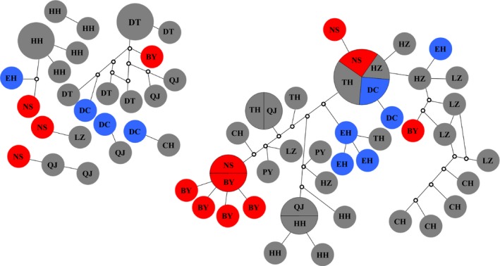
Statistical parsimony haplotype network with a 95 % connection limit for 116 COI sequences (709 bp) of Bellamya aeruginosa constructed with TCS. The size of each circle indicates the frequency of the respective haplotype; unsampled haplotypes are indicated by small empty circles. Red represents haplotypes from the Yellow River system, gray represents haplotypes from the Yangtze River system and blue represents haplotypes from plateau lakes.
Figure 3.

Structure plot for the 12 Bellamya aeruginosa populations based on the microsatellite data (shown for the most likely K = 3). The sampling location codes (Table 1) are indicated along the x‐axis. Each vertical line represents one individual, and y‐coordinates denote each individual's percentage assignment to each of the three genetic clusters.
We found a significant isolation by linear distance pattern for the microsatellite data (Mantel test, r = 0.4888; P = 0.011, Fig. 4A) and COI data (r = 0.5101; P = 0.011, Fig. 4B), when all populations were included. When we only analyzed the populations from the Yangtze catchment, no isolation by linear or stream distance was detected for either data set (Fig. 4C–F).
Figure 4.

Isolation by linear distance across all populations for (A) microsatellite data, and (B) mitochondrial data, and only for the Yangtze River for (C) microsatellite data, and (D) mitochondrial data; isolation by stream distance for the Yangtze River using (E) microsatellite data and (F) mitochondrial data.
Gene flow
Gene flow estimates based on the microsatellite data calculated with MIGRATE and BAYESASS indicated moderate to high levels of gene flow between populations (Tables 4 and 5). MIGRATE estimated the effective number of migrants entering and leaving each population per generation (M) between 1.29 (QJ→DT) and 74.76 (LZ→QJ) (Table 4). Most of populations had asymmetrical gene flow except for HZ, NS, and DC populations. The highest unidirectional estimates of gene flow estimated by MIGRATE were found toward the HH population (M = 188.47) and the lowest was for CH (M = 90.03), while the highest gene flow out of a population was from LZ (M = 251.94). Similarly, many migration rate estimates from BAYESASS were moderate to high, ranging from 0.01 to 0.237 (76 of 144 values); the remainder varied from 0.008 to 0.009 (Table 5).
Table 4.
Immigration rates (M) into each of the 12 Bellamya aeruginosa populations from every other population as estimated by MIGRATE
| pop | CH | DT | PY | QJ | HZ | NS | BY | TH | LZ | HH | EH | DC | Total→i | |
|---|---|---|---|---|---|---|---|---|---|---|---|---|---|---|
| i | Θi | CH→i | DT→i | PY→i | QJ→i | HZ→i | NS→i | BY→i | TH→i | LZ→i | HH→i | EH→i | DC→i | |
| CH | 0.0941 | 7.16 | 3.69 | 9.56 | 6.41 | 6.33 | 9.68 | 19.38 | 3.49 | 4.29 | 15.55 | 4.50 | 90.03 | |
| DT | 0.0953 | 13.95 | 10.70 | 1.29 | 16.00 | 3.57 | 4.75 | 17.56 | 18.04 | 17.68 | 10.20 | 8.17 | 107.97 | |
| PY | 0.0662 | 11.88 | 5.44 | 5.71 | 7.41 | 3.78 | 11.16 | 6.81 | 29.65 | 9.46 | 10.23 | 4.93 | 94.57 | |
| QJ | 0.0468 | 11.37 | 10.59 | 9.45 | 8.43 | 19.77 | 5.12 | 6.84 | 74.76 | 17.13 | 13.08 | 12.45 | 177.61 | |
| HZ | 0.0827 | 35.47 | 7.44 | 18.47 | 1.48 | 10.59 | 25.02 | 13.05 | 8.93 | 13.43 | 7.72 | 8.33 | 114.46 | |
| NS | 0.0920 | 9.59 | 4.99 | 15.03 | 2.41 | 5.55 | 30.59 | 4.46 | 27.47 | 8.43 | 19.06 | 13.58 | 131.56 | |
| BY | 0.0949 | 11.79 | 6.29 | 13.58 | 12.07 | 7.29 | 13.45 | 5.90 | 16.45 | 5.35 | 13.48 | 11.18 | 105.04 | |
| TH | 0.0958 | 12.83 | 12.05 | 35.68 | 19.12 | 16.51 | 13.23 | 7.30 | 4.22 | 8.06 | 7.90 | 2.07 | 126.12 | |
| LZ | 0.0608 | 8.71 | 3.51 | 14.32 | 6.68 | 13.73 | 9.41 | 4.48 | 11.84 | 9.03 | 17.22 | 12.57 | 102.78 | |
| HH | 0.0947 | 10.38 | 17.19 | 21.74 | 7.26 | 11.96 | 10.62 | 20.21 | 15.06 | 54.26 | 11.80 | 18.38 | 188.47 | |
| EH | 0.0855 | 39.47 | 8.07 | 28.56 | 10.82 | 11.84 | 19.84 | 20.18 | 51.26 | 9.98 | 12.84 | 6.18 | 179.55 | |
| DC | 0.0261 | 7.20 | 10.76 | 16.69 | 5.16 | 5.90 | 11.78 | 8.17 | 15.62 | 4.70 | 12.78 | 6.83 | 98.39 | |
| Total | 172.63 | 93.49 | 187.92 | 81.54 | 111.03 | 122.35 | 146.65 | 167.78 | 251.94 | 118.48 | 133.06 | 102.34 | ||
Table 5.
Estimates of migration rates (proportion of individuals) among populations of B. aeruginosa, derived by BAYESASS
| Migration from | |||||||||||||
|---|---|---|---|---|---|---|---|---|---|---|---|---|---|
| BY | NS | HZ | TH | CH | PY | LZ | DT | HH | QJ | DC | EH | ||
| Migration into | BY | 0.678 (0.657–0.698) | 0.225 (0.173–0.277) | 0.009 (0.000–0.026) | 0.009 (0.000–0.027) | 0.009 (0.000–0.026) | 0.009 (0.000–0.026) | 0.017 (0.000–0.041) | 0.009 (0.000–0.026) | 0.009 (0.000–0.026) | 0.009 (0.000–0.026) | 0.009 (0.000–0.026) | 0.009 (0.000–0.026) |
| NS | 0.009 (0.000–0.027) | 0.890 (0.837–0.944) | 0.009 (0.000–0.027) | 0.011 (0.000–0.032) | 0.010 (0.000–0.030) | 0.009 (0.000–0.0.27) | 0.012 (0.000–0.032) | 0.009 (0.000–0.027) | 0.009 (0.000–0.027) | 0.009 (0.000–0.027) | 0.010 (0.000–0.030) | 0.010 (0.000–0.030) | |
| HZ | 0.009 (0.000–0.027) | 0.009 (0.000–0.027) | 0.678 (0.657–0.699) | 0.212 (0.153–0.271) | 0.019 (0.000–0.050) | 0.009 (0.000–0.026) | 0.010 (0.000–0.029) | 0.010 (0.000–0.028) | 0.009 (0.000–0.026) | 0.009 (0.000–0.027) | 0.010 (0.000–0.029) | 0.015 (0.000–0.039) | |
| TH | 0.010 (0.000–0.029) | 0.021 (0.000–0.058) | 0.010 (0.000–0.028) | 0.846 (0.0779–0.913) | 0.019 (0.000–0.052) | 0.010 (0.000–0.028) | 0.015 (0.000–0.044) | 0.012 (0.000–0.035) | 0.010 (0.000–0.028) | 0.010 (0.000–0.029) | 0.020 (0.000–0.053) | 0.018 (0.000–0.050) | |
| CH | 0.008 (0.000–0.024) | 0.008 (0.000–0.024) | 0.008 (0.000–0.023) | 0.044 (0.000–0.093) | 0.857 (0.0797–0.916) | 0.008 (0.000–0.024) | 0.012 (0.000–0.033) | 0.012 (0.000–0.034) | 0.008 (0.000–0.023) | 0.008 (0.000–0.023) | 0.015 (0.000–0.038) | 0.012 (0.000–0.034) | |
| PY | 0.008 (0.000–0.023) | 0.009 (0.000–0.025) | 0.008 (0.000–0.023) | 0.237 (0.189–0.285) | 0.009 (0.000–0.026) | 0.676 (0.658–0.694) | 0.010 (0.000–0.030) | 0.008 (0.000–0.024) | 0.008 (0.000–0.024) | 0.008 (0.000–0.024) | 0.009 (0.000–0.026) | 0.009 (0.000–0.025) | |
| LZ | 0.009 (0.000–0.026) | 0.009 (0.000–0.027) | 0.009 (0.000–0.026) | 0.051 (0.000–0.115) | 0.016 (0.000–0.045) | 0.009 (0.000–0.026) | 0.833 (0.754–0.912) | 0.018 (0.000–0.047) | 0.009 (0.000–0.027) | 0.009 (0.000–0.026) | 0.009 (0.000–0.027) | 0.018 (0.000–0.047) | |
| DT | 0.009 (0.000–0.027) | 0.012 (0.0000–0.033) | 0.010 (0.000–0.028) | 0.034 (0.000–0.00.89) | 0.015 (0.000–0.040) | 0.010 (0.000–0.028) | 0.021 (0.000–0.052) | 0.851 (0.783–0.920) | 0.009 (0.000–0.027) | 0.010 (0.000–0.028) | 0.011 (0.000–0.031) | 0.010 (0.000–0.028) | |
| HH | 0.009 (0.000–0.026) | 0.010 (0.000–0.027) | 0.009 (0.000–0.027) | 0.046 (0.000–0.099) | 0.010 (0.000–0.029) | 0.010 (0.000–0.028) | 0.009 (0.000–0.028) | 0.191 (0.125–0.258) | 0.678 (0.657–0.689) | 0.009 (0.000–0.026) | 0.010 (0.000–0.270) | 0.010 (0.000–0.028) | |
| QJ | 0.008 (0.000–0.024) | 0.009 (0.000–0.025) | 0.008 (0.000–0.025) | 0.198 (0.130–0.027) | 0.008 (0.000–0.024) | 0.008 (0.000–0.024) | 0.046 (0.000–0.104) | 0.012 (0.000–0.033) | 0.008 (0.000–0.024) | 0.677 (0.658–0.695) | 0.008 (0.000–0.024) | 0.009 (0.000–0.025) | |
| DC | 0.011 (0.000–0.031) | 0.015 (0.000–0.042) | 0.011 (0.000–0.031) | 0.014 (0.000–0.039) | 0.018 (0.000–0.047) | 0.011 (0.000–0.030) | 0.014 (0.000–0.0039) | 0.011 (0.000–0.031) | 0.011 (0.000–0.031) | 0.011 (0.000–0.031) | 0.865 (0.805–0.925) | 0.011 (0.000–0.033) | |
| EH | 0.010 (0.000–0.028) | 0.013 (0.000–0.036) | 0.010 (0.000–0.028) | 0.027 (0.000–0.072) | 0.012 (0.000–0.034) | 0.010 (0.000–0.028) | 0.012 (0.000–0.033) | 0.010 (0.000–0.030) | 0.010 (0.000–0.029) | 0.010 (0.000–0.029) | 0.015 (0.000–0.043) | 0.863 (0.795–0.863) | |
Means of the posterior distributions of m, the migration rate into each population, are shown. The populations from which each individual was sampled are listed in the rows, while their populations from which they migrated are listed in the columns. Values along the diagonal are the proportions of individuals derived from the source populations each generation. Values in parentheses below migration rates are 95% CI.
Current and historical demography
The effective population size estimates derived from LDN e analyses were not very precise, appeared to vary between populations, yet were mostly large (estimated as infinite for five of the 12 populations, range of other populations from 55 for CH to 1006 for YX).
BOTTLENECK analyses of the microsatellite data revealed no evidence of a recent bottleneck for most of populations except for the HH and QJ populations. No significant heterozygosity excess was detected in any locality under the TPM.
The Bayesian skyline plots detected relatively stable population sizes throughout the last 2 mya for most populations (Fig. 5). The overall population size of the species in the study region appears to have increased constantly from 3 mya to 300 kya, when the population sizes strongly dropped. Subsequent to this drop, population size recovered quickly even extending predecline population size.
Figure 5.

BSP (Bayesian Skyline Plots) generated using the cytochrome oxidase I sequences and applying a fixed mutation rate of 1.34% sequence divergence per million years and the HKY + I + G model as determined by jModeltest. BSPs were generated for (A) each population and (B) for the species as a whole. Red – Yellow River, gray – Yangtze River, blue – plateau lakes. Dotted line – all populations combined , grey dotted line – 95 % HPD.
Discussion
Our population genetic analysis of B. aeruginosa supports our first scenario: we found high levels of genetic diversity and strong population admixture across the 12 studied populations of B. aeruginosa for both mitochondrial and nuclear markers despite a sessile life style and large separating geographic distances. Current population sizes appear to be mostly large, which was also supported by the high genetic diversity and past fluctuations of population sizes appear to be limited. However, the species as a whole seems to have rapidly declined during the mid‐ to Late Pleistocene and postglacially expanded. Yet, no recent bottlenecks were detected with the microsatellite data. Our findings suggest that gene flow is moderate to high among the sampling locations, even between river systems despite vast geographic distances and low active dispersal ability. The results further indicate that the species at the moment can maintain high genetic diversity despite strong harvesting pressure and increasing fragmentation. These findings may be explained by a combination of large population sizes with high standing genetic variation and long‐distance gene flow, potentially facilitated by zoochoric and anthropogenic dispersal. In the following, we discuss each of these findings in detail.
Genetic diversity and current and past population demography
Both marker systems revealed high genetic diversity and low levels of genetic differentiation between local populations (Tables 1, 2, 3, 4, Figs. 2, 3). Current population sizes were generally large and confidence intervals in all, but one population included infinity. Population sizes of single populations appeared to be relatively stable with increases or declines occurring within the last 500 ka, independent of the stream system (Fig. 5). Overall, the population size of all combined populations constantly increased starting 3 mya with a sudden drop around 300 kya. Within the last 100 ka, the population sizes increased again even exceeding the predecline size (Fig. 5).
Our findings suggest that the demographic history of the species has been influenced by past climatic cycles with a drop in population size corresponding to the Late Pleistocene and postglacial range expansion (Yang et al. 2009; Bagley et al. 2013). For ten populations, we detected a drop in population size from mid‐ or Late Pleistocene (Fig. 5). The Tali glacial stage of the Late Pleistocene (10–110 ka) likely had a great influence on the distribution of Bellamya in plateau lakes, while the Taku glaciation in the early Mid‐Pleistocene and the Lushan glaciation in the Late Mid‐Pleistocene (200–230 ka) (Wissmann 1937; Tang and Tao 1997; Xiang et al. 2006) may have led to a fast decline of Bellamya populations across the Yangtze River system. At more recent time scales, microsatellites could not detect bottlenecks for most populations suggesting no recent drastic population declines. The current population sizes are likely large and together with high migration rates allow for the maintenance of high genetic diversity. These findings of high genetic diversity and little differentiation is comparatively uncommon in freshwater snails in lakes due to their low migration ability, high self‐fertilization rates, and historical demographic instability (Campbell et al. 2010; Nalugwa et al. 2011; Standley et al. 2014). However, Bellamya is somewhat special as the genus has a relatively short generation time of only 4 months (Ma et al. 2010), which in combination with their specific mating strategy (gonochorism and viviparity), may make them less vulnerable to rapid loss of genetic diversity resulting from population fluctuations and geographic isolation (Li et al. 2011; Tian‐Bi et al. 2013). Further, the lacustrine habitats may represent relatively stable habitats, which allow for large stable population sizes, further helping to maintain high genetic diversity. Hence, the combination of the environmental setting and species specific life‐history traits together promotes the maintenance of large stable populations in B. aeruginosa.
Low population divergence and weak geographic structure
Another aspect potentially contributing to the high genetic diversity are high migration rates, even between far distant populations. We found that the study populations are only slightly differentiated from each other. F ST and ΦST values were low and mostly insignificant. We found a significant signal of isolation by distance for both genetic markers across the whole study region (Fig. 4A and B). Isolation by distance and isolation by stream distance in the Yangtze River, however, were much weaker (Fig. 4C–F). AMOVA showed limited divergence between populations and regions for both data sets (Tables 2). Bayesian inference of recent migration rates suggested consistent, intermediate to high levels level of gene flow between populations (Table 5). The haplotype network for the mitochondrial data showed little sorting of locations (Fig. 2) and STRUCTURE suggested three lineages; yet, these only partially correspond to the stream systems and geographic regions.
All these findings together suggest that gene flow is moderate to high and not only occurs within streams, but also between different drainages (Yangtze River and Yellow River); even isolated plateau lakes receive migrants. Within the Yangtze River for which we have the largest number of samples, no strong isolation by stream distance was detected, suggesting that populations along the stream frequently exchange individuals. The absence of significant isolation by distance and weak geographic signal among populations is not uncommon in snail species (Wada et al. 2012). This may at least in riverine systems partially be due to frequent flooding events during which specimens may be swept away and transported even to far distant locations within the stream (Van Leeuwen et al. 2013). Accidental transport during flooding may change population genetic patterns within rivers and even completely remove isolation by distance patterns (Crispo and Chapman 2009). Such flash floods are common in the Yangtze River catchment, and all of the lakes sampled in this catchment are connected to the river.
Flooding, however, cannot explain the strong admixture between far distant sampling locations across different river systems and isolated plateau lakes (as seen e.g., in Figs. 2, 3). Here, anthropogenic translocations and animal‐mediated dispersal via waterfowl represent a possible explanation, a commonly observed phenomenon in freshwater snails (Green and Figuerola 2005; Gittenberger et al. 2006; Gittenberger 2012; Kopp et al. 2012). Human‐ and animal‐mediated dispersal, for example, explains the present day distribution of Isabellaria buresi pharsalica in Thessaly (Uit de Weerd et al. 2005). As Bellamya are commonly harvested by humans, anthropogenic translocations appear likely for this genus (Prabhakar and Roy 2009; Li et al. 2010). Such translocations, independent of the vector, appear to have positive effects on the genetic diversity of the species.
Conclusion
Our genetic analysis revealed high levels of intrapopulation genetic variation, large effective population sizes, moderate to high levels of gene flow, and low interpopulation differentiation. The high rates of gene flow within the Yangtze catchment may be supported by drifting during frequent flooding events, while gene flow between different catchments likely is facilitated by animal‐ or human‐mediated dispersal. All together, the conservation status of the species seems currently uncritical despite strong harvesting pressure and anthropogenic habitat fragmentation.
Conflict of Interest
None declared.
Supporting information
Figure S1. Distributions of pairwise nucleotide differences (mismatch distributions) of COI gene in B. aeruginosa samples and the corresponding Fu's Fs value.
Figure S2. The most likely value of K (inferred cluster) estimated using Evanno's ΔK‐method.
Table S1. Primer sequence for microsatellite markers and optional PCR conditions.
Table S2. The frequencies of null alleles across seven microsatellite loci and 12 geographic locations for B. aeruginosa, as suggested by the program MICRO‐CHECKER.
Acknowledgments
This work was financially supported by the National Natural Science Foundation of China (No. 31172410). We thank Jesse W. Ray for help with calculations of stream distances in Figure 1.
Ecology and Evolution 2015; 5(21): 4906–4919
References
- Bagley, J. C. , Sandel M., Travis J., de Lourdes Lozano‐Vilano M., and Johnson J. B.. 2013. Paleoclimatic modeling and phylogeography of least killifish, Heterandria formosa: insights into Pleistocene expansion‐contraction dynamics and evolutionary history of North American Coastal Plain freshwater biota. BMC Evol. Biol. 13:223. doi:10.1186/1471‐2148‐13‐223. [DOI] [PMC free article] [PubMed] [Google Scholar]
- Beerli, P. , and Felsenstein J.. 2001. Maximum likelihood estimation of a migration matrix and effective population sizes in n subpopulations by using a coalescent approach. Proc. Natl Acad. Sci. USA 98:4563–4568. [DOI] [PMC free article] [PubMed] [Google Scholar]
- Bohonak, A. J. 2002. IBD (isolation by distance): a program for analyses of isolation by distance. J. Hered. 93:153–154. [DOI] [PubMed] [Google Scholar]
- Bürgmann, H. , Pesaro M., Widmer F., and Zeyer J.. 2001. A strategy for optimizing quality and quantity of DNA extracted from soil. J. Microbiol. Methods 45:7–20. [DOI] [PubMed] [Google Scholar]
- Campbell, G. , Noble L. R., Rollinson D., Southgate V. R., Webster J. P., and Jones C. S.. 2010. Low genetic diversity in a snail intermediate host (Biomphalaria pfeifferi Krass, 1848) and schistosomiasis transmission in the Senegal River Basin. Mol. Ecol. 19:241–256. [DOI] [PubMed] [Google Scholar]
- Chaine, N. M. , Allen C. R., Fricke K. A., Haak D. M., Hellman M. L., Kill R. A., et al. 2012. Population estimate of Chinese mystery snail (Bellamya chinensis) in a Nebraska reservoir. Bioinv. Rec. 1:283–287. [Google Scholar]
- Clement, M. , Posada D., and Crandall K. A.. 2000. TCS: a computer program to estimate gene genealogies. Mol. Ecol. 9:1657–1660. [DOI] [PubMed] [Google Scholar]
- Crispo, E. , and Chapman L. J.. 2009. Temporal variation in population genetic structure of a Riverine African cichlid fish. J. Hered. 101:97–106. [DOI] [PubMed] [Google Scholar]
- Darriba, D. , Taboada G. L., Doallo R., and Posada D.. 2012. jModelTest 2: more models, new heuristics and parallel computing. Nat. Methods 9:772. [DOI] [PMC free article] [PubMed] [Google Scholar]
- Dieringer, D. , and Schlötterer C.. 2003. MICROSATELLITE ANALYZER (MSA): a platform independent analysis tool for large microsatellite data sets. Mol. Ecol. Notes 3:167–169. [Google Scholar]
- Do, C. , Waples R. S., Peel D., Macbeth G. M., Tillett B. J., and Ovenden J. R.. 2014. NeEstimator v2.0: re‐implementation of software for the estimation of contemporary effective population size (N e) from genetic data. Mol. Ecol. Resour. 41:209–214. [DOI] [PubMed] [Google Scholar]
- Drummond, A. J. , Suchard M. A., Xie D., and Rambaut A.. 2012. Bayesian phylogenetics with BEAUti and the BEAST 1.7. Mol. Biol. Evol. 29:1969–1973. [DOI] [PMC free article] [PubMed] [Google Scholar]
- Eberhart‐Phillips, L. J. , Hoffman J. I., Brede E. G., Zefania S., Kamrad M. J., Székely T., et al. 2015. Contrasting genetic diversity and population structure among three sympatric Madagascan shorebirds: parallels with rarity, endemism, and dispersal. Ecol. Evol. 5:997–1010. [DOI] [PMC free article] [PubMed] [Google Scholar]
- Epps, C. W. J. D. , Roderick G. K., Ramey R. B., and McCullough D. R.. 2005. Highways block gene flow and cause a rapid decline in genetic diversity of desert bighorn sheep. Ecol. Lett. 8:1029–1038. [Google Scholar]
- ESRI . 2011. ArcGIS Desktop: Release 10. Environmental Systems Research Institute, Redlands, CA. [Google Scholar]
- Evanno, G. , Regnaut S., and Goudet J.. 2005. Detecting the number of clusters of individuals using the software STRUCTURE: a simulation study. Mol. Ecol. 14:2611–2620. [DOI] [PubMed] [Google Scholar]
- Excoffier, L. , and Lischer H. L.. 2010. 3.5: a new series of programs to perform population genetics analyses under Linux and Windows. Mol. Ecol. Resour. 10:564–567. [DOI] [PubMed] [Google Scholar]
- Faubet, P. , Waples R. S., and Gaggiotti O. E.. 2007. Evaluating the performance of a multilocus bayesian method for the estimation of migration rates. Mol. Ecol. 16:1149–1166. [DOI] [PubMed] [Google Scholar]
- Fernández‐García, J. L. , Carranza J., Martínez J. G., and Randi E.. 2014. Mitochondrial D‐loop phylogeny signals two native Iberian red deer (Cervus elaphus) Lineages genetically different to Western and Eastern European red deer and infers human‐mediated translocations. Biodiv. Conserv. 23:537–554. [Google Scholar]
- Folmer, O. , Black M., Hoeh W., Lutz R., and Vrijenhoek R.. 1994. DNA primers for amplification of mitochondrial cytochrome c oxidase subunit I from diverse metazoan invertebrates. Mol. Mar. Biol. Biotechnol 3:294–299. [PubMed] [Google Scholar]
- Fu, Y. X. 1997. Statistical tests of neutrality of mutations against population growth, hitchhiking and background selection. Genetics 147:915–925. [DOI] [PMC free article] [PubMed] [Google Scholar]
- Gittenberger, E. 2012. Long‐distance dispersal of molluscs: ‘Their distribution at first perplexed me much’. J. Biogeogr. 39:10–11. [Google Scholar]
- Gittenberger, E. , Groenenberg D. S. J., Kokshoorn B., and Preece R. C.. 2006. Biogeography: molecular trails from hitch‐hiking snails. Nature 439:409. [DOI] [PubMed] [Google Scholar]
- González‐Astorga, J. , and Núñez‐Farfán J.. 2001. Effect of habitat fragmentation on the genetic structure of the narrow endemic Brongniartia vazquezii . Evol. Ecol. Res. 3:861–872. [Google Scholar]
- Green, A. J. , and Figuerola J.. 2005. Recent advances in the study of long‐distance dispersal of aquatic invertebrates via birds. Divers. Distrib. 11:149–156. [Google Scholar]
- Harrison, R. G. 1991. Molecular changes at speciation. Annu. Rev. Ecol. Syst. 22:281–308. [Google Scholar]
- Hurtrez‐Boussès, S. , Hurtrez J. E., Turpin H., Durand C., Durand P., De Meeüs T., et al. 2010. Hydrographic network structure and population genetic differentiation in a vector of fasciolosis, Galba truncatula . Infect Genet. Evol. 10:178–183. [DOI] [PubMed] [Google Scholar]
- Husemann, M. , Ray J. W., King R. S., Hooser E. A., and Danley P.. 2012. Comparative biogeography reveals differences in population genetic structure of five species of stream fishes. Biol. J. Linn. Soc. 107:867–885. [Google Scholar]
- Jakobsson, M. , and Rosenberg N. A.. 2007. CLUMPP: a cluster matching and permutation program for dealing with label switching and multimodality in analysis of population structure. Bioinformatics 23:1801–1806. [DOI] [PubMed] [Google Scholar]
- Kopp, K. C. , Wolff K., and Jokela J.. 2012. Natural range expansion and human‐assisted introduction leave different genetic signatures in a hermaphroditic freshwater snail. Ecol. Evol. 26:483–498. [Google Scholar]
- Li, X. Y. , Li Y., Zhou S. Q., and Yan B. L.. 2010. Analysis and evaluation of nutritional composition in two freshwater fingersnails. Food Sci. 31:276–279. [Google Scholar]
- Li, D. L. , Zhang T., Yu J. B., Mao X. W., Wang H. Q., Chen K. J., et al. 2011. Temporal and spatial distribution patterns of mollusca in a typical Aquacultural LAKE—Datong Lake. Acta Hydrobiol. Sin. 35:946–954. [Google Scholar]
- Librado, P. , and Rozas J.. 2009. DnaSP v5: a software for comprehensive analysis of DNA polymorphism data. Bioinformatics 25:1451–1452. [DOI] [PubMed] [Google Scholar]
- Ma, T. , Gong S., Zhou K., Zhu C., Deng K., Luo Q., et al. 2010. Laboratory culture of the freshwater benthic gastropod Bellamya aeruginosa (Reeve) and its utility as a test species for sediment toxicity. J. Environ. Sci. 22:304–313. [DOI] [PubMed] [Google Scholar]
- Meirmans, P. G. 2014. Nonconvergence in bayesian estimation of migration rates. Mol. Ecol. Res. 14:726–733. [DOI] [PubMed] [Google Scholar]
- Nalugwa, A. , Jørgensen A., Nyakaana S., and Kristensen T. K.. 2011. Genetic variation within and between populations of hermaphroditic Bulinus truncatus tetraploid freshwater snails of the Albertine Rift, East Africa. Hydrobiologia 673:53–61. [Google Scholar]
- Nekola, J. C. 2012. The impact of a utility corridor on terrestrial gastropod biodiversity. Biodiv. Conserv. 21:781–795. [Google Scholar]
- Nilsson, C. , Reidy C. A., Dynesius M., and Revenga C.. 2005. Fragmentation and flow regulation of the world's large river systems. Science 308:405–408. [DOI] [PubMed] [Google Scholar]
- Ozawa, K. , Yokoyama A., Ishikawa K., Kumagai M., Watanabe M. F., and Park H. D.. 2003. Accumulation and depuration of microcystin produced by the cyanobacterium Microcystis in a freshwater snail. Limnology 4:131–138. [Google Scholar]
- Piry, S. , Luikart G., and Cornuet J. M.. 1999. BOTTLENECK: a computer program for detecting recent reductions in the effective population size using allele frequency data. J. Hered. 90:502–503. [Google Scholar]
- Prabhakar, A. K. , and Roy S. P.. 2009. Ethno‐medicinal uses of some shell fishes by people of Kosi river basin of North‐Bihar, India. Ethno‐Med. 3:1–4. [Google Scholar]
- Pritchard, J. K. , Stephens M., and Donnelly P.. 2000. Inference of population structure using multilocus genotype data. Genetics 155:945–959. [DOI] [PMC free article] [PubMed] [Google Scholar]
- R Development Core Team . 2009. R: a language and environment for statistical computing. R Foundation for Statistical Computing, Vienna, Austria. [Google Scholar]
- Ray, J. W. , Husemann M., Lutz‐Carrillo D. J., King R. S., and Danley P. D.. 2015. Life at the leading edge: genetic impoverishment of the spotted bass, Micropterus punctulatus, at its Western edge. Environmental Biology of Fishes 98:1823‐1832. [Google Scholar]
- Rambaut, A. , and Drummond A. J.. 2009. Tracer 1.5.0. MCMC Trace Analysis Tool. Available at http://beast.bio.ed.ac.uk/Tracer. (accessed 10 April 2014).
- Reed, D. H. , and Frankham R.. 2003. Correlation between fitness and genetic diversity. Conservation Biology 17:230‐237. [Google Scholar]
- Ricciardi, A. , and Rasmussen J. B.. 1999. Extinction rates of North American freshwater fauna. Conserv. Biol. 13:1220–1222. [Google Scholar]
- Rice, W. R. 1989. Analyzing tables of statistical tests. Evolution 43:223–225. [DOI] [PubMed] [Google Scholar]
- Roberts, J. H. , Angermeier P. L., and Hallerman E. M.. 2013. Distance, dams and drift: what structures populations of an endangered, benthic stream fish? Freshwater Biol. 58:2050–2064. [Google Scholar]
- Roffler, G. H. , Talbot S. L., Luikart G., Sage G. K., Pilgrim K. L., Adams L. G., et al. 2014. Lack of sex‐biased dispersal promotes fine‐scale genetic structure in alpine ungulates. Conserv. Genet. 15:837–851. [Google Scholar]
- Rosenberg, N. A. 2004. Distruct: a program for the graphical display of population structure. Mol. Ecol. Notes 4:137–138. [Google Scholar]
- Rousset, F. 2008. Genepop'007: a complete re‐implementation of the Genepop software for Windows and Linux. Mol. Ecol. Res. 8:103–106. [DOI] [PubMed] [Google Scholar]
- Schultheiß, R. , Wilke T., Jørgensen A., and Albrecht C.. 2011. The birth of an endemic species flock: demographic history of the Bellamya group (Gastropoda, Viviparidae) in Lake Malawi. Biol. J. Linn. Soc. 102:130–143. [Google Scholar]
- Sinclair‐Winters, C. M. 2014. Upstream or downstream? Population structure of the land snail Ventridens ligera (Say, 1821) in the Potomac River drainage basin. J. Mollus. Stud. 80:280–285. [Google Scholar]
- Song, L. , Chen W., Peng L., Wan N., Gan N. Q., and Zhang X. M.. 2007. Distribution and bioaccumulation of microcystins in water columns: a systematic investigation into the environmental fate and the risks. associated with microcystins in Meiliang Bay, Lake Taihu. Water Res. 41:2853–2864. [DOI] [PubMed] [Google Scholar]
- Standley, C. J. , Goodacre S. L., Wade C. M., and Stothard J. R.. 2014. The population genetic structure of Biomphalaria choanomphala in Lake Victoria, East Africa: implications for schistosomiasis transmission. Parasite. Vector. 7:524. doi:10.1186/s13071‐014‐0524‐4. [DOI] [PMC free article] [PubMed] [Google Scholar]
- Tang, G. Z. , and Tao M.. 1997. Discussion on relationship between the middle Pleistocene glaciation and formation of the Yangtze Gorges. Geology and Mineral Resources of South China 4:9–18 (in Chinese). [Google Scholar]
- Tajima, F. 1989. Statistical method for testing the neutral mutation hypothesis by DNA polymorphism. Genetics 123:585–595. [DOI] [PMC free article] [PubMed] [Google Scholar]
- Thompson, J. D. , Gibson T. J., Plewniak F., Jeanmougin F., and Higgins D. G.. 1997. The Clustal X windows interface: flexible strategies for multiple sequences alignment aided by quality analysis tools. Nucleic Acids Res. 25:4876–4882. [DOI] [PMC free article] [PubMed] [Google Scholar]
- Tian‐Bi, Y. N. T. , Jarne P., Konan J. N. K., Utzinger J., and N'Goran E. K.. 2013. Contrasting the distribution of phenotypic and molecular variation in the freshwater snail Biomphalaria pfeifferi, the intermediate host of Schistosoma mansoni . Heredity 110:466–474. [DOI] [PMC free article] [PubMed] [Google Scholar]
- Tibbets, C. A. , and Dowling T. E.. 1996. Effects of intrinsic and extrinsic factors on population fragmentation in three species of North American minnows (Teleostei: Cyprinidae). Evolution 50:1280–1292. [DOI] [PubMed] [Google Scholar]
- Toro, M. A. , and Caballero A.. 2005. Characterization and conservation of genetic diversity in subdivided populations. Philos. Trans. R. Soc. Lond. B Biol. Sci. 360:1367–1378. [DOI] [PMC free article] [PubMed] [Google Scholar]
- Uit de Weerd, D. R. , Schneider D., and Gittenberger E.. 2005. The provenance of the Greek land snail species Isabellaria pharsalica: molecular evidence of recent passive long‐distance dispersal. J. Biogeogr. 32:1571–1581. [Google Scholar]
- Van Bocxlaer, B. , and Hunt G.. 2013. Morphological stasis in an ongoing radiation from Lake Malawi. Proc. Natl Acad. Sci. USA 110:13892–13897. [DOI] [PMC free article] [PubMed] [Google Scholar]
- Van Leeuwen, C. H. A. , Huig N., Van der Velde G., Van Alen T. A., Wagemaker C. A. M., Sherman C. D. H., et al. 2013. How did this snail get here? Multiple dispersal vectors inferred for an aquatic invasive species. Freshwater Biol. 58:88–99. [Google Scholar]
- Van Oosterhout, C. , Hutchinson W. F., Wills D. P. M., and Shipley P.. 2004. MICRO‐CHECKER: software for identifying and correcting genotyping errors in microsatellite data. Mol. Ecol. Notes 4:535–538. [Google Scholar]
- Vellend, M. , and Geber M. A.. 2005. Connections between species diversity and genetic diversity. Ecol. Lett. 8:767–781. [Google Scholar]
- Wada, S. , Kawakami K., and Chiba S.. 2012. Snails can survive passage through a bird's digestive system. J. Biogeogr. 39:69–73. [Google Scholar]
- Waples, R. S. , and Gaggiotti O.. 2006. What is a population? An empirical evaluation of some genetic methods for identifying the number of gene pools and their degree of connectivity. Mol. Ecol. 15:1419–1439. [DOI] [PubMed] [Google Scholar]
- Weir, B. S. , and Cockerham C. C.. 1984. Estimating F‐statistics for the analysis of population structure. Evolution 38:1358–1370. [DOI] [PubMed] [Google Scholar]
- Willi, Y. , Van Buskirk J., and Hoffmann A. A.. 2006. Limits to the adaptive potential of small populations. Annual Reviews of Ecology, Evolution and Systematics 37:433‐458. [Google Scholar]
- Wissmann, H. 1937. The Pleistocene glaciation in China. Bulletin of the Geological Society of China 17:145‐168. [Google Scholar]
- Wilke, T. , Schultheiß R., and Albrecht C.. 2009. As time goes by: a simple fool's guide to molecular clock approaches in invertebrates. Am. Malacol. Bull. 27:25–45. [Google Scholar]
- Wilson, G. A. , and Rannala B.. 2003. Bayesian inference of recent migration rates using multilocus genotypes. Genetics 163:1177–1191. [DOI] [PMC free article] [PubMed] [Google Scholar]
- Xiang, B. X. , Xiang Z., and Xiang Y. H.. 2006. Investigation of wild Ginkgo biloba in Wuchuan county of Guizhou, China—Guizhou ancient Ginkgo biloba resources investigation VII. Guizhou Sci. 24:56‐67 (in Chinese with an English abstract). [Google Scholar]
- Yang, L. , Mayden R. L., and He S. P.. 2009. Population genetic structure and geographical differentiation of the Chinese catfish Hemibagrus macropterus (Siluriformes, Bagridae): Evidence for altered drainage patterns. Mol. Phylogenet. Evol. 51:405–411. [DOI] [PubMed] [Google Scholar]
- Zhang, X. , and Liu Y. Y.. 1960. Morphology and habitat of common Bellamya in China. B. Biol. 2:49–57. [Google Scholar]
- Zuberogoitia, I. , Zalewskah H., Zabala J., and Zalewski A.. 2013. The impact of river fragmentation on the population persistence of native and alien mink: an ecological trap for the endangered European mink. Biodivers. Conserv. 22:169–186. [Google Scholar]
Associated Data
This section collects any data citations, data availability statements, or supplementary materials included in this article.
Supplementary Materials
Figure S1. Distributions of pairwise nucleotide differences (mismatch distributions) of COI gene in B. aeruginosa samples and the corresponding Fu's Fs value.
Figure S2. The most likely value of K (inferred cluster) estimated using Evanno's ΔK‐method.
Table S1. Primer sequence for microsatellite markers and optional PCR conditions.
Table S2. The frequencies of null alleles across seven microsatellite loci and 12 geographic locations for B. aeruginosa, as suggested by the program MICRO‐CHECKER.