Abstract
Populations in variable environments are described by both a mean growth rate and a variance of stochastic population growth. Increasing variance will increase the width of confidence bounds around estimates of population size, growth, probability of and time to quasi-extinction. However, traditional sensitivity analyses of stochastic matrix models only consider the sensitivity of the mean growth rate.
We derive an exact method for calculating the sensitivity of the variance in population growth to changes in demographic parameters. Sensitivities of the variance also allow a new sensitivity calculation for the cumulative probability of quasi-extinction. We apply this new analysis tool to an empirical dataset on at-risk polar bears to demonstrate its utility in conservation biology
We find that in many cases a change in life history parameters will increase both the mean and variance of population growth of polar bears. This counterintuitive behaviour of the variance complicates predictions about overall population impacts of management interventions. Sensitivity calculations for cumulative extinction risk factor in changes to both mean and variance, providing a highly useful quantitative tool for conservation management.
The mean stochastic growth rate and its sensitivities do not fully describe the dynamics of population growth. The use of variance sensitivities gives a more complete understanding of population dynamics and facilitates the calculation of new sensitivities for extinction processes.
Keywords: conservation, extinction, polar bears, population growth, population viability, sensitivity, stochastic matrix model, variance of population growth
Introduction
All natural populations experience some random environmental variation. Mounting evidence suggests that the frequency and severity of environmental variation is changing, at local and global scales. Consequently, stochastic modeling approaches have become increasingly common in conservation studies concerned with predicting population persistence (Lande et al., 2003; Morris and Doak, 2002; Boyce et al., 2006). Environmental variation is also important when studying life history evolution, where the degree of variation is expected to contribute to the evolution of lifespan and reproductive traits (Morris et al., 2008; Tuljapurkar and Horvitz, 2006).
Stochastic matrix models have become a standard tool for investigating population growth in variable environments. These models describe populations in terms of temporally and/or spatially variable vital rates that quantify transition rates between stages that may be age classes, ontogenetic stages, spatial regions, or other characteristics. The long-run growth rate of such a population is the stochastic growth rate a. This growth rate is widely used in biology as a fitness measure in evolutionary problems(see Tuljapurkar et al. (2009) for a discussion), and as a descriptor of growth or persistence in ecological and PVA analyses (eg. Morris and Doak (2002)).
As important as the growth rate itself is its sensitivity to changes in model parameters. Deterministic sensitivities measure the effect on growth rate of a small change in one or several matrix elements, assuming all other rates remain constant (ie, its derivative) (Caswell, 2001). These changes are called perturbations, and they can be chosen to evaluate sensitivities with distinct biological meanings. (One can measure sensitivity to changing a single vital rate, or to changing all of them, for example.) A closely related quantity, elasticity, measures the proportional response of growth rate to proportional, rather than absolute, perturbations. Tuljapurkar (1990) found an exact method for calculating sensitivities of the stochastic growth rate. Tuljapurkar and Horvitz (Tuljapurkar et al., 2003) demonstrated how to decompose the proportional sensitivity of the growth rate into changes in the means and to changes in the variances of life history parameters. It is also possible to assess sensitivity and elasticity to perturbations within a single environment or subset of environments within an overall range of specified environmental states (Aberg et al., 2009; Ezard et al., 2008; Caswell, 2005). Habitat-specific sensitivities can be important for populations experiencing frequent disturbance, or when environmental variation is defined by specific variables like rainfall or temperature. In the stochastic case, one can estimate stochastic sensitivities using Tuljapurkar’s approximation (Tuljapurkar, 1982) if environmental variation is small (see Caswell, 2001 for an exposition).
However, in stochastic environments both a mean growth rate and a variance are required to fully describe population dynamics (Tuljapurkar and Orzack, 1980). Consider a population composed of N individuals at time t. Define the total population growth over time t as Λ(t) = N(t)/N(0). In the limit of large t, log Λ(t) is asymptotically normally distributed (Tuljapurkar and Orzack, 1980). Suppose we have many sample paths of the stochastic environmental process, then for large t we can estimate the mean stochastic growth rate as â = log Λ(t)/t and its variance across sample paths as υ̂ = Var[log Λ(t)]/t. This variance (υ) is used in studying population extinction (Beissinger and McCullough, 2002), analyzing time series of population data (Lande et al., 2006; Saether et al., 2007; Engen et al., 2005), estimation of effective population size (Engen et al., 2010), and making stochastic population forecasts (Lee and Tuljapurkar, 1994). For a complete picture of stochastic population dynamics we need to understand the properties of υ, not just of a. Particularly in situations where υ is large, a distribution-focused approach may be more appropriate than existing mean-focused sensitivity analyses.
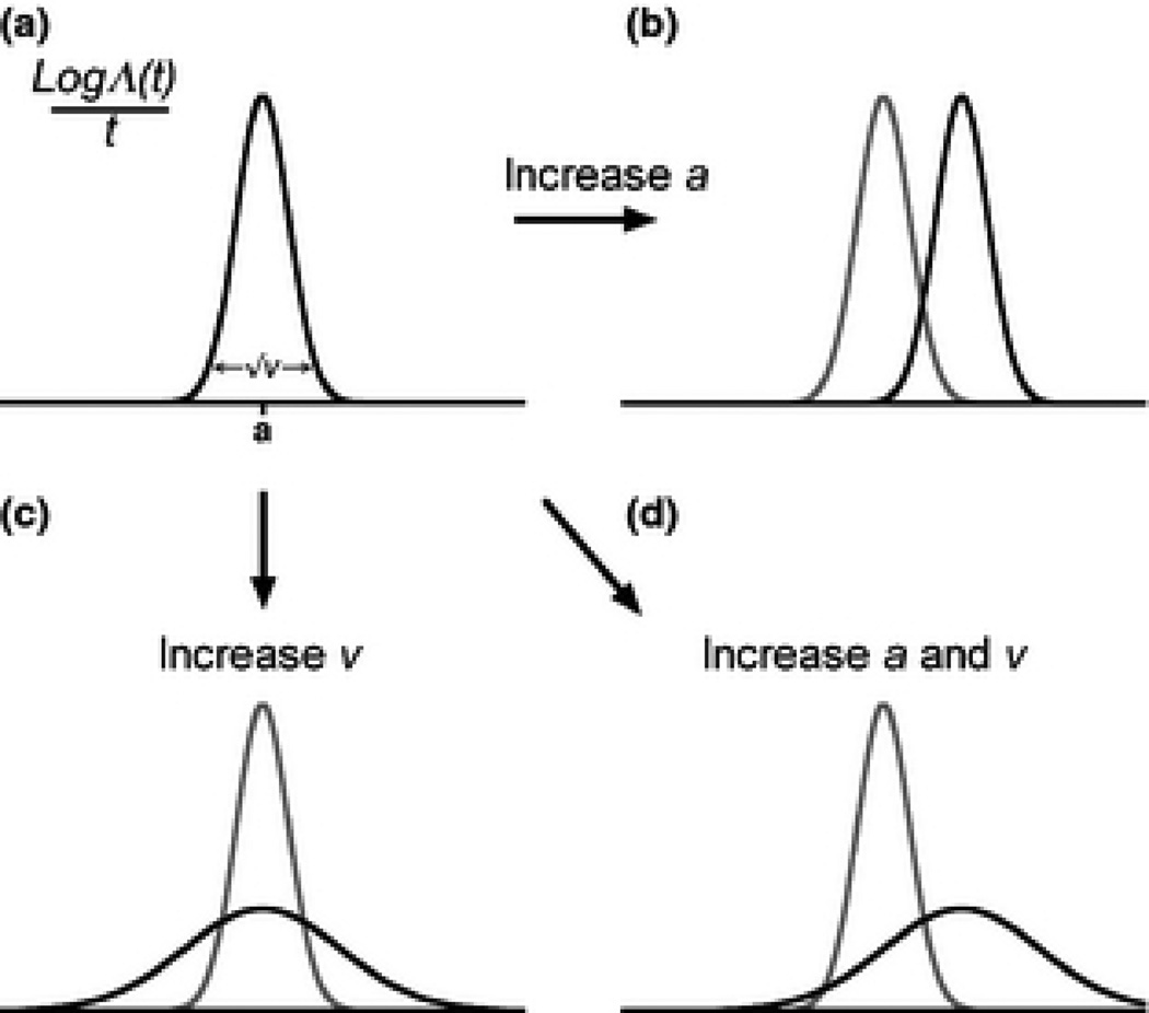
As illustrated in Figure 1, there are several ways the distribution of population growth could respond to perturbation (Tuljapurkar and Orzack, 1980). We aim to examine two questions : 1) how does one formulate a joint-interpretation of sensitivities of the distribution of population growth that accounts for changes to both the mean and the variance? 2) Under what circumstances is it appropriate to use only a mean-focused sensitivity analysis, and when should biologists use our more distribution-focused framework?
Figure 1.
A schematic illustration of the different effects of changing the mean versus the variance of a distribution. A: An example distribution of . In the limit of large t, the mean of this distribution converges on a, and the variance to υ. B: Distribution A after changing only the mean C: Distribution A after changing only the variance D: Distribution A after an increase to both mean and variance
Here we present a new exact method for calculating the sensitivity of the variance of stochastic population growth (υ). Our formulas apply to general kinds of stochastic variation (large or small, serially correlated or not) in models with a general age-stage structure. The general sensitivity calculation allows us to estimate sensitivities and elasticities of the variance to specific changes in life history parameters both across habitats and in specific habitat states. The variance sensitivity also allows the calculation of the sensitivity of cumulative extinction risk, which is useful in studying conservation.
We apply the new sensitivity calculations to empirical data from an at-risk population of polar bears (Ursus Maritimus) (Hunter et al., 2007, 2010) and discuss the results in the context of conservation management. Increases in stochastic variation necessarily increase the uncertainty of population projections and decrease predicted persistence times. It is clear that management efforts will benefit in several ways from an understanding of which vital rates most strongly affect υ. We are especially interested in cases where a and υ respond differently to the same change in a particular vital rate. Our results raise important questions about how we should interpret a change that increases both the mean and the variance of growth. Can we manage for both a and υ?
Materials and Methods
Structure and Assumptions of the Population Model
We work with discrete time matrix population models. (The work of Ellner and Rees (2006) shows that our results will also apply to integral population models (IPMs).) We suppose that individuals are in discrete stages that may be age classes, stage classes (e.g., Caswell (2001)), age-stage classes (e.g., (Lebreton, 1996), or spatial habitats. Newborns constitute stage 1 (but our results extend to cases with additional modes of reproduction such as clonal or vegetative reproduction). The population is counted at discrete intervals and there are per-capita rates x(c, d, t) at which an individual in stage d at t contributes individuals to stage c at time t + 1. These vital rates include sexual reproduction, survival, growth, reversion, migration and so on. At time t the population projection matrix is X(t) with elements x(c, d, t). Population numbers are contained in a vector with components n(c, t) and total population is P(t). There is a known initial population vector N(0) and population changes over time according to
Temporal variation in vital rates is driven by changing environmental conditions. Environments are assumed to change according to a stochastic process that is ergodic and mixing. Such processes include (a) choosing environments from the same probability distribution independently in each time period, (b) using a linear stable time series model for the environmental driver, (c) choosing environments from an ergodic (irreducible and aperiodic) Markov chain with k states. At each t the state of the environment determines the matrix of vital rates. We assume that the set of population projection matrices obey the conditions for demographic weak ergodicity (Cohen, 1979; Lange and Holmes, 1981).
Let X(t) be a (time-varying) random matrix that obeys these assumptions. After a period of T years the population’s dynamics depend on a product of population projection matrices X(T)X(T − 1)…X(1). Over this interval the cumulative growth of population number is, say, Λ(T). Suppose we have many independent sample paths of this process, each of length T time steps. The stochastic growth rate of the population is the same for each sample path, j:
| (1) |
where 𝔼 indicates the expectation over all environments. The variance of stochastic growth is computed across sample paths, and grows at a rate:
| (2) |
Tuljapurkar and Horvitz (2003) showed how we can estimate a. Here we are interested in υ, the variance of population growth across sample paths. We generate several, say M, independent sample paths, each for T time steps. In sample path j (j = 1, 2, 3…, M) the cumulative growth of the population is Λj(T). Then we can estimate:
| (3) |
| (4) |
In the limit as t → ∞, the estimates become exact: â → a and υ̂ → υ.
Sensitivity of the Variance
We are interested in how a systematic change in vital rates will affect the mean and variance of stochastic population growth. Our new results on the sensitivity of the variance (see Appendices for details) extend previous work by Tuljapurkar (1990) and Tuljapurkar et al. (2003), see also Caswell (2001) for useful exposition.
We start with a population whose dynamics follow a known series of projection matrices, X*(t), where t ≥ 1, and that has stochastic growth rate a(0) and variance of growth υ(0) (as defined above). Consider this the baseline, or reference, population. Sensitivities are the rates of change of these two quantities in response to a change in the projection matrices. To find general formulas for sensitivity, we examine the effect of a small (but otherwise arbitrary) change in the population projection matrices, such that X*(t) → Xj(t) = X*(t) + sH(t), for small s. We assume of course that the latter matrices satisfy demographic weak ergodicity just as do the baseline matrices. The matrices H(t) are time-varying perturbations of the baseline matrices. By choosing the perturbations appropriately we can explore, for example, the effect of perturbing the mean, the variance or habitat-specific values of each vital rate. Call the stochastic growth rate of this new, perturbed, population a(s) and its variance υ(s). The stochastic sensitivities of a and υ are the derivatives:
These sensitivities are derivatives of a and υ, (see Steinsaltz et al. (2011)).
For general stochastic variation in vital rates we must estimate these derivatives using simulation. On each sample path, the stochastic growth rate of this new, perturbed, population will be aj(s).
We create M multiple independent simulations (sample paths) of the baseline population, each of length T. On sample path j, we denote the (baseline) matrix sequence by and also define vector sequences Uj(t), Vj(t) generated by
| (5) |
| (6) |
| (7) |
| (8) |
where the Uj gives the stage structure of the population, Vj is the reproductive value vector. For each sample path j we record the sequence of matrices, the single step growth rates λj(t) and the vectors in (5) and (7). These quantities are used to estimate the baseline stochastic growth rate a and variance υ as discussed above.
Now consider what happens when we make a small (but otherwise general) change in the matrices. For each sample path j, call the perturbation matrices Hj(t). The deviation from baseline growth over a single time step in path j is:
The mean of these for that sample path is:
The average of these deviations across all sample paths is the known Tuljapurkar et al. (2003) stochastic sensitivity of the growth rate:
Our main new result is that the sensitivity of the variance is estimated as (for derivation see Appendix B):
| (9) |
The above estimates converge to their desired exact values as the length T and number M of sample paths grows large. Sampling errors for the estimators can be computed using the standard statistical methods for any mean.
Sensitivities and Elasticities and Habitat-specific Sensitivities, Oh my
A habitat specific perturbation means that the Xj(t) differ from the X*(t) only in one, or a subset, of all the possible environmental states. In this case, the quantities ξj,t will reduce to zero unless the population is in the perturbed habitat at time t. Thus the ξ̄j for any path will be the habitat-specific sensitivities of aj. We will refer to habitat-specific sensitivities for a and υ as and respectively, where subscripts indicate the variable whose sensitivity is being calculated and superscripts indicate the type of perturbation applied.
The majority of recent stochastic population models have focused on elasticities, or proportional sensitivities (Tuljapurkar et al., 2003). Tuljapurkar et al (2003) showed that the general stochastic elasticity (Es) can be decomposed into contributions from changing the mean Esμ and the standard deviation Esσ of parameters. Following their convention we will use the notation to refer to these kinds of proportional perturbations.
Extinction Probabilities and Time to Extinction
We define a population to be quasi-extinct if it falls to a fraction θ = 0.01 of its current size. Call this θ the quasi-extinction threshold. Then the probability of eventual quasi-extinction will be (after Tuljapurkar and Orzack (1980) :
and the expected time to extinction:
The sensitivity of Pq can be calculated as (see Appendix C)
| (10) |
When dealing with elasticities of a and υ instead of sensitivities, (recalling that Sa = aEa), this becomes:
For populations with a < 0 extinction is certain, Pq = 1, and its sensitivity is uninformative. In this regime of certain extinction, and indeed in most conservation scenarios, it is more useful to know the probability that our population will hit the extinction threshold before some time horizon, t. We define this time-horizon-specific probability of quasi-extinction Pq(t) as the cumulative probability of quasiextinction by time t:
where Φ is the standard normal probability integral (Lande and Orzack, 1988; Dennis et al., 1991). From the preceding equation we obtain another new result, the sensitivity of Pq(t) which, notably, requires the sensitivites of both a and υ (see Appendix D):
| (11) |
Polar Bears and the Conservation Consequences of Variation in Pack Ice
Hunter et al. (2007, 2010) analyzed data on polar bears (Ursus maritimus), using population projection matrices for 5 years, constructed from mark-recapture studies conducted by the USGS and Canadian Wildlife Services from 2001 to 2006. The extent and duration of winter pack ice is of critical importance for polar bear survival, both in terms of successful hunting and breeding (Stirling et al., 2004; Durner et al., 2004). As a result of global climate change, the number of days of pack ice in any given year has become highly variable. Here we analyze the sensitivity of the variance to address the potential impacts on these polar bears of increasing environmental variability.
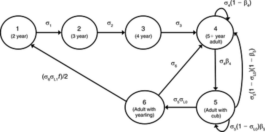
We follow the assumptions of Hunter et al. (2007, 2010) regarding the stage structure of polar bear life history (Figure 2), and the categorization of projection matrices as representing “good” or “bad” habitats depending on the sign of their λ (ie. positive/negative growth is good/bad). For every time t in our model, a projection matrix was chosen at random from one of the three “good” (2001 to 2003) or two “bad” (2004, 2005) habitat states, respectively. To explore a range of possible future climate scenarios, in our projections we vary the probability of a “bad” year (P(bad year) = q) from 0 to 1 in increments of 0.05. For all values of q, the probability of each of the “good” years is thus (1 − q)/3 and of bad years q/2. We ran 500 such simulations of 500 years (M = 500 and T = 500) for each value of q.
Figure 2.
Polar bear life cycle diagram (from Hunter et al. 2010)
At stationarity, the majority of individuals in the simulated population, for any sequence of environments, were in stage 4 (cubless adult females) (see Supplementary Figure E). Individuals in this stage also have the highest reproductive value, hence the dynamics of the population are dominated by parameters involving stage 4. In light of this dominance, and the extensive analysis of other vital rates already undertaken by Hunter et al (2007, 2010) we present mainly results regarding σ4, the survival rate of cubless adult females.
We focus primarily on the sensitivities for the variance in long term growth, then go on to discuss sensitivities for cumulative probability of quasi-extinction. We begin with the sensitivity of a and υ in the form of habitat-specific sensitivities, with a view to answering a question about management: is it wiser to concentrate on making the bad years better, or the good years excellent?
Results
Habitat Specific Sensitivities
We calculated the distinct effects on the mean and variance in stochastic growth of perturbing individual vital rates in each one of the five environmental states, separately. Think of the perturbation as a small increase, analogous to a successful conservation intervention. Thus, perturbations in habitats 4 and 5 amount to making a bad year less bad, while perturbations in habitats 1–3 essentially make good years even better (with respect to the perturbed rate).
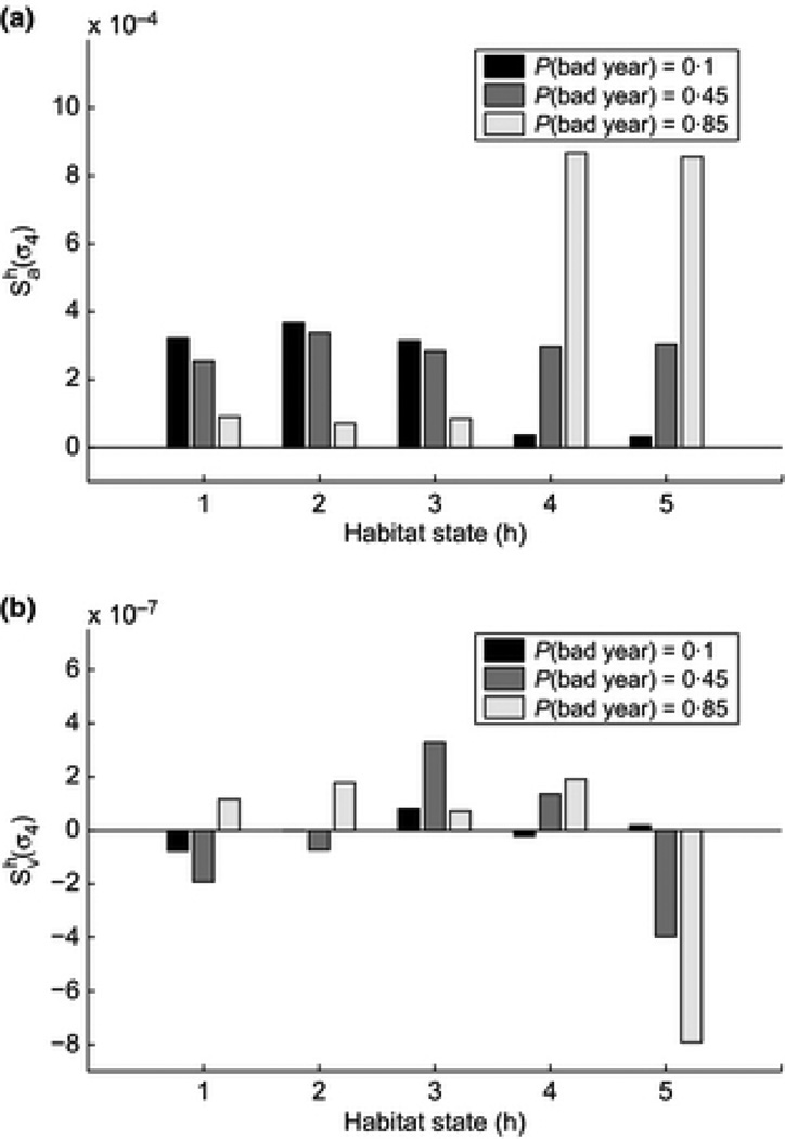
Given that our perturbations are of the bigger-is-better variety (increases to survival, fertility, breeding probability) we are unsurprised to find habitat-specific sensitivities of a are positive with respect to all vital rates (Figure 3).
Figure 3.
Habitat-specific sensitivity of a and υ to changes in cubless adult survival
The pattern of sensitivities of υ is much less straightforward to interpret (Figure 3). The standard expectation would be that regardless of environment, increasing survival should increase the stochastic growth rate and decrease its variance. Taking into account the division into “good” and “bad” years, one can partition the effect on υ into changes affecting variation within groups (good/bad) of habitats and between groups. Based on this divide, we then expect sensitivities of υ to be positive with respect to perturbation in good environments (making good years better increases the difference between “good” and “bad”) and negative in bad environments (since making bad years better decreases the difference between “good” and “bad” habitats). For the most part, this expectation is correct (Figure 3).
Deviations from this rule occur because the effect on υ of habitat specific perturbation also depends on the distribution of environments. If the sequence of environments is mostly good(bad) υ will be driven by variation in growth rates within good(bad) habitat groups. For example, we see that when good years are common (q = 0.15), is positive for perturbations in habitat 1 and 3, but negative in habitat 2. The observed values of σ4 in environments 1–3 were 0.9918, 0.9911 and 0.9662. Increasing survival in habitats 1 increases the variance between good years and overall variance as well, resulting in a positive sensitivity. Increasing survival in habitat 2 decreases the within-good-year variance, causing the negative sensitivity value. Increasing survival in habitat 3 decreases within-good-habitats variance, but increases the between-all-habitats variance, leading to an overall positive sensitivity value. From a conservation perspective then, this begs the question: is a management intervention that increases both the mean and the variance of population growth rate a desirable one?
Elasticities of the Mean and Variance of Stochastic Growth
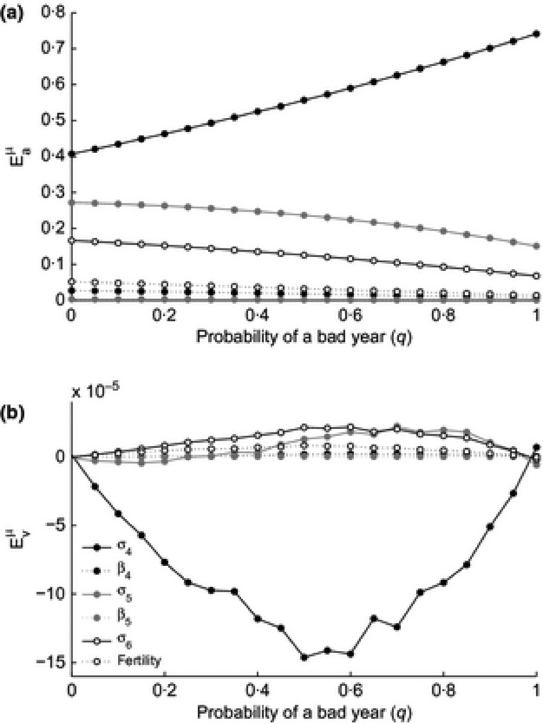
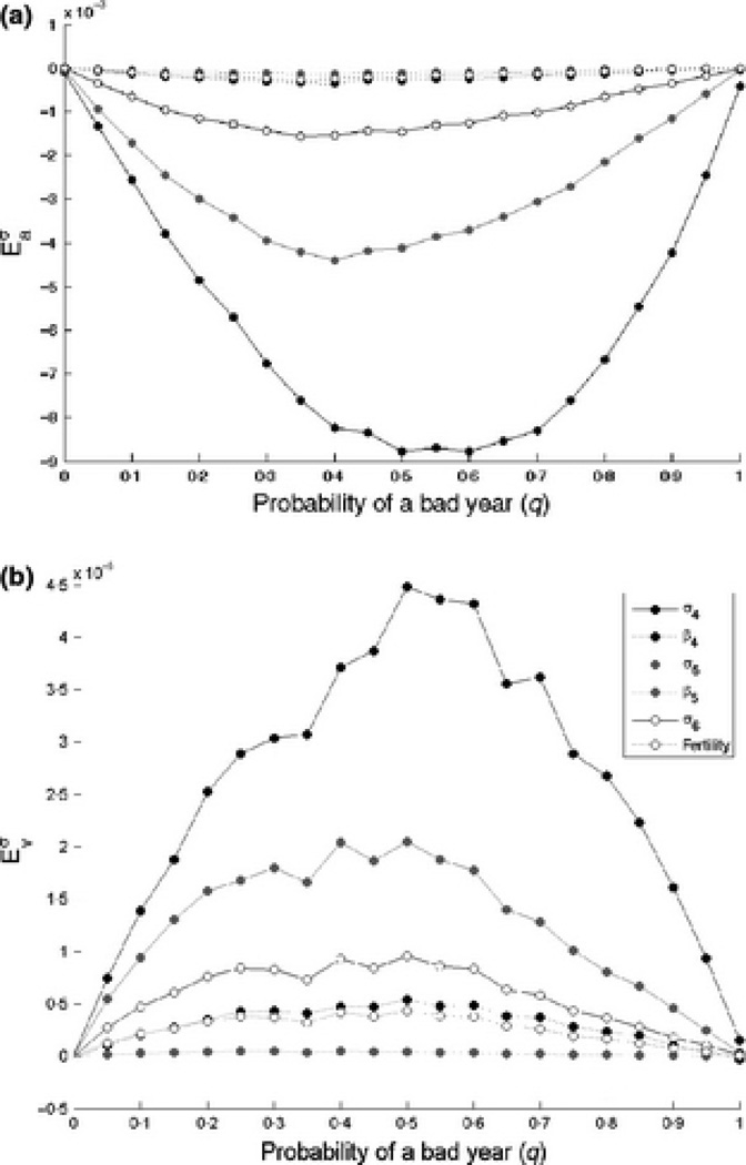
The naïve expectation here is that by perturbing the vital rates by the same amount in all habitats, the variance in growth rate would be unchanged since the variance between habitats is unchanged. However, changing a single vital rate alters the correlation structure of the matrices and the stable stage structure, resulting in some counterintuitive effects on υ. We found that with one notable exception, all perturbations increased υ, with the largest elasticities in the case of frequent (but not exclusively) bad years (Figure 4).
Figure 4.
Elasticity of a and υ to perturbation of the means of parameters
Perturbations that affect υ, must necessarily affect population growth rate to different degrees in the different habitats. Increasing σ4 in all habitats has a positive effect on the variance, but a larger effect in bad habitats than in good habitats, due to the larger occupancy of stage 4 in bad years. This disproportionate increase in growth in bad habitats leads to decreased variance between habitat states and thus a decrease in υ overall.
Unsurprisingly, increasing the variance of vital rates also increases υ (see Figure 5). The elasticity is again highest for σ4, and high frequency of bad environments. The elasticity to other parameters decreases as the frequency of bad environments goes up, again probably due to the skewing of stage structure towards all stage 4 individuals.
Figure 5.
Elasticity of a and υ to perturbation of the variance of parameters
Elasticities of Extinction
As noted by Hunter et al (2010), for all q > 0.15, the probability of quasi-extinction for this population is 1. In our simulations, a transition occurs (see Supplementary Figure F) as q increases, from very rare extinction (Pq ≃ 0) to certain extinction (Pq = 1). The transition to extinction is very abrupt and occurs very near to q = 0.165, (ie, where a ≃ 0: see Supplementary Figure G). Since the sensitivity of Pq depends on its value (Appendix C), SPq is always zero for this population. When q < 0.165, Pq = 0 and thus Spq = 0. When q > 0.165, extinction is certain and insensitive. We suspect this example system is unusual in its insensitivity of Pq to perturbation. The analysis of sensitivities for Pq has potential to be very informative for other systems with a broader parameter region of transition between growth and extinction risk.
In populations (such as these polar bears) where quasiextinction is certain, the best hope of conservation management is to find interventions that will extend the time to extinction. An intuitive way to find such interventions is to look at the sensitivities and elasticities of the cumulative probability of quasiextinction (SPq(t) and EPq(t)) to changes in vital rates. For example, if changing a vital rate results in strongly negative SPq(t), that means the change slows down the extinction process, causing extinction at time t to be less likely.
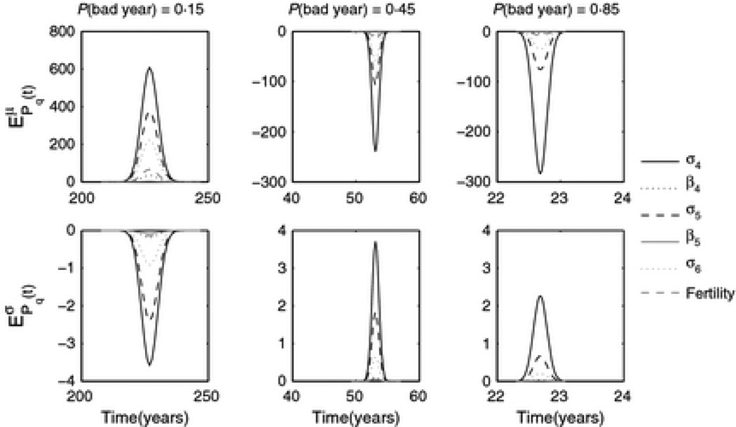
We find that, for all values of q, Pq(t) is most sensitive to changes in adult survival (σ4) and is only non-zero for t close to 〈Tq〉 (see Figure 6). When a > 0, increasing means of vital rates (top left panel) causes extinction to happen faster, and increased variance in vital rates (bottom left panel) causes extinction to slow down, both counterintuitive results at first glance. This results makes sense, however, if we consider that when a > 0 quasiextinction is unlikely but very rapid when it does occur. The only road to extinction is to experience a string of bad years at the very beginning of the process before growth takes over. For most of our simulations, a < 0, and EPq(t) is negative for increase to means and positive for increase to variance of vital rates. This implies that increasing mean adult survival slows down extinction, and increasing the variance of survival would speed it up. While the magnitude of EPq(t) is only weakly affected by q, the range of values of t over which EPq(t) is non-zero contracts sharply around 〈Tq〉 (which also decreases), as environmental quality degrades (higher q).
Figure 6.
Elasticity of Pq(t), probability of quasiextinction before time t, to changes in the means (top panel) and variances (bottom panel) of vital rates. Note that elasticity is maximal at 〈T〉, which has value (from left to right) 226.8, 53.1 and 22.6 years respectively. From left to right, values of a are 0.0203, −0.0868, −0.203
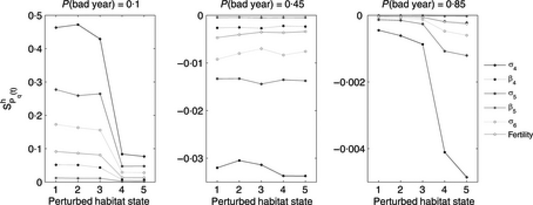
We also calculated habitat-specific sensitivities of Pq(t) for all vital rates, and here present results for a range of q. (Figure 7). When a > 0 (leftmost panel), sensitivities are larger for interventions in good years than in bad, and this pattern slowly reverses as a becomes negative. When a is negative (center and right panels) sensitivities are most strongly negative for perturbations in bad years. This result implies that in management terms it is most advantageous to protect bears in bad years, which agrees what we observed in the habitat specific sensitivities of a and υ (Figure 3). Unlike and , the magnitude of decreases rapidly as q increases.
Figure 7.
Sensitivity of Pq(t), probability of quasiextinction before time t, to habitat-specific changes in vital rates. From left to right, values of a are 0.0203, −0.0868, −0.203. Sensitivities shown are all for the case t = 〈T〉, to the nearest year, (from left to right) 227, 53 and 23 years respectively.
Taken together our results suggest that for this population of bears, Pq(t) could be ameliorated by management intervention even in the worst-case range of future environments (q ≃ 1), although sensitivites are of course highest when a is only weakly negative. It is most important to note that SPq(t) is a function of a, υ, Sa and Sυ, so managing to maximize time to extinction must factor in population growth and its variance, as well as the sensitivities for both.
Discussion
Conclusions: Beyond the mean
We have given an exact method for calculating the stochastic sensitivity of the variance in long term population growth, and demonstrated its potential utility in application to questions in conservation biology. This variance sensitivity yields new information about the variance, and also makes possible the calculation of sensitivities for the probability of quasi-extinction.
Increase in the variance of a necessarily increases the width of confidence bounds around estimates of population size, population growth, probability of and time to quasiextinction (Doak et al., 1994; Lewontin and Cohen, D, 1969) especially over short time intervals. Thus, sensitivity of the variance in growth is a valuable and necessary addition to the analysis toolkit for populations at risk. Our analysis has demonstrated that mean and variance sensitivities and elasticities do not always behave in an intuitively obvious manner. Perturbations that increase a can also increase υ (Figures 3–5), so particularly in highly variable environments it is important to go beyond simple sensitivity analyses of a.
Our results for habitat-specific sensitivities of population growth imply that it is useful to decompose the overall variance into contributions within and between groups of similar habitats. For example, we found that increasing survival in habitat 3 decreases within-good-habitats variance, but increases the between-all-habitats variance, resulting in positive sensitivity value (Figure 3). From a conservation perspective then, this begs the question: is a management intervention that increases both the mean and the variance of population growth rate a desirable one? That depends entirely on the magnitude of both increases, and on the environmental variation driving the given system.
Our new sensitivity for the variance in population growth allows another new calculation that helps tease apart the effects of a and υ on population processes: sensitivity of the cumulative extinction probability Pq(t). This new calculation provides a quantitative way to assess how a given management intervention will affect the extinction process. Previously such sensitivity analyses would have had to be done by extensive numerical simulation, or be omitted in favour of qualitative insights from sensitivity analysis of a alone. Considering that the extinction process depends in complicated ways on both the mean and variance of population growth, our calculation for SPq(t) provides a valuable new quantitative tool to produce more nuanced analyses of population dynamics.
Considering the magnitude of projected climate variability in the next century, previous work finds that quasiextinction is certain for our example population (Hunter et al., 2007). Given this vulnerability of polar bears to climatic variability, even though the magnitudes of our variance sensitivities are small, management efforts might still benefit from taking into consideration the effects of proposed interventions on υ as well as on a. In particular, we note that even small changes to υ can have considerable effects on cumulative probability of quasiextinction and its sensitivities. In general, given the potentially counterintuitive (and counterproductive) behaviour of both growth and extinction sensitivities, and the trend towards increasing environmental uncertainty, we suspect many management programs could be improved by a a whole-distribution approach to sensitivity analysis.
These new sensitivities should also be useful in many other population dynamics applications. We are particulary interested in exploring the applications of variance sensitivities to evolutionary questions. Intuition suggests that natural selection should favour any change that increase a or decreases υ. But, what if there are cases where a and υ respond differently to the same change in a particular vital rate? How do we interpret a change in vital rates that increases both the mean and the variance of growth? In an increasingly variable world, it is unwise to treat the mean of a stochastic process alone as giving a full description of dynamics. The inclusion of variance sensitivites in future studies will move us towards a more complete understanding of population dynamics problems.
Supplementary Material
Acknowledgements
We thank Duncan Gillespie, Tim Coulson and Carol Horvitz for helpful discussion, and David Koons and an anonymous reviewer for helpful comments on the manuscript. This project is funded by the National Institutes of Health grants AG22500 and AG039345 to S.T.
References
- Aberg P, Svensson CJ, Caswell H, Pavia H. Environment-specific elasticity and sensitivity analysis of the stochastic growth rate. Ecological Modelling. 2009;220:605–610. [Google Scholar]
- Beissinger SR, McCullough DR. Population viability analysis. University of Chicago Press; 2002. [Google Scholar]
- Boyce MS, Haridas CV, Lee CT. Demography in an increasingly variable world. Trends Ecol. Evol. 2006;21:141–148. doi: 10.1016/j.tree.2005.11.018. [DOI] [PubMed] [Google Scholar]
- Caswell H. Matrix population models, vol. 2nd. Sunderland, USA: Sinauer Associates; 2001. [Google Scholar]
- Caswell H. Sensitivity analysis of the stochastic growth rate: Three extensions. Australian & New Zealand Journal of Statistics. 2005;47:75–85. [Google Scholar]
- Cohen JE. Ergodic theorems in demography. Bulletin (New Series) of the American Mathematical Society. 1979;1:275–295. [Google Scholar]
- Dennis B, Munholland PL, Scott JM. Estimation of growth and extinction parameters for endangered species. Ecological Monographs. 1991;61:115–143. [Google Scholar]
- Doak DF, Kareiva P, Kleptetka B. Modeling population viability for the desert tortoise in the western mojave desert. Ecological Applications. 1994;4:446–460. [Google Scholar]
- Durner GM, Amstrup SC, Neilson R, McDonald T. The use of sea ice habitat by female polar bears in the beaufort sea. OSC Report. 2004 [Google Scholar]
- Ellner SP, Rees M. Integral projection models for species with complex demography. The American Naturalist. 2006;167:410–428. doi: 10.1086/499438. [DOI] [PubMed] [Google Scholar]
- Engen S, Lande R, Saether BE, Bregnballe T. Estimating the pattern of synchrony in fluctuating populations. Journal of Animal Ecology. 2005;74:601–611. [Google Scholar]
- Engen S, Lande R, Saether BE, Gienapp P. Estimating the ratio of effective to actual size of an age-structured population from individual demographic data. Journal of Evolutionary Biology. 2010;23:1148–1158. doi: 10.1111/j.1420-9101.2010.01979.x. [DOI] [PubMed] [Google Scholar]
- Ezard THG, Gaillard J, Crawley MJ, Coulson T. Habitat dependence and correlations between elasticities of LongTerm growth rates. The American Naturalist. 2008;172:424–430. doi: 10.1086/589897. [DOI] [PubMed] [Google Scholar]
- Hunter CM, Caswell H, Runge MC, Regehr EV, Amstrup SC, Stirling I. Polar bears in the southern beaufort sea II: demography and population growth in relation to sea ice conditions. Administrative report, US Geological Survey. 2007 [Google Scholar]
- Hunter CM, Caswell H, Runge MC, Regehr EV, Amstrup SC, Stirling I. Climate change threatens polar bear populations: a stochastic demographic analysis. Ecology. 2010;91:2883–2897. doi: 10.1890/09-1641.1. [DOI] [PubMed] [Google Scholar]
- Lande R, Engen S, Saether B-E, Coulson T. Estimating density dependence from time series of population age structure. The American Naturalist. 2006;168:76–87. doi: 10.1086/504851. [DOI] [PubMed] [Google Scholar]
- Lande R, Engen S, Sther B-E. Stochastic population dynamics in ecology and conservation. Oxford University Press; 2003. [Google Scholar]
- Lande R, Orzack SH. Extinction dynamics of age-structured populations in a fluctuating environment. Proceedings of the National Academy of Sciences. 1988;85:7418–7421. doi: 10.1073/pnas.85.19.7418. [DOI] [PMC free article] [PubMed] [Google Scholar]
- Lange K, Holmes W. Stochastic stable population growth. Journal of Applied Probability. 1981;18:325–334. [PubMed] [Google Scholar]
- Lebreton J. Demographic models for subdivided populations: The renewal equation approach. Theoretical Population Biology. 1996;49:291–313. doi: 10.1006/tpbi.1996.0015. [DOI] [PubMed] [Google Scholar]
- Lee RD, Tuljapurkar SD. Stochastic population forecasts for the united states: Beyond high, medium, and low. Journal of the American Statistical Association. 1994;89:1175–1189. [PubMed] [Google Scholar]
- Lewontin RC, Cohen D. On population growth in a randomly varying environment. Proceedings of the National Academy of Sciences of the United States of America. 1969;62:1056–1066. doi: 10.1073/pnas.62.4.1056. [DOI] [PMC free article] [PubMed] [Google Scholar]
- Morris WF, Doak DF. Quantitative conservation biology: theory and practice of population viability analysis. Sinauer Associates; 2002. [Google Scholar]
- Morris WF, Pfister CA, Tuljapurkar S, Haridas CV, Boggs CL, Boyce MS, Bruna EM, Church DR, Coulson T, Doak DF, Forsyth S, Gaillard JM, Horvitz CC, Kalisz S, Kendall BE, Knight TM, Lee CT, Menges ES. Longevity can buffer plant and animal populations against changing climatic variability. Ecology. 2008;89:19–25. doi: 10.1890/07-0774.1. [DOI] [PubMed] [Google Scholar]
- Saether BE, Lillegard M, Grotan V, Filli F, Engen S. Predicting fluctuations of reintroduced ibex populations: the importance of density dependence, environmental stochasticity and uncertain population estimates. Journal of Animal Ecology. 2007;76:326–336. doi: 10.1111/j.1365-2656.2006.01197.x. [DOI] [PubMed] [Google Scholar]
- Steinsaltz D, Tuljapurkar S, Horvitz C. Derivatives of the stochastic growth rate. Theoretical Population Biology. 2011;80:1–15. doi: 10.1016/j.tpb.2011.03.004. [DOI] [PMC free article] [PubMed] [Google Scholar]
- Stirling I, Lunn NJ, Iacozza J, Elliott C, Obbard M. Polar bear distribution and abundance on the southwestern hudson bay coast during open water season, in relation to population trends and annual ice patterns. Arctic. 2004;57:15–26. [Google Scholar]
- Tuljapurkar S. Population Dynamics in Variable Environments. Springer-Verlag; 1990. [Google Scholar]
- Tuljapurkar S, Gaillard J-M, Coulson T. From stochastic environments to life histories and back. Philosophical Transactions of the Royal Society B: Biological Sciences. 2009;364:1499–1509. doi: 10.1098/rstb.2009.0021. [DOI] [PMC free article] [PubMed] [Google Scholar]
- Tuljapurkar S, Horvitz CC. From stage to age in variable environments: Life expectancy and survivorship. Ecology. 2006;87:1497–1509. doi: 10.1890/0012-9658(2006)87[1497:fstaiv]2.0.co;2. [DOI] [PubMed] [Google Scholar]
- Tuljapurkar S, Horvitz CC, Pascarella JB. The many growth rates and elasticities of populations in random environments. Am. Nat. 2003;162:489–502. doi: 10.1086/378648. [DOI] [PubMed] [Google Scholar]
- Tuljapurkar S, Orzack SH. Population dynamics in variable environments i. long-run growth rates and extinction. Theoretical Population Biology. 1980;18:314–342. [Google Scholar]
- Tuljapurkar SD. Population dynamics in variable environments. III. evolutionary dynamics of r-selection. Theoretical Population Biology. 1982;21:141–165. [Google Scholar]
Associated Data
This section collects any data citations, data availability statements, or supplementary materials included in this article.


