Efficient estimation of Weber’s W

Abstract

Many studies rely on estimation of Weber ratios (W) in order to quantify the acuity an individual’s approximate number system. This paper discusses several problems encountered in estimating W using the standard methods, most notably the low power and inefficiency of standard methods. Through simulation, this work shows that W can best be estimated in a Bayesian framework that uses an inverse (1/W) prior. This beneficially balances a bias/variance trade-off and, when used with MAP estimation is extremely simple to implement, requiring only a single term added to the function used to fit W. Use of this scheme substantially improves statistical power in examining correlates of W.

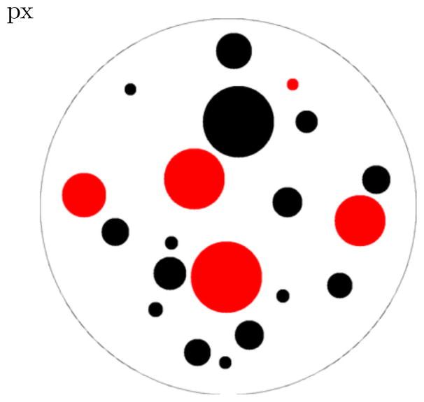
A common task in the study of numerical cognition is estimating the acuity of the approximate number system (Dehaene, 1997). This system is active in representing and comparing numerical magnitudes that are too large to exactly count. A typical kind of stimulus is shown in Figure 1, where participants might be asked to determine if there are more red or black dots, but the total area, min, and max sizes of these colored dots are equal, leading participants to use number rather than these other correlated dimensions to complete the comparison.¹ In this domain, human performance follows Weber’s law, a more general psychophysical finding that the just noticeable difference between stimuli scales with their magnitude. Higher intensity stimuli—here, higher numbers—appear to be represented with lower absolute fidelity, but constant fidelity relative to their magnitude. Since Fechner (1860), some have characterized the psychological scaling of numbers as logarithmic, with the effective psychological distance between representations of numbers n and m scaling as n/m (Dehaene, 1997 ; Masin, Zudini, & Antonelli, 2009 ; Nieder, Freedman, & Miller, 2002 ; Nieder & Miller, 2004 ; Nieder & Merten, 2007 ; Nieder & Dehaene, 2009 ; Portugal & Svaiter, 2011 ; Sun, Wang, Goyal, & Varshney, 2012). Alternatively, others have characterized numerical representations with a close but distinct alternative: a linear scale with linearly increasing error (standard deviation) on the representations, known as scale variability (Gibbon, 1977 ; Meck & Church, 1983 ; Whalen, Gallistel, & Gelman, 1999 ; Gallistel & Gelman, 1992). This latter formalization motivates characterizing an individual’s behavior by fitting a single parameter W that determines how the standard deviation of a representation scales with its magnitude: each numerosity n is represented with a standard deviation of W · n. In, tasks where subjects must compare two magnitudes, n₁ and n₂, this psychophysics can be formalized (e.g. Halberda, Mazzocco, & Feigenson, 2008) by fitting W to their observed accuracy via,

Figure 1.

An example stimulus for an approximate number task, where participants must rapidly decide if there are more black or red dots. The areas, min sizes, and max sizes between the dots are controlled, and the dots are intermixed in order to discourage strategies based on area.

$$P(\mathit{correct}\mid W,n_1,n_2)=\mathrm{\Phi }\left[\frac{\mid n_1-n_2\mid }{W·\sqrt{n_1^2+n_2^2}}\right].$$ (1)

In this equation, Φ is the cumulative normal distribution function. The value in (1) gives the probability that a sample from a normal distribution centered at n₁ with standard deviation W · n₁ will be larger than a sample from a distribution centered at n₂ with standard deviation W · n₂ (for n₁ > n₂). The values n₁ and n₂ are fixed by the experimental design; the observed probability of answering accurately is measured behaviorally; and W is treated as a free variable that characterizes the acuity of the psychophysical system. As W → 0, the standard deviation of each representation goes to 0, and so accuracy will increase. As W gets large, the denominator in (1) goes to zero and accuracy approaches the chance rate of 50%.

The precise value of W for an individual is often treated as a core measurement of the approximate system’s acuity (though see Gilmore, Attridge, & Inglis, 2011), and is compellingly related to other domains: for instance, it correlates with exact symbolic math performance (Halberda et al., 2008 ; Mussolin, Nys, & Leybaert, 2012 ; Bonny & Lourenco, 2013), its value changes over development and age (Halberda & Feigenson, 2008 ; Halberda, Ly, Wilmer, Naiman, & Germine, 2012), and is shared among human groups (Pica, Lemer, Izard, & Dehaene, 2004 ; Dehaene, Izard, Spelke, & Pica, 2008 ; Frank, Fedorenko, & Gibson, 2008).

Despite the importance of W as a psychophysical quantity, little work has examined the most efficient practices for estimating it from behavioral data. The present paper evaluates several different techniques for estimating W in order to determine which are most efficient. Since the problem of determining W is at its core a statistical inference problem—one of determining a psychophysical variable that is not directly observable—our approach is framed in terms of Bayesian inference. This work draws on Bayesian tools and ways of thinking that have increasingly become popular in psychology (Kruschke, 2010b, 2010a, 2010c). In the context of the approximate number system, the first work to infer Weber ratios through Bayesian data analysis was (Lee & Sarnecka, 2010, 2011), who used Bayesian techniques to show that children’s performance in number tasks is better described by discrete and exact knower-level theories (e.g. Carey, 2009) than ones based in the approximate number system.

With a Bayesian framing, we are interested in P(W | D), the probability that any value for W is the true one, given some observed behavioral data D. By Bayes rule, this can be found via P(W | D) ∝ P(D | W) · P(W), where P(D | W) is the likelihood of the data given a particular W and P(W) is a prior expectation about what W are likely. In fact, P(D | W) is already well-established in the literature: the likelihood W assigns to the data is given by (1), which quantifies the probability that a subject would answer correctly on each given trial for any choice of W.² The key additional part to the Bayesian setting is therefore the prior P(W), which is classically a quantification of our expectations about W before any data is observed.

The choice of P(W) presents a clear challenge. There are many qualitatively different priors that one might choose and, in this case, no clear theoretical reasons for preferring one over another. These types of priors include those that are invariant to re-parameterization (e.g. Jeffreys’ priors), priors that allow the data to have the strongest influence on the posterior (reference priors), and those that could capture any knowledge we have about likely values of W (informative priors). Or, we might choose P(W) ∝ 1, corresponding to “flat” expectations about the value of W, in which case the prior does not affect our inferences. This naturally raises the question of which prior is best ; can correctly calibrating our expectations about W lead to better inferences, and thus better quality in studies that depend on W?

To be clear, the question of which prior is “best” is a little unusual from the viewpoint of Bayesian inference, since the prior is usually assumed from the get-go. However, there are criteria through which priors can be judged. Some recent work in psychology has argued through simulation that priors should not be tuned to real-world frequencies, since inferences with more entropic priors tend to yield more accurate posterior distributions (Feldman, 2013). In applied work on Bayesian estimators, the performance of different priors is often compared through simulations that quantify, for instance, the error between a simulated value and its estimated posterior value under each prior (e.g. Tibshirani, 1996 ; Park & Casella, 2008 ; Hans, 2011 ; Bhattacharya, Pati, Pillai, & Dunson, 2012 ; Armagan, Dunson, & Lee, 2013 ; Pati, Bhattacharya, Pillai, Dunson, et al., 2014).³ Here, we follow the same basic approach by simulating behavioral data and comparing priors to see which creates an inferential setup that best recovers the true generating value of W, under various assumptions about the best properties for an estimate to have. The primary result is that W can be better estimated than (1) by incorporating a prior—in particular, a 1/W prior—and using a simple MAP (maximum a posteriori) estimate of the posterior mode. As such, this domain provides one place for Bayesian ideas to find simple, immediate, nearly-effortless, quantifiable improvements in scientific practice.

The basic problem with W

The essential challenge in estimating W in the psychophysics of number is that W plays roughly the same role as a standard deviation. As such, the range of possible W is bounded (W ≥ 0) and typical human adults are near the “low” end of this scale, considerably less than 1. A result of this is that the reliability of an estimate of W will depend on its value, a situation that violates the assumptions of essentially all standard statistical analyses (e.g. t-tests, ANOVA, regression, correlation, factor analysis, etc.)

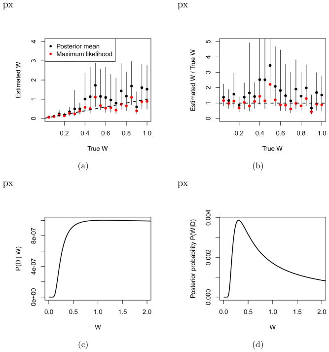
Figure 2(a) illustrates the problem. The x-axis here shows a true value of W, which was used to generate simulate data consisting of 50 responses in a 2-up-1-down staircased design with n₂ always set to n₁ + 1. This simulation is used for all results in the paper, however the results presented are robust to other designs and situations, including exhaustive testing of numerosities (see Appendix ) and situations where additional noise factors decrease accuracy at random (see Appendix ). In Figure 2(a), a posterior mean estimated W is shown by black dots using a uniform prior⁴, and the 95% highest posterior density region (specifying the region where the estimation puts 95% of its confidence mass) is shown by the black error bars. This range show the set of values we should consider to be reasonably likely for each subject, over and above the posterior point estimate in black. For comparison, a ML fit—using just (1)—is shown in red.

Figure 2.

(a) Values of W estimated from single simulated subjects at various true values of W, running 50 steps of a 2-up-1-down staircase design. Points show posterior mean (black) and maximum likelihood (red) fits to the data. Error bars show 95% highest posterior density intervals. The dotted lines represent y = x, corresponding to perfect estimation of W. (b) Same data on a proportional scale to show the relative error of estimate at each W. (c) The likelihood given by (1) on a simple data set, showing that high values of W all make the data approximately equally likely. There is little hope of accurately estimating high W. (d) This can be corrected by introduction of a weak prior exhibiting a clear maximum (here, a MAP value). Whether this maximum is inferentially useful is the topic of the next section.

This figure illustrates several key features of estimating W. First, the error in the estimate depends on the value of W: higher Ws not only have greater likely ranges, but also greater scatter of the mean (circle) about the line y = x. This increasing variance is seen in both the mean (black) and ML fits, and Figure 2(b) suggests even the relative error may increase as W grows.

Because Bayesian inference represents optimal probabilistic inference relative to its assumptions, we may take the error bars here as normative, reflecting the certainty we should have about the value of W given the data. For instance, in this figure the error bars almost all overlap with the line y = x, which would be correct estimation of W. From this viewpoint, the increasing error bars show that we should have more uncertainty about W when it is large than when it is small. The data is simply less informative about high values of W when it is in this range. This is true in spite of the fact that the same number of data points are gathered for each simulated subject.

The reason for this increasing error of estimation is very simple: equation (1) becomes very “flat” for high W due to the fact that 1/W approacher zero for high values. This is shown in Figure 2(c), giving the value of (1) for various W on a simple data set consisting of a ten correct answers on (n₁, n₂) = (6, 7) and ten incorrect answers on (7, 8). When W is high, it predicts correct answers at the chance 50% rate and it matters very little which high value of W is chosen (e.g. W = 1.0 vs W = 2.0), as the line largely flattens out for high W. As such, choosing W to optimize (1) is in the best case error-prone, and the worst case meaningless for these high values. Figure 2(d) shows what happens when a prior P(W) ∝ 1/W is introduced. Now, we see a clear maximum because although the likelihood is flat, the prior is decreasing, so the posterior (shown) has a clear mode. The “optimal” (maximum) value of the line in Figure 2(d) might provide a good estimate of the true W.

The next two sections address two concerns that Figure 2(a) should raise. First, one might wonder what type of inferential setup would best allow us to estimate W. In this figure, the maximum likelihood estimation certainly looks better than posterior mean estimation. Section considers other types of estimation, different priors on W, and different measures of the effectiveness of an estimate. Section examines the impact that improved estimation has on finding correlates W, as well as the consequences of the fact that our ability to estimate W changes with the magnitude of W itself.

Efficient estimation of W

In general, use of the full Bayesian posterior on W provides a full characterization of our beliefs, and should be used for optimal inferences about the relationship between W and other variables. However, most common statistical tools do not handle posterior distributions on variables but rather only handle single measurements (e.g. a point estimate of W). Here, we will assume that we summarize the posterior in W with a single point estimate since this is likely the way the variable will be used in the literature. For each choice of prior, we consider several different quantitative measures of how “good” an estimate a point estimate is, using several different point-estimate summaries of the posterior (e.g. the mean, median, and mode). The analysis compares each to the standard ML fitting used by (1).

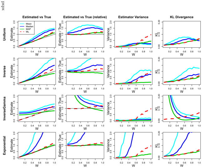
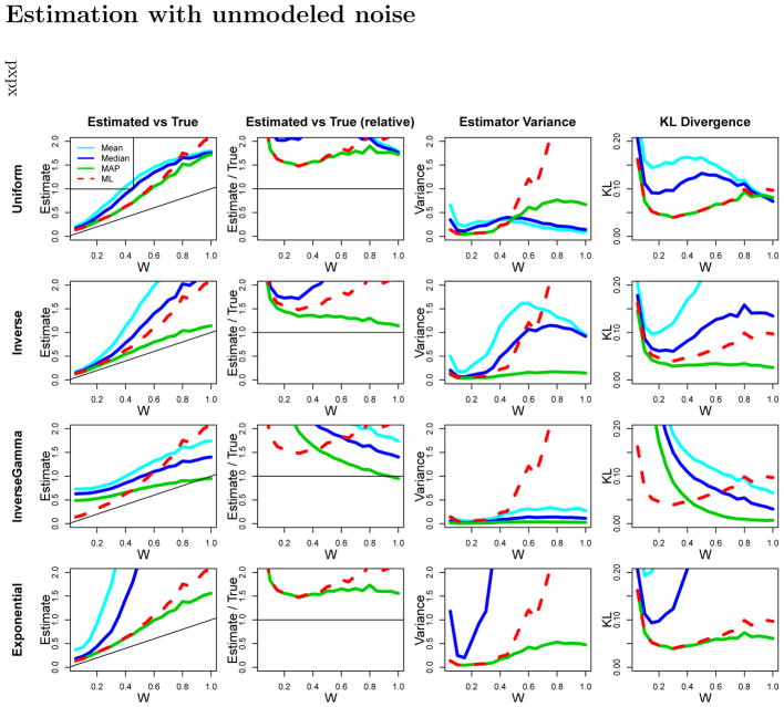
Figure 3 shows estimation of W for several priors and point estimate summaries of the posterior, across four different measures of an estimate’s quality. Each subplot shows the true W on the x-axis. The first column shows on the mean estimated Ŵ for each W, across 1000 simulated subjects, using the 2-up-1-down setup used in Figure 2(a). Recovery of the true W here would correspond to all points lying on the line y = x. The second column shows the relative estimation, Ŵ/W at each value of W, providing a measure of relative bias. The third column shows the variance in the estimate of Ŵ, V ar[ Ŵ | W]. Lower values correspond to more efficient estimators of W, meaning that they more often have Ŵ close to W. The fourth column shows the difference between the estimate and the true value according to an information-theoretic loss function. Assuming that a person’s representation of a number n is Normal(n, Wn), we may capture the effective quality of an estimate Ŵ for the underlying psychological theory by looking at the “distance” between the true distribution Normal(n, Wn) and the estimated distribution Normal(n, Ŵ n). One natural quantification of the distance between distributions is the KL-divergence (see Cover & Thomas, 2006). The fourth column shows the KL-divergence⁵ (higher is worse), quantifying in an information-theoretic sense, how much an estimated Ŵ matters in terms of the psychological model thought to underlie Weber ratios.

Figure 3.

Estimation properties of W for various priors (rows). The first column shows the mean estimate Ŵ as a function of the true value W. Unbiased estimation follows the line y = x shown in black. The second column shows the relative error of this estimate Ŵ/W. Unbiased estimation follows the line y = 1, shown in black. The third column shows the variance of the estimated Ŵ as a function of the true W. The fourth column shows a loss function based on the KL-divergence in the underlying psychophysical model.

The rows in this figure correspond to four different sets of priors P(W). The first row is a uniform prior P(W) ∝ 1 on the interval W ∈ [0, 3]. Because this prior doesn’t affect the value of the posterior in this range, it has that P(W | D) = P(D | W) meaning that estimation is essentially the same as in ML fitting of (1). However, unlike (1), the Bayesian setup still allows computation of the variability in the estimated W, as well as posterior means (light blue), and medians (dark blue), in addition to MAPs (green). For comparison, each plot also shows the maximum likelihood fit (1) in red⁶.

The second row shows an inverse prior P(W) ∝ 1/W. This prior would be the Jeffreys’ prior for estimation of a normal standard deviation⁷, to which W is closely related, although the inverse prior is not a Jeffreys’ prior for the current likelihood, which appears to be fairly complex. The inverse prior strongly prefers low W.

The third row shows another standard prior, an inverse-Gamma prior. This prior is often a convenient one for use in Bayesian estimation of standard deviations because it is conjugate to the normal, meaning that the posterior is of the same form as the prior, allowing efficient inference strategies and analytical computation. The shown inverse-Gamma uses a shape parameter α = 1 and scale β = 1, yielding a peak in the prior at 0.5. The shape of the inverse-Gamma used here corresponds to some strong expectations that W is neither too small nor too large, but approximately in the right range. Because of this, this prior pulls smaller W higher, and higher W lower, as shown by the second column plot with estimates above the line for low W and below the line for high W.

The fourth row shows an exponential prior P(W) = λe^−λW for λ = 0.1, a value chosen by informal experimentation. This corresponds to substantial expectations that W is small, with pull downwards instead of upwards for small W.

From Figure 3 we are able to read off the most efficient scheme for estimating W under a range of possible considerations. For instance, we may seek a prior that gives rise to a posterior with the lowest mean or median KL-Divergence, meaning the row for which the light and dark blue lines respectively are lowest in the fourth column. Or, we may commit to a uniform prior (first row) and ask whether posterior Means, Medians, or MAPs provide the best summary of the posterior under each of these measures (likely, MAP). Much more globally, however, we can look across this figure and try to determine which estimation scheme—which prior (column) and posterior summary (line type)—together provide the best overall estimate. In general, we should seek a scheme that (i) falls along the line (y = x) in the first column (low bias), (ii) falls along the line y = 1 in the second (low relative error), (iii) has the minimum value for a range of W in the third column (low variance), and (iv) has low values for KL-divergence (the errors in Ŵ “matter least” in terms of the psychological theory). With these criteria, the mean and median estimates of W are not very efficient for any prior: they are high variance, particularly compared to the ML and MAP fits, as well as substantially biased. Intuitively, this comes from the shape of the posterior distribution on W: the skew (Figure 2(d)) means that the mean of the posterior may be substantially different than the true value. The ML fits tend to have high relative variance for W > 0.5. In general, MAP estimation with the inverse 1/W prior (green line, second row) is a clear winner, with very little bias (the prior does not affect the posterior “too much”) and low variance across all these tested W. This also performs as well as ML fits in terms of KL-Divergence. A close overall second place is the weak exponential prior. Both demonstrate a beneficial bias-variance trade-off: by introducing a small amount of bias in the estimates we can substantially decrease the variance of the estimated W. Appendices and show that similar improvements in estimation are found in non-staircased designs and where there are additional sources of unmodeled noise.

The success of the MAP estimator over the mean may have more general consequences for Bayesian data analysis in situations like these where the likelihood is relatively flat (e.g Figure 2(c)). Here, the flatness of the likelihood leads to still a broad posterior (Figure 2(d)). This is what leads posterior mean estimates of W to be much less useful than posterior MAP estimates.

It is important to point out that the present analysis has assumed each subject’s W is estimated independently from any others. This assumption is a simplification that accords with standard ML fitting. Even better estimation could likely be developed using a hierarchical model in which the group distribution of W is estimated for a number of subjects, and those subject estimates are informed by the group distribution. This approach, for instance, leads to much more powerful and sensible results in the domain of mixed-effect regression (Gelman & Hill, 2007). It is beyond the scope of the current paper to develop such a model, but hierarchical approaches will likely prove beneficial in many domains, particularly where distinct group mean Ws must be compared.

Power and heteroskedasticity in estimating W

We next show that improved estimates of W lead to improved power in looking for correlates of W, a fact that may have consequences for studies that examine factors that do and—especially—do not correlate with approximate number acuity. A closely related issue to statistical power is the impact of the inherent variability in our estimation of W. In different situations, ignoring the property that higher W are estimated higher noise can lead to either reduced power (type-I errors) or anticonservativity (type-II errors) (see Hayes & Cai, 2007).

Figure 4(a) shows one simple simulation assessing correlates of W. In each simulated experiment, a predictor x has been sampled that has a coefficient of determination R² with the true value of W (not Ŵ). Then, 30 subjects were sampled at random from the Weber value range used in the previous simulation study (50 responses each, staircased n/(n +1) design). These figures show how commonly (y-axis) statistically significant effects of x on Ŵ were found at p < 0.05 as a function of R² (x-axis), over the course of 5000 simulated experiments. Statistically powerful tests (lower type-I error rate) will increase faster in Figure 4(a) as R² increases; statistically anti-conservative tests will have a value greater than 0.05 when R² = 0 (the null hypothesis).

Figure 4.

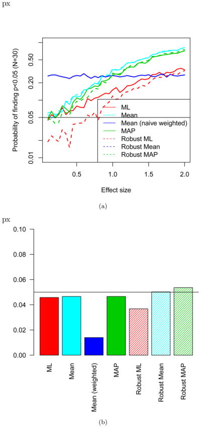
(a) A power analysis showing the probability of finding a correlation between a predictor with the given correlation (x-axis) to the true Weber ratio W. (b) The false positive (type II) error rate for various estimators and analyses when considering correlations.

Several different analysis techniques are shown. First, the red solid line shows the maximum likelihood estimator analyzed with a simple linear regression Ŵ ~ x. The light blue and green lines show the mean and MAP estimators for W respectively, also analyzed with a simple linear regression. The dark blue line corresponds to a weighted regression where the points have been weighted by their reliability.⁸ The dotted lines correspond to use of heteroskedasticity-consistent estimators, via the sandwich package in R (Zeileis, 2004). This technique, developed in the econometric literature, allows computation of standard errors and p-values in a way that is robust to violations of homoskedasticity.

This figure makes it clear first that the ML estimator typically used is underpowered relative to mean or MAP estimators. This is most apparent for R²s above 0.3 or so, for which the MAP estimators have a much higher probability of detecting an effect than the ML estimators. This has important consequences for null results, or comparisons between groups where one shows a significant difference in W and another does not, particularly when such comparison are (incorrectly) not analyzed as interactions (for discussion of this error, see Nieuwenhuis, Forstmann, & Wagenmakers, 2011). The increased power for non-ML estimations seen in Figure 4(a) indicates that such estimators should be strongly preferred by researchers and reviewers.

The value for R² = 0 (left end of the plot) corresponds to the null hypothesis of no relationship. For clarity, the value of the lines have been replotted in Figure 4(b). Bars above the line 0.05 would reflect statistical anticonservativity, where the method has a greater than 5% chance of finding an effect when the null (R² = 0) is true. This figure shows that these methods essentially do not increase the type-II error rates with a possible very minor anticonservativity for robust regressions with the MAP estimate.⁹ Use of the weighted regression is particularly conservative. In general, the heteroskedasticity found in estimating W is not likely to cause problems when un-modeled in this simple correlational analysis.

Conclusion

This paper has examined estimation of W in the context of a number of common considerations. Simulations here have shown that MAP estimation with a 1/W prior allows efficient estimation across a range of W (Figure 3) and considering a variety of important features of good estimation. This scheme introduces a small bias on W that helps to correct the large uncertainty about W that occurs for higher values. Its use leads to statistical tests that are more powerful than the standard maximum likelihood fits given by (1). When used in simple correlational analyses, many of the standard analysis techniques do not introduce increased type-II error rates, despite the heteroskedasticity inherent in estimating W.

Instructions for estimation

The recommended 1/W prior is extremely easy to use, including only a –logW term in addition to the log likelihood that is typically fit. If subjects were shown pairs of numbers (a_i, b_i) and r_i is a binary variable indicating whether they responded correctly (r_i = 1) or incorrectly (r_i = 0), we can fit W to maximize

$$-logW+\sum _{i}log\left(r_i·\mathrm{\Phi }\left[\frac{\mid a_i-b_i\mid }{W·\sqrt{a_i^2+b_i^2}}\right]+(1-r_i)·\left(1-\mathrm{\Phi }\left[\frac{\mid a_i-b_i\mid }{W·\sqrt{a_i^2+b_i^2}}\right]\right)\right).$$ (2)

In R (R Core Team, 2013), we can estimate W via

    optimize (function (W) {
        pcorrect <– pnorm(abs(ai–bi)/(W * sqrt (ai **2+bi**2)))
        –log (W) + sum(log (ifelse (ri, pcorrect, 1–pcorrect)))
    }, maximum=TRUE, interval=c (0, 3))

where ai, bi and ri are vectors of a_i, b_i, and r_i respectively. Note that the use of MAP estimation here (rather than ML) amounts to simply inclusion of the –log(W) term in each. The ease and clear advantages of this method should lead to its adoption in research on the approximate number system and related psychophysical domains.

Figure 5.

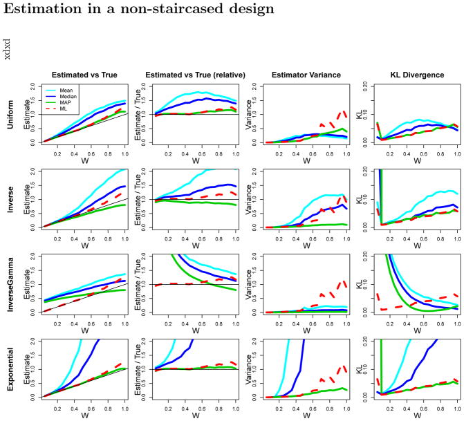
An analog to Figure 3 using a design in which all subjects see all items, from (1, 2) up to (12, 13) (i.e. not a staircased design). This shows similar patterns of performance for the various estimation schemes, indicating that the superiority of an estimator with an inverse prior is not an artifact of the staircased design.

Figure 6.

An analog to Figure 3 in the situation where subjects make mistakes 10% of the time, independent of the displayed stimuli (for instance, through inattention). This demonstrates that the efficient performance of the inverse prior holds even when the fit model is somewhat misspecified in that it neglects the extra noise. Note that in this case, the estimators tend to over-estimate W since the additional noise leads them to conclude that W is worse (higher) than it truly is.