Metainference: A Bayesian inference method for heterogeneous systems

Researchers present a Bayesian inference method for heterogeneous systems that integrates prior information with noisy experimental data.

Abstract

Modeling a complex system is almost invariably a challenging task. The incorporation of experimental observations can be used to improve the quality of a model and thus to obtain better predictions about the behavior of the corresponding system. This approach, however, is affected by a variety of different errors, especially when a system simultaneously populates an ensemble of different states and experimental data are measured as averages over such states. To address this problem, we present a Bayesian inference method, called “metainference,” that is able to deal with errors in experimental measurements and with experimental measurements averaged over multiple states. To achieve this goal, metainference models a finite sample of the distribution of models using a replica approach, in the spirit of the replica-averaging modeling based on the maximum entropy principle. To illustrate the method, we present its application to a heterogeneous model system and to the determination of an ensemble of structures corresponding to the thermal fluctuations of a protein molecule. Metainference thus provides an approach to modeling complex systems with heterogeneous components and interconverting between different states by taking into account all possible sources of errors.

INTRODUCTION

The quantitative interpretation of experimental measurements requires the construction of a model of the system under observation. The model usually consists of a description of the system in terms of several parameters, which are determined by requiring consistency with the experimental measurements themselves and with theoretical information, either physical or statistical in nature. This procedure presents several complications. First, experimental data (Fig. 1A) are always affected by random and systematic errors (Fig. 1B, green), which must be properly accounted for to obtain accurate and precise models. Furthermore, when integrating multiple experimental observations, one must consider that each experiment has a different level of noise so that every element of information is properly weighted according to its reliability. Second, the prediction of experimental observables from the model, which is required to assess the consistency, is often based on an approximate description of a given experiment (the so-called “forward model”) and thus is intrinsically inaccurate in itself (Fig. 1B, green). Third, physical systems under equilibrium conditions often populate a variety of different states whose thermodynamic behavior can be described by statistical mechanics. In these heterogeneous systems, experimental observations depend on—and thus probe—a population of states (Fig. 1B, purple) so that one should determine an ensemble of models rather than a single one (Fig. 1C).

Fig. 1. Schematic illustration of the metainference method.

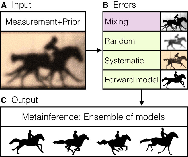
(A and B) To generate accurate and precise models from input information (A), one must recognize that data from experimental measurements are always affected by random and systematic errors and that the theoretical interpretation of an experiment may also be inaccurate (B; green). Moreover, data collected on heterogeneous systems depend on a multitude of states and their populations (B; purple). (C) Metainference can treat all of these sources of error and thus it can properly combine multiple experimental data with prior knowledge of a system to produce ensembles of models consistent with the input information.

Among the theoretical approaches available for model building, two frameworks have emerged as particularly successful: Bayesian inference (1–3) and the maximum entropy principle (4). Bayesian modeling is a rigorous approach to combining prior information on a system with experimental data and to dealing with errors in such data (1–3, 5–8). It proceeds by constructing a model of noise as a function of one or more unknown uncertainty parameters, which quantify the agreement between predictions and observations and which are inferred along with the model of the system. This method has a long history and is routinely used in a wide range of applications, including the reconstruction of phylogenetic trees (9), determination of population structures from genotype data (10), interpolation of noisy data (11), image reconstruction (12), decision theory (13), analysis of microarray data (14), and structure determination of proteins (15, 16) and protein complexes (17). It has also been extended to deal with mixtures of states (18–21) by treating the number of states as a parameter to be determined by the procedure. The maximum entropy principle is at the basis of approaches that deal with experimental data averaged over an ensemble of states (4) and provides a link between information theory and statistical mechanics. In these methods, an ensemble generated using a prior model is minimally modified by some partial and inaccurate information to exactly match the observed data. In the recently proposed replica-averaging scheme (22–26), this result is achieved by modeling an ensemble of replicas of the system using the available information and additional terms that restrain the average values of the predicted data to be close to the experimental observations. This method has been used to determine ensembles representing the structure and dynamics of proteins (22–26).

Each of the two methods described above can deal with some, but not all, of the challenges in characterizing complex systems by integrating multiple sources of information (Fig. 1B). To simultaneously overcome all of these problems, we present the “metainference” method, a Bayesian inference approach that quantifies the extent to which a prior distribution of models is modified by the introduction of experimental data that are expectation values over a heterogeneous distribution and subject to errors. To achieve this goal, metainference models a finite sample of this distribution, in the spirit of the replica-averaged modeling based on the maximum entropy principle. Notably, our approach reduces to the maximum entropy modeling in the limit of the absence of noise in the data, and to standard Bayesian modeling when experimental data are not ensemble averages. This link between Bayesian inference and the maximum entropy principle is not surprising given the connections between these two approaches (27, 28). We first benchmark the accuracy of our method on a simple heterogeneous model system, in which synthetic experimental data can be generated with different levels of noise as averages over a discrete number of states of the system. We then show its application with nuclear magnetic resonance (NMR) spectroscopy data in the case of the structural fluctuations of the protein ubiquitin in its native state, which we modeled by combining chemical shifts with residual dipolar couplings (RDCs).

RESULTS AND DISCUSSION

Metainference is a Bayesian approach to modeling a heterogeneous system and all sources of error by considering a set of copies of the system (replicas), which represent a finite sample of the distribution of models, in the spirit of the replica-averaged formulation of the maximum entropy principle (22–26). The generation of models by suitable sampling algorithms [typically Monte Carlo or molecular dynamics (MD)] is guided by a score given in terms of the negative logarithm of the posterior probability (Materials and Methods) 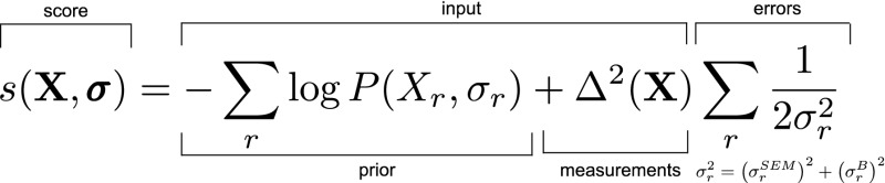where X = [X_r] and σ = [σ_r] are, respectively, the sets of conformational states and uncertainties, one for each replica. σ_r includes all of the sources of errors, that is, the error in representing the ensemble with a finite number of replicas (${\mathrm{\sigma }}_{\mathit{r}}^{\text{SEM}}$), as well as random, systematic, and forward model errors (${\mathrm{\sigma }}_{\mathit{r}}^{\mathrm{B}}$). P is the prior probability that encodes information other than experimental data, and Δ²(X) is the deviation of the experimental data from the data predicted by the forward model. This schematic equation, which omits the data likelihood normalization term for the uncertainty parameters, holds for Gaussian errors and a single data point, and a more general formulation can be found in Materials and Methods (Eqs. 5 and 8).

Metainference of a heterogeneous model system

We first illustrate the metainference method for a model system that can simultaneously populate a set of discrete states, that is, a mixture. In this example, the number of states in the mixture and their population can be varied arbitrarily. We created synthetic data as ensemble averages over these discrete states (Fig. 2A), and we added random and systematic noise. We thus introduced prior information, which provides an approximate description of the system and its distribution of states and whose accuracy can also be tuned. We then used the reference data to complement the prior information and to recover the correct number and populations of the states. We tested the following approaches: metainference (with the Gaussian and outliers noise models in Eqs. 9 and 11, respectively), replica-averaging maximum entropy, and standard Bayesian inference (that is, Bayesian inference without mixtures). The accuracy of a given approach was defined as the root mean square deviation of the inferred populations from the correct populations of the discrete states. We benchmarked the accuracy as a function of the number of data points used, the level of noise in the data, the number of states and replicas, and the accuracy of the prior information. Details of the simulations, generation of data, sampling algorithm, and likelihood and model to treat systematic errors and outliers can be found in the Supplementary Materials.

Fig. 2. Metainference of a model heterogeneous system.

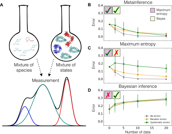
(A) Equilibrium measurements on mixtures of different species or states do not reflect a single species or conformation but are instead averaged over the whole ensemble. (B to D) We describe such a scenario using a model heterogeneous system composed of multiple discrete states on which we tested metainference (B), the maximum entropy approach (C), and standard Bayesian modeling (D), using synthetic data. We assess the accuracy of these methods in determining the populations of the states as a function of the number of data points used and the level of noise in the data. Among these approaches, metainference is the only one that can deal with both heterogeneity and errors in the data; the maximum entropy approach can treat only the former, whereas standard Bayesian modeling can treat only the latter.

Comparison with the maximum entropy method

We found that the metainference and maximum entropy methods perform equally well in the absence of noise in the data or in the presence of random noise alone (Fig. 2, B and C, gray and orange lines), as expected, given that maximum entropy is particularly effective in the case of mixtures of states (22, 23). The accuracy of the two methods was comparable and, most importantly, increased with the number of data points used (Fig. 2, B and C). With 20 data points and 128 replicas, and in the absence of noise, the accuracy averaged over 300 independent simulations of a five-state system was equal to 0.4 ± 0.2% and 0.2 ± 0.1% for the metainference and maximum entropy approaches, respectively. For reference, the accuracy of the prior information alone was much lower, that is, 16%. Metainference, however, outperformed the maximum entropy approach in the presence of systematic errors (Fig. 2, B and C, green lines). The accuracy of metainference increased significantly more rapidly upon the addition of new information, despite the high level of noise. When using 20 data points, 128 replicas, and 30% outliers ratio, the accuracy averaged over 300 independent simulations of a five-state system was equal to 2 ± 2% and 14 ± 5% for the metainference and maximum entropy approaches, respectively. As systematic errors are ubiquitous both in the experimental data and in the forward model used to predict the data, this situation more closely reflects a realistic scenario. The ability of metainference to effectively deal with averaging and with the presence of systematic errors at the same time is the main motivation for introducing this method. This approach can thus leverage the substantial amount of noisy data produced by high-throughput techniques and accurately model conformational ensembles of heterogeneous systems.

Comparison with standard Bayesian modeling

In the standard Bayesian approach, one assumes the presence of a single state in the sample and estimates its probability or confidence level given experimental data and prior knowledge available. When modeling multiple-state systems with ensemble-averaged data and standard Bayesian modeling, one could be tempted to interpret the probability of each state as its equilibrium population. In doing so, however, one makes a significant error, which grows with the number of data points used, regardless of the level of noise in the data (Fig. 2D).

Role of prior information

We tested two priors of different accuracies, with an average population error per state equal to 8 and 16%, respectively. The results suggest that the number of experimental data points required to achieve a given accuracy of the inferred populations depends on the quality of the prior information (fig. S1). The more accurate the prior is, the fewer data points are needed. This is an intuitive, yet important, result. Accurate priors almost invariably require more complex descriptions of the system under study; thus, they usually come at a higher computational cost.

Scaling with the number of replicas

As the number of replicas grows, the error in estimating ensemble averages using a finite number of replicas decreases, and the overall accuracy of the inferred populations increases (fig. S2), regardless of the level of noise in the data. Furthermore, we verified numerically that, in the absence of random and systematic errors in the data, the intensity of the harmonic restraint, which couples the average of the forward model on the N replicas to the experimental data (Eq. 7), scales as N² (Fig. 3). This test confirms that, in the limit of the absence of noise in the data, metainference coincides with the replica-averaging maximum entropy modeling (Materials and Methods).

Fig. 3. Scaling of the metainference harmonic restraint intensity in the absence of noise in the data.

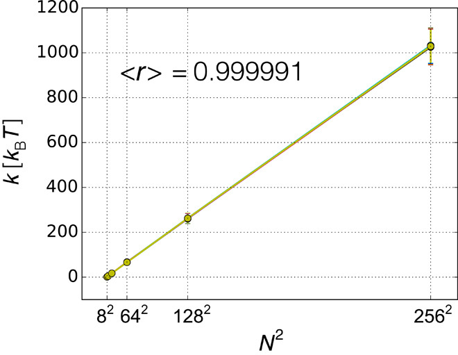
We verified numerically that in the absence of noise in the data and with a Gaussian noise model, the intensity of the metainference harmonic restraint $\mathit{k}={\displaystyle \sum _{\mathit{r}=1}^{\mathit{N}}}\frac{1}{{\mathrm{\sigma }}_{\mathit{r}}^2}$, which couples the average of the forward model over the N replicas to the experimental data point (Eq. 7), scales as N². This test was carried out in the model system at five discrete states, with 20 data points and with the prior at 16% accuracy. For each of the 20 data points, we report the average restraint intensity over the entire Monte Carlo simulation and its SD when using 8, 16, 32, 64, 128, and 256 replicas. The average Pearson’s correlation coefficient on the 20 data points is 0.999991 ± 3 × 10⁻⁶, showing that metainference coincides with the replica-averaging maximum entropy modeling in the limit of the absence of noise in the data.

Scaling with the number of states

Metainference is also robust to the number of states populated by the system. We tested our model in the case of 5 and 50 states and determined that the number of data points needed to achieve a given accuracy scales less than linearly with the number of states (fig. S3).

Outliers model and error marginalization

As the numbers of data points and replicas increase, using one error parameter per replica and data point becomes computationally more and more inconvenient. In this situation, one can assume a unimodal and long-tailed distribution for the errors, peaked around a typical value for a data set (or experiment type) and replica, and marginalize all of the uncertainty parameters of the single data points (Materials and Methods). The accuracy of this marginalized error model was found to be similar to the case in which a single error parameter was used for each data point (fig. S4).

Analysis of the inferred uncertainties

We analyzed the distribution of inferred uncertainties σ^B in the presence of systematic errors (outliers) when using a Gaussian data likelihood with one uncertainty per data point (Eq. 9) and the outliers model with one uncertainty per data set (Eq. 11). In the former case, metainference was able to automatically detect the data points affected by systematic errors, assign a higher uncertainty unto them, and thus downweight the associated restraints (Fig. 4A). In the latter case, the inferred typical data set uncertainty was somewhere in between the uncertainty inferred using the Gaussian likelihood on the data points with no noise and the uncertainty inferred using the Gaussian likelihood on the outliers (Fig. 4B). In this specific test (five states, 20 data points including eight outliers, prior accuracy equal to 16%, and 128 replicas), both data noise models generated an ensemble of comparable accuracy (3%).

Fig. 4. Analysis of the inferred uncertainties.

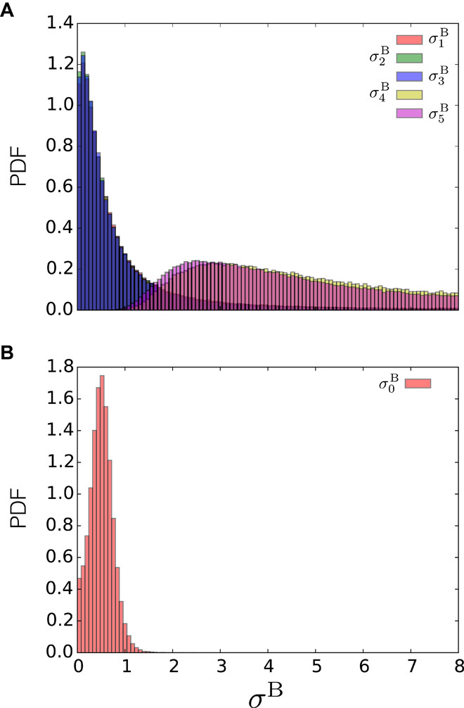
(A and B) Distributions of inferred uncertainties (PDF) in the presence of systematic errors, using (A) a Gaussian data likelihood with one uncertainty per data point and (B) the outliers model with one uncertainty per data set. This test was carried out in the model system at five discrete states, with 20 data points (of which eight were outliers), 128 replicas, and the prior at 16% accuracy. For the Gaussian noise model, we report the distributions of three representative points not affected by noise (${\mathrm{\sigma }}_{1-3}^{\mathrm{B}}$) and of two representative points affected by systematic errors (${\mathrm{\sigma }}_4^{\mathrm{B}}$ and ${\mathrm{\sigma }}_5^{\mathrm{B}}$). For the outliers model, we report the distribution of the typical data set uncertainty (${\mathrm{\sigma }}_0^{\mathrm{B}}$).

Metainference in integrative structural biology

We compared the metainference and maximum entropy approaches using NMR experimental data on a classical example in structural biology—the structural fluctuations in the native state of ubiquitin (22, 29, 30). A conformational ensemble of ubiquitin was modeled using CA, CB, CO, HA, HN, and NH chemical shifts combined with RDCs collected in a steric medium (30) (Fig. 5A). The ensemble was validated by multiple criteria (table S1). The stereochemical quality was assessed by PROCHECK (31); data not used for modeling, including ³J_HNC and ³J_HNHA scalar couplings and RDCs collected in other media (32), were backcalculated and compared with the experimental data. Exhaustive sampling was achieved by 1-μs-long MD simulations performed with GROMACS (33) equipped with PLUMED (34). We used the CHARMM22* force field as prior information (35). Additional details of these simulations can be found in the Supplementary Materials.

Fig. 5. Example of the application of metainference in integrative structural biology.

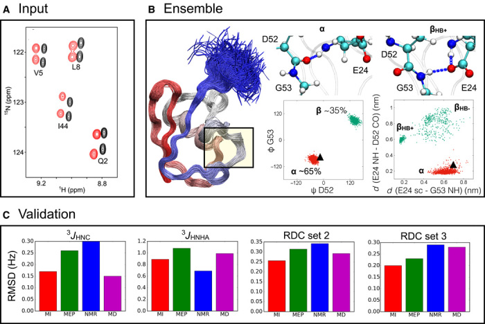
(A) Comparison of the metainference and maximum entropy approaches by modeling the structural fluctuations of the protein ubiquitin in its native state using NMR chemical shifts and RDC data. (B) The metainference ensemble supports the finding (36) that a major source of dynamics involves a flip of the backbone of residues D⁵²-G⁵³ (B; left scatterplot), which interconverts between an α state with a 65% population and a β state with a 35% population. This flip is coupled with the formation of a hydrogen bond between the side chain of E²⁴ and the backbone of G⁵³ (B; right scatterplot); the state in which the hydrogen bond is present (β_HB+) is populated 30% of the time, and the state in which the hydrogen bond is absent (β_HB−) is populated 5% of the time. By contrast, the NMR structure (Protein Data Bank code 1D3Z) provides a static picture of ubiquitin in this region in which the α state is the only populated one (black triangle). (C) Validation of the metainference (MI; red) and maximum entropy principle (MEP; green) ensembles, along with the NMR structure (blue) and the MD ensemble (purple), by the backcalculation of experimental data not used in the modeling: ³J_HNC and ³J_HNHA scalar couplings and two independent sets of RDCs (RDC sets 2 and 3).

The quality of the metainference ensemble (Fig. 5B) was higher than that of the maximum entropy ensemble, as suggested by the better fit with the data not used in the modeling (Fig. 5C and table S1) and by the stereochemical quality (table S2). Data used as restraints were also more accurately reproduced by metainference. One of the major differences between the two approaches is that metainference can deal more effectively with the errors in the chemical shifts calculated on different nuclei. The more inaccurate HN and NH chemical shifts were detected by metainference and thus automatically downweighted in constructing the ensemble (Fig. 6).

Fig. 6. Distributions (PDF) of restraint intensities for different chemical shifts of ubiquitin.

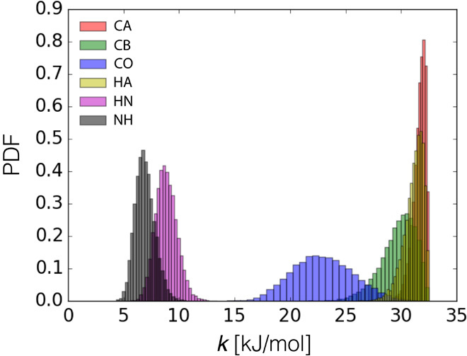
When combining data from different experiments, metainference automatically determines the weight of each piece of information. In the case of ubiquitin, the NH and HN chemical shifts were determined as the less reliable data and thus were downweighted in the construction of the ensemble of models. From this procedure it is not possible to determine whether these two specific data sets have a higher level of random or systematic noise, or whether instead the CAMSHIFT predictor (38) is less accurate for these specific nuclei.

We also compared the metainference ensemble with an ensemble generated by standard MD simulations and with a high-resolution NMR structure. The metainference ensemble obtained by combining chemical shifts and RDCs reproduced all of the experimental data not used for the modeling better than the MD ensemble and the NMR structure. The only exception were the ³J_HNC scalar couplings, which were slightly more accurate in the MD ensemble, and the ³J_HNHA scalar couplings, which were better predicted by the NMR structure (Fig. 5C and table S1).

The NMR structure, which was determined according to the criterion of maximum parsimony, accurately reproduced most of the available experimental data. Ubiquitin, however, exhibits rich dynamical properties over a wide range of time scales averaged in the experimental data (36). In particular, a main source of dynamics involves a flip of the backbone of residues D⁵²-G⁵³ coupled with the formation of a hydrogen bond between the side chain of E²⁴ and the backbone of G⁵³. Although metainference was able to capture the conformational exchange between these two states, the static representation provided by the NMR structure could not (Fig. 5B).

In conclusion, we have presented the metainference approach, which enables the building of an ensemble of models consistent with experimental data when the data are affected by errors and are averaged over mixtures of the states of a system. Because complex systems and experimental data almost invariably exhibit both heterogeneity and errors, we anticipate that our method will find applications across a wide variety of scientific fields, including genomics, proteomics, metabolomics, and integrative structural biology.

MATERIALS AND METHODS

The quantitative understanding of a system involves the construction of a model M to represent it. If a system can occupy multiple possible states, one should determine the distribution of models p(M) that specifies in which states the system can be found and the corresponding probabilities. To construct this distribution of models, one should take into account the consistency with the overall knowledge that one has about the system. This includes theoretical knowledge (called the “prior” information I) and the information acquired from experimental measurements (that is, the “data” D) (1). In Bayesian inference, the probability of a model given the information available is known as the posterior probability p(M|D, I) of M given D and I, and it is given by

$$\mathit{p}(\mathit{M}|\mathit{D},\mathit{I})\propto \mathit{p}(\mathit{D}|\mathit{M},\mathit{I})\mathit{p}(\mathit{M}|\mathit{I})$$ (1)

where the likelihood function p(D|M, I) is the probability of observing D given M and I, and the prior probability p(M|I) is the probability of M given I. To define the likelihood function, one needs a forward model f(M) that predicts the data that would be observed for model M and a noise model that specifies the distribution of the deviations between the observed data and the predicted data. In the following, we assumed that the forward model depends only on the conformational state X of the system and that the noise model is defined in terms of unknown parameters σ that are part of the model M = (X, σ). These parameters quantify the level of noise in the data, and they are inferred along with the state X by sampling the posterior distribution. The sampling is usually carried out using computational techniques such as Monte Carlo, MD, or combined methods based on Gibbs sampling (1).

Mixture of states

Experimental data collected under equilibrium conditions are usually the result of ensemble averages over a large number of states. In metainference, the prior information p(X) of state X provides an a priori description of the distribution of states. To quantify the fit with the observed data and to determine to what extent the prior distribution is modified by the introduction of the data, we needed to calculate the expectation values of the forward model over the distribution of states. Inspired by the replica-averaged modeling based on the maximum entropy principle (22–26), we considered a finite sample of this distribution by simultaneously modeling N replicas of the model M = [M_r], and we calculated the forward model as an average over the states X = [X_r]

$$\mathit{f}(\mathbf{X})=\frac{1}{\mathit{N}}{\displaystyle \sum _{\mathit{r}=1}^{\mathit{N}}}\mathit{f}({\mathit{X}}_{\mathit{r}})$$ (2)

Typically, we have information only about expectation values on the distribution of states X, and not on the other parameters of the model, such as σ. However, we were also interested in determining how the prior distributions of these parameters are modified by the introduction of the experimental data. Therefore, we modeled a finite sample of the joint probability distribution of all parameters of the model.

For a reduced computational cost, a relatively small number of replicas are typically used in the modeling. In this situation, the estimate f(X) of the forward model deviated from the average $\tilde{\mathit{f}}$ that would be obtained using an infinite number of replicas. This was an unknown quantity, which we added to the parameters of our model. However, the central limit theorem provided a strong parametric prior because it guaranteed that the probability of having a certain value of $\tilde{\mathit{f}}$ given a finite number of states X is a Gaussian distribution

$$\mathit{p}(\tilde{\mathit{f}}|\mathbf{X},{\mathrm{\sigma }}^{\text{SEM}})=\frac{1}{\sqrt{2\mathrm{\pi }}{\mathrm{\sigma }}^{\text{SEM}}}\text{exp}[-\frac{{(\tilde{\mathit{f}}-\mathit{f}(\mathbf{X}))}^2}{2{({\mathrm{\sigma }}^{\text{SEM}})}^2}]$$ (3)

where the standard error of the mean σ^SEM decreases with the square root of the number of replicas

$${\mathrm{\sigma }}^{\text{SEM}}\propto \frac{1}{\sqrt{\mathit{N}}}$$ (4)

We recognized that, in considering a finite sample of our distribution of states, we introduced an error in the calculation of expectation values. Therefore, experimental data should be compared to the (unknown) average of the forward model over an infinite number of replicas $\tilde{\mathit{f}}$, which is then related to the average over our finite sample f(X) via the central limit theorem of Eq. 3. From these considerations, we can derive the posterior probability of the ensemble of N replicas representing a finite sample of our distribution of models $\mathbf{M}=(\mathbf{X},\tilde{\mathit{f}},{\mathbf{\sigma }}^{\mathbf{B}},{\mathbf{\sigma }}^{\mathbf{S}\mathbf{E}\mathbf{M}})$. In the case of a single experimental data point d, this can be expressed as (Supplementary Materials)

$$\mathit{p}(\mathbf{X},\tilde{\mathit{f}},{\mathbf{\sigma }}^{\mathbf{B}},{\mathbf{\sigma }}^{\mathbf{S}\mathbf{E}\mathbf{M}}|\mathit{d},\mathit{I})\propto {\displaystyle \prod _{\mathit{r}=1}^{\mathit{N}}}\mathit{p}(\mathit{d}|{\tilde{\mathit{f}}}_{\mathit{r}},{\mathrm{\sigma }}_{\mathit{r}}^{\mathrm{B}})\mathit{p}({\tilde{\mathit{f}}}_{\mathit{r}}|\mathbf{X},{\mathrm{\sigma }}_{\mathit{r}}^{\text{SEM}})\mathit{p}({\mathrm{\sigma }}_{\mathit{r}}^{\mathrm{B}})\mathit{p}({\mathit{X}}_{\mathit{r}})\mathit{p}({\mathrm{\sigma }}_{\mathit{r}}^{\text{SEM}})$$ (5)

The data likelihood $\mathit{p}(\mathit{d}|{\tilde{\mathit{f}}}_{\mathit{r}},{\mathrm{\sigma }}_{\mathit{r}}^{\mathrm{B}})$ relates the experimental data d to the average of the forward model over an infinite number of replicas, given the uncertainty ${\mathrm{\sigma }}_{\mathit{r}}^{\mathrm{B}}$. This parameter describes random and systematic errors in the experimental data and errors in the forward model. The functional form of $\mathit{p}(\mathit{d}|{\tilde{\mathit{f}}}_{\mathit{r}},{\mathrm{\sigma }}_{\mathit{r}}^{\mathrm{B}})$ depends on the nature of the experimental data, and it is typically a Gaussian or lognormal distribution. As noted above, $\mathit{p}({\tilde{\mathit{f}}}_{\mathit{r}}|\mathbf{X},{\mathrm{\sigma }}_{\mathit{r}}^{\text{SEM}})$ is the parametric prior on ${\tilde{\mathit{f}}}_{\mathit{r}}$ that relates the (unknown) average ${\tilde{\mathit{f}}}_{\mathit{r}}$ to the estimate f(X) computed with a finite number of replicas N via the central limit theorem of Eq. 3, and thus it is always a Gaussian distribution. $\mathit{p}({\mathrm{\sigma }}_{\mathit{r}}^{\text{SEM}})$ is the prior on the standard error of the mean ${\mathrm{\sigma }}_{\mathit{r}}^{\text{SEM}}$ and encodes Eq. 4. $\mathit{p}({\mathrm{\sigma }}_{\mathit{r}}^{\mathrm{B}})$ is the prior on the uncertainty parameter ${\mathrm{\sigma }}_{\mathit{r}}^{\mathrm{B}}$, and p(X_r) is the prior on the structure X_r.

Gaussian noise model

We can further simplify Eq. 5 in the case of Gaussian data likelihood $\mathit{p}(\mathit{d}|{\tilde{\mathit{f}}}_{\mathit{r}},{\mathrm{\sigma }}_{\mathit{r}}^{\mathrm{B}})$. In this situation, ${\tilde{\mathit{f}}}_{\mathit{r}}$ can be marginalized (Supplementary Materials), and the posterior probability can be written as

$$\mathit{p}(\mathbf{X},\mathbf{\sigma }|\mathit{d},\mathit{I})\propto {\displaystyle \prod _{\mathit{r}=1}^{\mathit{N}}}\frac{1}{\sqrt{2\mathrm{\pi }}{\mathrm{\sigma }}_{\mathit{r}}}\text{exp}[-\frac{{(\mathit{d}-\mathit{f}(\mathbf{X}))}^2}{2{\mathrm{\sigma }}_{\mathit{r}}^2}]\mathit{p}({\mathrm{\sigma }}_{\mathit{r}})\mathit{p}({\mathit{X}}_{\mathit{r}})$$ (6)

where the effective uncertainty ${\mathrm{\sigma }}_{\mathit{r}}=\sqrt{{({\mathrm{\sigma }}_{\mathit{r}}^{\text{SEM}})}^2+{({\mathrm{\sigma }}_{\mathit{r}}^{\mathrm{B}})}^2}$ encodes all sources of errors: the statistical error due to the use of a finite number of replicas, experimental and systematic errors, and errors in the forward model. The associated energy function in units of k_BT becomes

$$\mathit{E}={(\mathit{d}-\mathit{f}(\mathbf{X}))}^2{\displaystyle \sum _{\mathit{r}=1}^{\mathit{N}}}\frac{1}{2{\mathrm{\sigma }}_{\mathit{r}}^2}+{\displaystyle \sum _{\mathit{r}=1}^{\mathit{N}}}[\text{log} {\mathrm{\sigma }}_{\mathit{r}}- \text{log} \mathit{p}({\mathrm{\sigma }}_{\mathit{r}})- \text{log} \mathit{p}({\mathit{X}}_{\mathit{r}})]$$ (7)

This equation shows how metainference includes different existing modeling methods in limiting cases. In the absence of data and forward model errors (${\mathrm{\sigma }}_{\mathit{r}}^{\mathrm{B}}=0$), our approach reduces to the replica-averaged maximum entropy modeling, in which a harmonic restraint couples the replica-averaged observable to the experimental data. The intensity of the restraint $\mathit{k}={\displaystyle \sum _{\mathit{r}=1}^{\mathit{N}}}\frac{1}{{\mathrm{\sigma }}_{\mathit{r}}^2}$ scales with the number of replicas as N², that is, more than linearly, as required by the maximum entropy principle (24). We numerically verified this behavior in our heterogeneous model system in the absence of any errors in the data (Fig. 3). In the presence of errors (${\mathrm{\sigma }}_{\mathit{r}}^{\mathrm{B}}\ne 0$), the intensity k scales as N, and it is modulated by the data uncertainty ${\mathrm{\sigma }}_{\mathit{r}}^{\mathrm{B}}$. Finally, in the case in which the experimental data are not ensemble averages (${\mathrm{\sigma }}_{\mathit{r}}^{\text{SEM}}=0$), we recover the standard Bayesian modeling.

Multiple experimental data points

Equation 5 can be extended to the case of N_d independent data points D = [d_i], possibly gathered in different experiments at varying levels of noise (Supplementary Materials)

$$\mathit{p}(\mathbf{X},\tilde{\mathit{f}},{\mathbf{\sigma }}^{\mathbf{B}},{\mathbf{\sigma }}^{\mathbf{S}\mathbf{E}\mathbf{M}}|\mathbf{D},\mathit{I})\propto {\displaystyle \prod _{\mathit{r}=1}^{\mathit{N}}}{\displaystyle \prod _{\mathit{i}=1}^{{\mathit{N}}_{\mathit{d}}}}\mathit{p}({\mathit{d}}_{\mathit{i}}|{\tilde{\mathit{f}}}_{\mathit{r},\mathit{i}},{\mathrm{\sigma }}_{\mathit{r},\mathit{i}}^{\mathrm{B}})\mathit{p}({\tilde{\mathit{f}}}_{\mathit{r},\mathit{i}}|\mathbf{X},{\mathrm{\sigma }}_{\mathit{r},\mathit{i}}^{\text{SEM}})\mathit{p}({\mathrm{\sigma }}_{\mathit{r},\mathit{i}}^{\mathrm{B}})\mathit{p}({\mathrm{\sigma }}_{\mathit{r},\mathit{i}}^{\text{SEM}}){\displaystyle \prod _{\mathit{r}=1}^{\mathit{N}}}\mathit{p}({\mathit{X}}_{\mathit{r}})$$ (8)

Outliers model

To reduce the number of parameters that need to be sampled in the case of multiple experimental data points, one can model the distribution of the errors around a typical data set error and marginalize the error parameters for the individual data points. For example, a data set can be defined as a set of chemical shifts or RDCs on a given nucleus. In this case, it is reasonable to assume that the level of error of the individual data points in the data set is homogeneous, except for the presence of few outliers. Let us consider, for example, the case of Gaussian data noise. In the case of multiple experimental data points, Eq. 6 becomes

$$\mathit{p}(\mathbf{X},\mathrm{\sigma }|\mathbf{D},\mathit{I})\propto {\displaystyle \prod _{\mathit{r}=1}^{\mathit{N}}}\mathit{p}({\mathit{X}}_{\mathit{r}}){\displaystyle \prod _{\mathit{i}=1}^{{\mathit{N}}_{\mathit{d}}}}\frac{1}{\sqrt{2\mathrm{\pi }}{\mathrm{\sigma }}_{\mathit{r},\mathit{i}}}\text{exp}[-\frac{{({\mathit{d}}_{\mathit{i}}-{\mathit{f}}_{\mathit{i}}(\mathbf{X}))}^2}{2{\mathrm{\sigma }}_{\mathit{r},\mathit{i}}^2}]\mathit{p}({\mathrm{\sigma }}_{\mathit{r},\mathit{i}})$$ (9)

The prior p(σ_r,i) can be modeled using a unimodal distribution peaked around a typical data set effective uncertainty σ_r,0 and with a long tail to tolerate outliers data points (37)

$$\mathit{p}({\mathrm{\sigma }}_{\mathit{r},\mathit{i}})=\frac{2{\mathrm{\sigma }}_{\mathit{r},0}}{\sqrt{\mathrm{\pi }}{\mathrm{\sigma }}_{\mathit{r},\mathit{i}}^2}\text{exp}(-\frac{{\mathrm{\sigma }}_{\mathit{r},0}^2}{{\mathrm{\sigma }}_{\mathit{r},\mathit{i}}^2})$$ (10)

where ${\mathrm{\sigma }}_{\mathit{r},0}=\sqrt{{({\mathrm{\sigma }}^{\text{SEM}})}^2+{({\mathrm{\sigma }}_{\mathit{r},0}^{\mathrm{B}})}^2}$, with σ^SEM as the standard error of the mean for all data points in the data set and replicas and with ${\mathrm{\sigma }}_{\mathit{r},0}^{\mathrm{B}}$ as the typical data uncertainty of the data set. We can thus marginalize σ_r,i by integrating over all its possible values, given that all of the data uncertainties ${\mathrm{\sigma }}_{\mathit{r},\mathit{i}}^{\mathrm{B}}$ range from 0 to infinity

$$\mathit{p}(\mathbf{X},{\mathbf{\sigma }}_{\mathbf{0}}|\mathbf{D},\mathit{I})\propto {\displaystyle \prod _{\mathit{r}=1}^{\mathit{N}}}\mathit{p}({\mathit{X}}_{\mathit{r}}){\displaystyle \prod _{\mathit{i}=1}^{{\mathit{N}}_{\mathit{d}}}}{\displaystyle \underset{{\mathrm{\sigma }}^{\text{SEM}}}{\overset{+\infty }{\int }}}\mathit{d}{\mathrm{\sigma }}_{\mathit{r},\mathit{i}}\frac{\sqrt{2}{\mathrm{\sigma }}_{\mathit{r},0}}{\mathrm{\pi }{\mathrm{\sigma }}_{\mathit{r},\mathit{i}}^3}\text{exp}[-\frac{0.5{({\mathit{d}}_{\mathit{i}}-{\mathit{f}}_{\mathit{i}}(\mathbf{X}))}^2+{\mathrm{\sigma }}_{\mathit{r},0}^2}{{\mathrm{\sigma }}_{\mathit{r},\mathit{i}}^2}]={\displaystyle \prod _{\mathit{r}=1}^{\mathit{N}}}\mathit{p}({\mathit{X}}_{\mathit{r}}){\displaystyle \prod _{\mathit{i}=1}^{{\mathit{N}}_{\mathit{d}}}}\frac{\sqrt{2}{\mathrm{\sigma }}_{\mathit{r},0}}{\mathrm{\pi }}\frac{1}{{({\mathit{d}}_{\mathit{i}}-{\mathit{f}}_{\mathit{i}}(\mathbf{X}))}^2+2{\mathrm{\sigma }}_{\mathit{r},0}^2}\{1-\text{exp}[-\frac{0.5{({\mathit{d}}_{\mathit{i}}-{\mathit{f}}_{\mathit{i}}(\mathbf{X}))}^2+{\mathrm{\sigma }}_{\mathit{r},0}^2}{{({\mathrm{\sigma }}^{\text{SEM}})}^2}]\}$$ (11)

After marginalization, we are left with just one parameter ${\mathrm{\sigma }}_{\mathit{r},0}^{\mathrm{B}}$ per replica that needs to be sampled.

SUPPLEMENTARY MATERIALS

Supplementary material for this article is available at http://advances.sciencemag.org/cgi/content/full/2/1/e1501177/DC1

Derivation of the basic metainference equations

Details of the model system simulations

Details of the ubiquitin MD simulations

Fig. S1. Effect of prior accuracy on the error of the metainference method.

Fig. S2. Scaling of metainference error with the number of replicas at varying levels of noise in the data.

Fig. S3. Scaling of metainference error with the number of states.

Fig. S4. Accuracy of the outliers model.

Table S1. Comparison of the quality of the ensembles obtained using different modeling approaches in the case of the native state of the protein ubiquitin.

Table S2. Comparison of the stereochemical quality of the ensembles or single models generated by the approaches defined in table S1.

References (39–45)

REFERENCES AND NOTES

- 1.G. E. Box, G. C. Tiao, Bayesian Inference in Statistical Analysis (John Wiley & Sons, New York, 2011), vol. 40. [Google Scholar]
- 2.Bernardo J. M., Smith A. F., Bayesian Theory (John Wiley & Sons, New York, 2009), vol. 405. [Google Scholar]
- 3.P. M. Lee, Bayesian Statistics: An Introduction (John Wiley & Sons, New York, 2012). [Google Scholar]
- 4.Jaynes E. T., Information theory and statistical mechanics. Phys. Rev. 106, 620–630 (1957). [Google Scholar]
- 5.Tavaré S., Balding D. J., Griffiths R. C., Donnelly P., Inferring coalescence times from DNA sequence data. Genetics 145, 505–518 (1997). [DOI] [PMC free article] [PubMed] [Google Scholar]
- 6.Pritchard J. K., Seielstad M. T., Perez-Lezaun A., Feldman M. W., Population growth of human Y chromosomes: A study of Y chromosome microsatellites. Mol. Biol. Evol. 16, 1791–1798 (1999). [DOI] [PubMed] [Google Scholar]
- 7.Poole D., Raftery A. E., Inference for deterministic simulation models: The Bayesian melding approach. J. Am. Stat. Assoc. 95, 1244–1255 (2000). [Google Scholar]
- 8.Kennedy M. C., O’Hagan A., Bayesian calibration of computer models. J. R. Stat. Soc. Ser. B Stat. Methodol. 63, 425–464 (2001). [Google Scholar]
- 9.Huelsenbeck J. P., Ronquist F., MRBAYES: Bayesian inference of phylogenetic trees. Bioinformatics 17, 754–755 (2001). [DOI] [PubMed] [Google Scholar]
- 10.Pritchard J. K., Stephens M., Donnelly P., Inference of population structure using multilocus genotype data. Genetics 155, 945–959 (2000). [DOI] [PMC free article] [PubMed] [Google Scholar]
- 11.MacKay D. J. C., Bayesian interpolation. Neural Comp. 4, 415–447 (1992). [Google Scholar]
- 12.Geman S., Geman D., Stochastic relaxation, Gibbs distributions, and the Bayesian restoration of images. IEEE Trans. Pattern Anal. Mach. Intell. 6, 721–741 (1984). [DOI] [PubMed] [Google Scholar]
- 13.J. O. Berger, Statistical Decision Theory and Bayesian Analysis (Springer Science & Business Media, New York, 2013). [Google Scholar]
- 14.Baldi P., Long A. D., A Bayesian framework for the analysis of microarray expression data: Regularized t-test and statistical inferences of gene changes. Bioinformatics 17, 509–519 (2001). [DOI] [PubMed] [Google Scholar]
- 15.Rieping W., Habeck M., Nilges M., Inferential structure determination. Science 309, 303–306 (2005). [DOI] [PubMed] [Google Scholar]
- 16.MacCallum J. L., Perez A., Dill K. A., Determining protein structures by combining semireliable data with atomistic physical models by Bayesian inference. Proc. Natl. Acad. Sci. U.S.A. 112, 6985–6990 (2015). [DOI] [PMC free article] [PubMed] [Google Scholar]
- 17.Erzberger J. P., Stengel F., Pellarin R., Zhang S., Schaefer T., Aylett C. H. S., Cimermančič P., Boehringer D., Sali A., Aebersold R., Ban N., Molecular architecture of the 40S·eIF1·eIF3 translation initiation complex. Cell 158, 1123–1135 (2014). [DOI] [PMC free article] [PubMed] [Google Scholar]
- 18.Cossio P., Hummer G., Bayesian analysis of individual electron microscopy images: Towards structures of dynamic and heterogeneous biomolecular assemblies. J. Struct. Biol. 184, 427–437 (2013). [DOI] [PMC free article] [PubMed] [Google Scholar]
- 19.Marty M. T., Baldwin A. J., Marklund E. G., Hochberg G. K. A., Benesch J. L. P., Robinson C. V., Bayesian deconvolution of mass and ion mobility spectra: From binary interactions to polydisperse ensembles. Anal. Chem. 87, 4370–4376 (2015). [DOI] [PMC free article] [PubMed] [Google Scholar]
- 20.Molnar K. S., Bonomi M., Pellarin R., Clinthorne G. D., Gonzalez G., Goldberg S. D., Goulian M., Sali A., DeGrado W. F., Cys-scanning disulfide crosslinking and Bayesian modeling probe the transmembrane signaling mechanism of the histidine kinase, PhoQ. Structure 22, 1239–1251 (2014). [DOI] [PMC free article] [PubMed] [Google Scholar]
- 21.Street T. O., Zeng X., Pellarin R., Bonomi M., Sali A., Kelly M. J. S., Chu F., Agard D. A., Elucidating the mechanism of substrate recognition by the bacterial Hsp90 molecular chaperone. J. Mol. Biol. 426, 2393–2404 (2014). [DOI] [PMC free article] [PubMed] [Google Scholar]
- 22.Lindorff-Larsen K., Best R. B., DePristo M. A., Dobson C. M., Vendruscolo M., Simultaneous determination of protein structure and dynamics. Nature 433, 128–132 (2005). [DOI] [PubMed] [Google Scholar]
- 23.Cavalli A., Camilloni C., Vendruscolo M., Molecular dynamics simulations with replica-averaged structural restraints generate structural ensembles according to the maximum entropy principle. J. Chem. Phys. 138, 094112 (2013). [DOI] [PubMed] [Google Scholar]
- 24.Roux B., Weare J., On the statistical equivalence of restrained-ensemble simulations with the maximum entropy method. J. Chem. Phys. 138, 084107 (2013). [DOI] [PMC free article] [PubMed] [Google Scholar]
- 25.Pitera J. W., Chodera J. D., On the use of experimental observations to bias simulated ensembles. J. Chem. Theory Comput. 8, 3445–3451 (2012). [DOI] [PubMed] [Google Scholar]
- 26.Boomsma W., Ferkinghoff-Borg J., Lindorff-Larsen K., Combining experiments and simulations using the maximum entropy principle. PLOS Comput. Biol. 10, e1003406 (2014). [DOI] [PMC free article] [PubMed] [Google Scholar]
- 27.A. Giffin, A. Caticha, Updating probabilities with data and moments. arXiv preprint arXiv:0708.1593 (2007).
- 28.A. Caticha, Entropic inference. arXiv preprint arXiv:1011.0723 (2010).
- 29.Vijay-Kumar S., Bugg C. E., Cook W. J., Structure of ubiquitin refined at 1.8 Å resolution. J. Mol. Biol. 194, 531–544 (1987). [DOI] [PubMed] [Google Scholar]
- 30.Cornilescu G., Marquardt J. L., Ottiger M., Bax A., Validation of protein structure from anisotropic carbonyl chemical shifts in a dilute liquid crystalline phase. J. Am. Chem. Soc. 120, 6836–6837 (1998). [Google Scholar]
- 31.Laskowski R. A., MacArthur M. W., Moss D. S., Thornton J. M., PROCHECK: A program to check the stereochemical quality of protein structures. J. Appl. Crystallogr. 26, 283–291 (1993). [Google Scholar]
- 32.Lange O. F., Lakomek N. A., Farès C., Schröder G. F., Walter K. F., Becker S., Meiler J., Grubmüller H., Griesinger C., de Groot B. L., Recognition dynamics up to microseconds revealed from an RDC-derived ubiquitin ensemble in solution. Science 320, 1471–1475 (2008). [DOI] [PubMed] [Google Scholar]
- 33.Pronk S., Páll S., Schulz R., Larsson P., Bjelkmar P., Apostolov R., Shirts M. R., Smith J. C., Kasson P. M., van der Spoel D., Hess B., Lindahl E., GROMACS 4.5: A high-throughput and highly parallel open source molecular simulation toolkit. Bioinformatics 29, 845–854 (2013). [DOI] [PMC free article] [PubMed] [Google Scholar]
- 34.Tribello G. A., Bonomi M., Branduardi D., Camilloni C., Bussi G., PLUMED 2: New feathers for an old bird. Comput. Phys. Commun. 185, 604–613 (2014). [Google Scholar]
- 35.Piana S., Lindorff-Larsen K., Shaw D. E., How robust are protein folding simulations with respect to force field parameterization? Biophys. J. 100, L47–L49 (2011). [DOI] [PMC free article] [PubMed] [Google Scholar]
- 36.Salvi N., Ulzega S., Ferrage F., Bodenhausen G., Time scales of slow motions in ubiquitin explored by heteronuclear double resonance. J. Am. Chem. Soc. 134, 2481–2484 (2012). [DOI] [PubMed] [Google Scholar]
- 37.D. Sivia, J. Skilling, Data Analysis: A Bayesian Tutorial (Oxford Univ. Press, Oxford, NY, 1996). [Google Scholar]
- 38.Kohlhoff K. J., Robustelli P., Cavalli A., Salvatella X., Vendruscolo M., Fast and accurate predictions of protein NMR chemical shifts from interatomic distances. J. Am. Chem. Soc. 131, 13894–13895 (2009). [DOI] [PubMed] [Google Scholar]
- 39.Jorgensen W. L., Chandrasekhar J., Madura J. D., Impey R. W., Klein M. L., Comparison of simple potential functions for simulating liquid water. J. Chem. Phys. 79, 926–935 (1983). [Google Scholar]
- 40.Hess B., Bekker H., Berendsen H. J., Fraaije J. G., LINCS: A linear constraint solver for molecular simulations. J. Comput. Chem. 18, 1463–1472 (1997). [Google Scholar]
- 41.Bussi G., Donadio D., Parrinello M., Canonical sampling through velocity rescaling. J. Chem. Phys. 126, 014101 (2007). [DOI] [PubMed] [Google Scholar]
- 42.Shen Y., Bax A., SPARTA+: A modest improvement in empirical NMR chemical shift prediction by means of an artificial neural network. J. Biomol. NMR 48, 13–22 (2010). [DOI] [PMC free article] [PubMed] [Google Scholar]
- 43.Zweckstetter M., Bax A., Prediction of sterically induced alignment in a dilute liquid crystalline phase: Aid to protein structure determination by NMR. J. Am. Chem. Soc. 122, 3791–3792 (2000). [Google Scholar]
- 44.Barfield M., Structural dependencies of interresidue scalar coupling h3JNCʹ and donor 1H chemical shifts in the hydrogen bonding regions of proteins. J. Am. Chem. Soc. 124, 4158–4168 (2002). [DOI] [PubMed] [Google Scholar]
- 45.Vögeli B., Ying J., Grishaev A., Bax A., Limits on variations in protein backbone dynamics from precise measurements of scalar couplings. J. Am. Chem. Soc. 129, 9377–9385 (2007). [DOI] [PubMed] [Google Scholar]
Associated Data
This section collects any data citations, data availability statements, or supplementary materials included in this article.