Robust reconstruction of gene expression profiles from reporter gene data using linear inversion

Abstract

Motivation: Time-series observations from reporter gene experiments are commonly used for inferring and analyzing dynamical models of regulatory networks. The robust estimation of promoter activities and protein concentrations from primary data is a difficult problem due to measurement noise and the indirect relation between the measurements and quantities of biological interest.

Results: We propose a general approach based on regularized linear inversion to solve a range of estimation problems in the analysis of reporter gene data, notably the inference of growth rate, promoter activity, and protein concentration profiles. We evaluate the validity of the approach using in silico simulation studies, and observe that the methods are more robust and less biased than indirect approaches usually encountered in the experimental literature based on smoothing and subsequent processing of the primary data. We apply the methods to the analysis of fluorescent reporter gene data acquired in kinetic experiments with Escherichia coli. The methods are capable of reliably reconstructing time-course profiles of growth rate, promoter activity and protein concentration from weak and noisy signals at low population volumes. Moreover, they capture critical features of those profiles, notably rapid changes in gene expression during growth transitions.

Availability and implementation: The methods described in this article are made available as a Python package (LGPL license) and also accessible through a web interface. For more information, see https://team.inria.fr/ibis/wellinverter.

Contact: Hidde.de-Jong@inria.fr

Supplementary information: Supplementary data are available at Bioinformatics online.

1 Introduction

Over the past decade, a variety of new experimental technologies have become available for measuring gene expression over time. They provide valuable information for the construction and validation of models of gene regulatory networks, involving tasks like parameter estimation, hypothesis testing and model selection (Bansal et al., 2007; de Smet and Marchal, 2010; Villaverde and Banga, 2014). A critical step in the exploitation of the experimental data is the estimation of biologically relevant quantities, in particular promoter activities (the rate of transcription of a gene as a fraction of the maximum rate), mRNA concentrations and protein concentrations, from the primary data provided by the measurement instruments. This requires data analysis procedures that are unbiased and robust to measurement noise.

Fluorescent reporter genes have become widely used for monitoring gene expression in bacteria at high temporal resolution in a non-intrusive way (Chudakov et al., 2010; Giepmans et al., 2006). The underlying principle is the fusion of a gene of interest and/or the promoter region driving its expression with a gene encoding a fluorescent protein (Fig. 1). A bacterial strain carrying the resulting reporter gene, on the chromosome or on a plasmid, emits a fluorescence signal proportional to the amount of reporter protein in the cell. When reporter strains are grown in a microplate, the fluorescence and the absorbance (optical density) of the culture can be automatically measured every few minutes in a highly parallelized way. The resulting data contain information on population-level gene expression that is highly valuable for such applications as the inference and analysis of regulatory networks in bacterial cells (Berthoumieux et al., 2013; Gerosa et al., 2013; Keren et al., 2013; Ronen et al., 2002; Stefan et al., 2015).

Fig. 1.

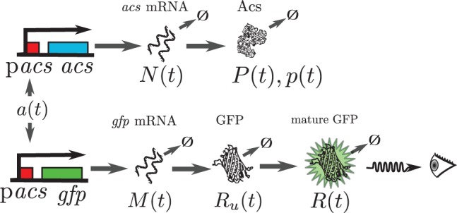
Expression of the gene acs in Escherichia coli and the associated reporter gene pacs-gfp. acs and gfp mRNA are transcribed, and translated into the proteins Acs and GFP, respectively. Both mRNA and protein are degraded. Moreover, GFP is converted into a mature form in which it emits fluorescence when excited. Because acs and its reporter have the same promoter region, the transcriptional regulation of the two genes is identical. The variables are as defined in Equations (16) and (17)

The extraction of useful information from reporter gene data is not easy to achieve though, since it is often buried in noise, especially at low population densities. Moreover, the fluorescence and absorbance measurements are only indirectly related to promoter activities and protein concentrations, requiring dynamical models of the expression of reporter genes for their interpretation. Several methods have been proposed to process the fluorescence and absorbance signals and estimate time-varying promoter activities and protein concentrations from the data (Aïchaoui et al., 2012; Bansal et al., 2012; de Jong et al., 2010; Finkenstädt et al., 2008; Leveau and Lindow, 2001; Lichten et al., 2014; Porreca et al., 2010; Ronen et al., 2002; Wang et al., 2008). The methods differ in the scope of the estimation problems considered, some being restricted to the inference of promoter activities and others also considering mRNA and protein concentrations. In addition, the approaches used to estimate these quantities from the primary data are quite different. Some methods are indirect, in the sense that they smoothen the data first and reconstruct the profiles of interest via the measurement model only in a second step. This results in a propagation of estimation errors that is difficult to control. Other methods state a regularized data fitting problem directly in terms of the quantities of interest, thus, proceeding in a single and better controlled optimization step.

In this article, we propose a general, comprehensive approach toward the reconstruction of gene expression profiles from reporter gene data and solve the estimation problems it comprises in a mathematically sound and practical manner. We formulate the estimation problems in the classical framework of regularized linear inversion (Bertero, 1989; de Nicolao et al., 1997; Wahba, 1990), which gives access to a range of powerful tools for robust estimation. Contrary to the related work of Bansal et al. (2012) and Porreca et al. (2010), we consider not only the inference of promoter activities, but also of growth rates and protein concentrations. Moreover, no restrictions are imposed that limit the practical applicability of the approach. We propose efficient procedures for the implementation of the methods and show by means of an in silico simulation study under realistic conditions that they perform better than the indirect approaches usually encountered in the experimental literature. The algorithms have been implemented in a Python package and are also accessible through a web application.

Our linear inversion methods have been tested on fluorescent reporter gene data acquired in experiments with the model bacterium Escherichia coli. These experiments aim at quantifying the dynamics of gene expression during growth transitions induced by carbon upshift or depletion. We show that linear inversion succeeds in robustly reconstructing growth rate, promoter activity and protein concentration over the entire duration of the experiment, in particular in the beginning when the population density and thus the signal-to-noise ratio are low. Moreover, we show that our methods reliably capture rapid changes in gene expression during growth transitions, when promoter activities may change 10- to 100-fold within a dozen of minutes (Baptist et al., 2013; Enjalbert et al., 2013; Kao et al., 2005). Reconstructing these transient gene expression profiles from the data is highly important for increasing our understanding of the functioning of the underlying regulatory networks, but is difficult to achieve.

To the best of our knowledge, the methods and computer tools presented in this paper provide the most comprehensive solution for analyzing reporter gene data available to date. Although the application has focused on fluorescent reporter gene data, the methods are directly applicable to the analysis of luminescent reporter gene data or other time-series gene expression datasets. In addition, the gene expression models underlying the methods are valid not only for bacteria but also for higher organisms.

2 Linear inversion methods

In this section, we review properties of linear ordinary differential equations (ODEs) and linear relationships between different outputs driven by the same input. This theoretical framework enables us to estimate growth rate, promoter activity and reporter concentration using simple linear inversions in Section 3.

2.1 Inversion of a linear ODE system

We consider the following linear ODE model with input $u(t)\in \mathbb{R}$ and output $y(t)\in \mathbb{R}$:

$$\{\begin{array}{l}\frac{d}{dt}x(t)=A(t)x(t)+B(t)u(t),\\ y(t)=C(t)x(t),\\ x(0)=x_0.\end{array}$$ (1)

In this system, $x(t)\in {\mathbb{R}}^n$ is a vector of state variables, and $A(t),B(t),C(t)$ are known time-varying matrices with dimensions n × n, $n\times 1,1\times n$, respectively. Given a set of noisy observations ${\left(\tilde{y}(t_i)\right)}_{1\le i\le N_y}$ of $y(t_i)$, we wish to estimate the unknown input u(t) and initial conditions $x_0$. The solution of Equation (1) at time t with input u and initial conditions $x_0$ can be formulated explicitly as:

$$y(t,u,x_0)=C(t)\left(\Phi (t,0)x_0+{\displaystyle {\int }_0^t\Phi }(t,\tau )B(\tau )u(\tau )d\tau \right),$$ (2)

where $\Phi (t,\tau )$ is known as the state transition matrix in linear systems theory, and depends on the values of A between τ and t (Chen, 1970). Notice that in this equation $y(t,u,x_0)$ depends linearly on the signal u and the initial conditions $x_0$, making the estimation of these variables from ${\left(\tilde{y}(t_i)\right)}_{1\le i\le N_y}$ a linear inversion problem (Bertero, 1989; de Nicolao et al., 1997; Wahba, 1990).

Under the classical assumption of Gaussian i.i.d. measurement noise, the maximum likelihood solution of this problem can equivalently be written as

$$\text{Find\hspace{0.5em}\hspace{0.5em}\hspace{0.5em}}(\widehat{u},{\widehat{x}}_0)=\underset{(u,x_0)}{\text{argmin}}\text{\hspace{0.5em}\hspace{0.5em}Err}(u,x_0),$$ (3)

where

$$\text{Err}(u,x_0)={\displaystyle \sum _{i=1}^{N_y}{\left(y(t_i,u,x_0)-\tilde{y}(t_i)\right)}^2}.$$

Without further assumptions on u(t) this problem is ill-posed, i.e. there are infinitely many equivalent solutions $\left(\widehat{u}(t),{\widehat{x}}_0\right)$, many of which will be unrealistic from a biological point of view. The problem must therefore be regularized by formulating additional assumptions that lead to a unique, acceptable solution.

To this end, we discretize the time space of the input into N_u intervals $[{\tau }_j,{\tau }_{j+1}[$, of equal length $\delta \tau$. We assume that on this grid of time intervals the input u(t) is sufficiently well approximated by a piecewise-constant input ${\left(u({\tau }_j)\right)}_{1\le j\le N_u}$:

$$u(t)={\displaystyle \sum _{j=1}^{N_u}u}({\tau }_j)1_{[{\tau }_j,{\tau }_{j+1}[}(t).$$ (4)

Because the output y(t) depends linearly on u, the values ${\left(y(t_i,u,x_0)\right)}_{1\le i\le N_y}$ depend linearly on ${\left(u({\tau }_j)\right)}_{1\le j\le N_u}$. If we define the following vectors:

$$u=\left(\begin{array}{c}u({\tau }_1)\\ u({\tau }_2)\\ ⋮\\ u({\tau }_{N_u})\end{array}\right),y=\left(\begin{array}{c}y(t_1,u,x_0)\\ y(t_2,u,x_0)\\ ⋮\\ y(t_{N_y},u,x_0)\end{array}\right),\tilde{y}=\left(\begin{array}{c}\tilde{y}(t_1)\\ \tilde{y}(t_2)\\ ⋮\\ \tilde{y}(t_{N_y})\end{array}\right),$$

and $w={\left(\begin{array}{cc}{x}_0& u\end{array}\right)}^T$, then there exists an observation matrix $H_w$ with dimension $(N_u+n)\times N_y$, such that

$$H_{w}w=y.$$ (5)

The matrix $H_w$ is composed of two matrices:

$$H_w=\left(\begin{array}{cc}{H}_{x_0}& H_u\end{array}\right),$$

where $H_{x_0}$ is a $N_y\times n$ matrix describing the influence of the initial conditions on $y$, and $H_u$ a $N_y\times N_u$ matrix describing the influence of $u$ on $y$. The computation of $H_w$ can be generally performed using a numerical ODE solver, as explained in Supplementary Section S3. However, for the cases of interest described in Section 3, we provide more effective formulas for the computation of $H_w$.

Our inversion problem now writes as a multivariate linear regression problem:

$$\text{Find\hspace{0.5em}\hspace{0.5em}\hspace{0.5em}}\left(\begin{array}{c}{\widehat{x}}_0\\ \widehat{u}\end{array}\right)=\widehat{w}=\underset{w}{\text{argmin}}\left|\right|H_{w}w-\tilde{y}|{|}_2^2.$$ (6)

This problem may also be ill-posed, in particular when N_u > N_y. Tikhonov regularization on the first derivative (Hansen, 1992) consists in introducing a penalty on the successive variations of u, modulated by a regularization parameter $\lambda \ge 0$:

$$\text{Find\hspace{0.5em}\hspace{0.5em}\hspace{0.5em}}\widehat{w}=\underset{w}{\text{argmin}}\left|\right|H_{w}w-\tilde{y}|{|}_2^2+\lambda {\displaystyle \sum _{j=1}^{N_u-1}{\left(u_{j+1}-u_j\right)}^2},$$ (7)

where $u_j$ and $u_{j+1}$ denote the jth and $(j+1)$th element of $u$, respectively. Practically, this penalty is implemented by introducing a new $(N_u+n)\times 1$-vector $v=L_{w}w$ and a new $(N_y)\times (N_u+n)$-matrix $H_v=H_w{L}_w^{-1}$, where $L_w$ is a matrix of the form

$$L_w=\left(\begin{array}{cc}\omega I_n& 0\\ 0& L_u\end{array}\right).$$

In the formulation above, $I_n$ is the n × n identity matrix, and $\omega \in \mathbb{R}$ a small but non-zero number ensuring that the values of $x_0$ contribute negligibly to the penalty term while keeping $L_w$ invertible. $L_u$ is the $N_u\times N_u$ discrete differentiation matrix

$$L_u=\left(\begin{array}{cccc}\mathrm{ϵ}& & & 0\\ -1& 1& & \\ & \ddots & \ddots & \\ 0& & -1& 1\end{array}\right).$$

In Bansal et al. (2012), the parameter ϵ is chosen equal to 1, but this results in a biased estimation of $u_0$ as ϵ represents a penalty on this parameter. Supplementary Section S1 discusses how to find an appropriate value for ϵ, typically $0<\mathrm{ϵ}\ll 1$.

The inversion problem of Equation (7) can be reformulated in matrix form as

$$\text{Find\hspace{0.5em}\hspace{0.5em}\hspace{0.5em}}\left(\begin{array}{c}{\widehat{x}}_0\\ \widehat{u}\end{array}\right)=L_w^{-1}\widehat{v},\text{\hspace{0.5em}\hspace{0.5em}\hspace{0.5em}where}$$ (8)

$$\widehat{v}=\underset{v}{\text{argmin}}\left|\right|H_{v}v-\tilde{y}|{|}_2^2+\lambda |\left|v\right|{|}_2^2.$$ (9)

For λ large enough, this problem admits a unique solution (Hoerl and Kennard, 1970):

$$\left(\begin{array}{c}{\widehat{x}}_0\\ \widehat{u}\end{array}\right)=\widehat{w}=L_w^{-1}{(H_v^T{H}_v+\lambda I)}^{-1}{H}_v^T\tilde{y}.$$ (10)

The regularization parameter λ can be set arbitrarily. However, λ too large will lead to over-smoothed estimates of u(t), whereas λ too small will lead to under-smoothed (unstable) estimates of u(t). Many techniques have been proposed to automatically select a proper λ to regularize a given problem. In this article, the choice of λ will always be based on generalized cross-validation (GCV) (Golub et al., 1979), a fast procedure which aims at maximizing the predictive power of the resulting estimate of u. It is also straightforward to deal with additional linear constraints in the problem of Equations (8) and (9), for instance to ensure that the estimated input $\widehat{u}$ is always positive (Supplementary Section S2 for technical details).

2.2 Linear inversion involving ODE systems with identical input

We now consider two linear ODE systems, defined as in Equation (1), sharing the same input u(t), but having different variables $x_1(t)$ and $x_2(t)$, possibly different parameters, different initial conditions $x_{0,1}$ and $x_{0,2}$, and different outputs y₁ and y₂. The goal is to estimate the profile y₁ from observations of y₂. This case will be found useful in Section 3.4 for computing protein concentrations. We have seen in the previous section that there is a linear relationship between u and y₁ on one hand, and between u and y₂ on the other hand. This gives rise to linear inversion problems defined by the observation matrices $H_{w_1}$ and $H_{w_2}$, respectively (Fig. 2):

$$H_{w_1}\left(\begin{array}{c}{x}_{0,1}\\ u\end{array}\right)=y_1\text{\hspace{0.5em}\hspace{0.5em}\hspace{0.5em}\hspace{0.5em}and\hspace{0.5em}\hspace{0.5em}\hspace{0.5em}\hspace{0.5em}}{H}_{w_2}\left(\begin{array}{c}{x}_{0,2}\\ u\end{array}\right)=y_2.$$

When $H_{w_1}$ is invertible (which can be enforced in many cases since the length $\delta \tau$ of the discretization intervals of $u$ can be chosen arbitrarily), it is possible to relate $y_1$ to $y_2$ through a chain of linear transformations:

$$\left(\begin{array}{c}{x}_{0,2}\\ y_1\end{array}\right)\stackrel{H_1}{\to }\left(\begin{array}{c}{x}_{0,2}\\ x_{0,1}\\ u\end{array}\right)\stackrel{H_2}{\to }\left(\begin{array}{c}{x}_{0,2}\\ u\end{array}\right)\stackrel{H_{w_2}}{\to }{y}_2,$$

where matrices $H_1$ and $H_2$ are defined as follows:

$$H_1=\left(\begin{array}{cc}{I}_{n_2}& 0\\ 0& H_{w_1}^{-1}\end{array}\right),H_2=\left(\begin{array}{ccc}{I}_{n_2}& 0_{n_2\times n_1}& 0\\ 0& 0_{N_u\times n_1}& I_{N_u}\end{array}\right),$$

Fig. 2.

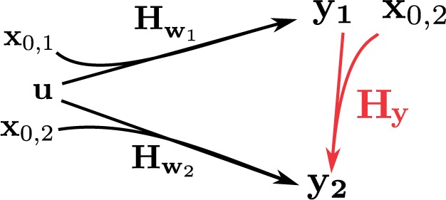
Schematic representation of the linear relationships between variables $u,x_{0,1},x_{0,2},y_1$ and $y_2$. Arrows indicate the linear relationships derived in Section 2.2

and n₁, n₂ are the lengths of vectors $x_1(t),x_2(t)$.

By lumping this chain into a single transformation matrix $H_y=H_{w_2}{H}_2{H}_1$ we obtain

$$H_y\left(\begin{array}{c}{x}_{0,2}\\ y_1\end{array}\right)=y_2,$$

and $y_1$ can be estimated from observations of $y_2$ using Tikhonov regularization with GCV, as explained in the previous section.

3 Estimation of gene expression profiles from fluorescent reporter gene data

In this section, we will show how recurring problems in the analysis of reporter gene data, the estimation of growth rate, promoter activity and protein concentration, can be mapped to the linear inversion problems formulated above. We apply the resulting methods to the analysis of fluorescent and absorbance signals measured in population-level experiments in E. coli, in conditions involving time-varying changes in growth rate and gene expression.

3.1 Fluorescent reporter gene experiments in E. coli

Changes in the environment trigger a variety of responses in bacterial cells, affecting intracellular metabolite pools within seconds and, on a longer time-scale, protein concentrations and physical parameters like cell size. The regulatory networks controlling these adaptations are complex and only partially understood.

In this article, we consider four genes playing a key role in the adaptation of E. coli to perturbations due to the sudden availability or depletion of carbon sources in the medium. These genes are fis, encoding a global regulator responsible in particular for activating ribosomal RNA transcription (Bradley et al., 2007); gyrA, coding for DNA gyrase which negatively supercoils DNA (Travers and Muskhelishvili, 2005); crp, whose product regulates the transcription of hundred of genes when activated by the secondary messenger cyclic adenosine monophosphate (cAMP) (Gosset et al., 2004) and acs, encoding an enzyme required for acetate consumption (Wolfe, 2005). We used reporter strains obtained by transforming the E. coli wild-type strain with reporter plasmids carrying a transcriptional fusion of the promoter region of the above genes with a gfp reporter gene. The reporter genes for acs and crp code for GFPmut2, a reporter with a long half-live (19 h), whereas the other reporter genes code for GFPmut3, with a short half-live of 1 h (Supplementary Section S4 for details on the plasmids and strains used in this study).

Overnight stationary-phase cultures of the reporter strains were diluted into the wells of a microplate containing minimal medium with glucose. The bacteria were observed in a microplate reader up until a few hours after glucose exhaustion (Supplementary Section S4 for details on the experimental conditions). The carbon upshift provokes a strong activation of the expression of many genes, while growth arrest following glucose exhaustion triggers the activation of so-called catabolite genes, responsible for the assimilation of secondary carbon sources, such as acetate secreted during rapid growth on glucose (Baptist et al., 2013; Enjalbert et al., 2013; Kao et al., 2005). The absorbance (600 nm) and fluorescence (485/520 nm) of the growing bacterial cultures was measured for each of the 96 wells, typically one measurement per minute per well.

The absorbance (optical density) measurements are usually assumed proportional to the volume $V(t)\in {\mathbb{R}}_{+}$ of the growing cell population. More precisely, for measurements made at time-points t_i, we have the following measurement model:

$$\tilde{V}(t_i)=\alpha V(t_i)+{\nu }_i,$$ (11)

where $\tilde{V}(t_i)$ represents the absorbance measurement at t_i, $\alpha \in {\mathbb{R}}_{+}$ an unknown proportionality coefficient, and ν_i measurement noise. We assume that the fluorescence measurements have been corrected for autofluorescence of the bacteria. Here, we simply subtracted the fluorescence time-course profile of a control strain carrying no reporter plasmid, but in other situations more sophisticated methods for background correction may need to be used, so as to avoid bias (Lichten et al., 2014; Stefan et al., 2015). The resulting fluorescence signal can be assumed proportional to the total quantity of active (mature) fluorescent protein R(t) in the growing cell population:

$$\tilde{R}(t_i)=\beta R(t_i)+\nu {\prime }_i,$$ (12)

where $\tilde{R}(t_i)$ represents the fluorescence measurement at t_i, $\beta \in {\mathbb{R}}_{+}$ an unknown proportionality coefficient, and $\nu {\prime }_i$ measurement noise.

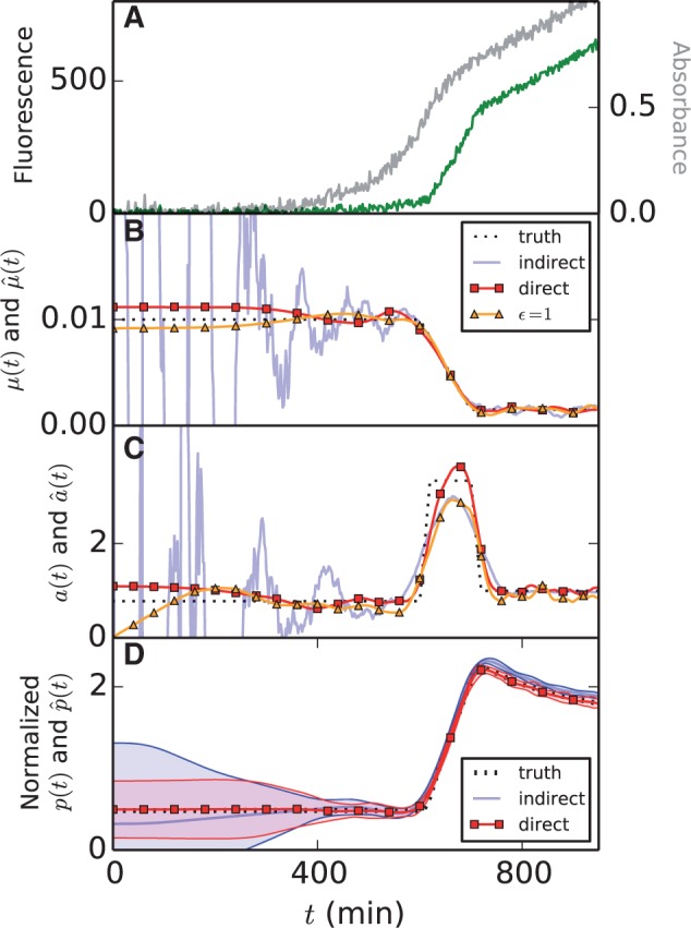
The absorbance and fluorescent measurements that will be used hereafter are shown in the top row of Figure 3. The data illustrate some of the difficulties encountered in the analysis, namely weak signals in the beginning of the experiment, when the volume of the cell population is low, and rapid changes during growth transitions.

Fig. 3.

Fluorescence and absorbance data obtained from reporter gene experiments in E. coli and estimations of growth rate, promoter activity and protein concentration from these data. The measured fluorescence and absorbance signals are shown in the top row. The estimations of growth rate, promoter activity and protein concentration are denoted by $\widehat{\mu }(t),\widehat{a}(t)$ and $\widehat{p}(t)$, respectively. The fluorescence signal, $\widehat{a}(t)$, and $\widehat{p}(t)$ have been divided by their mean as they have different orders of magnitude for genes fis, gyrA, crp and acs. For each signal, four replicates are shown, corresponding to different wells of the microplate

3.2 Estimation of growth rate

The exhaustion of glucose in the medium around 500 min is followed by growth arrest, causing a break in the absorbance curves (Fig. 3). In order to sharply distinguish the growth phases, it is important to precisely estimate the growth rate of the population, defined by

$$\mu (t)=\frac{1}{V(t)}\frac{d}{dt}V(t)=\frac{d}{dt}\log V(t).$$ (13)

It is possible to compute $\mu (t)$ from the absorbance measurements $\tilde{V}(t_i)$ of the volume V(t), by smoothing interpolation, subsequent differentiation and numerical resolution of Equation (13). However, this method is unstable when the signal-to-noise ratio is low, especially in the early stages of the experiment. Moreover, measurements of V(t) can exhibit a high noise-to-signal ratio and even be negative at times, which prohibits the use of $\log V$ as an input variable.

As an alternative approach, we formulate the problem as a linear inversion problem. We first rewrite Equation (13) as

$$\frac{d}{dt}(\alpha V)(t)=\alpha V(t)\mu (t)\simeq \tilde{V}(t)\mu (t),$$ (14)

where $\tilde{V}(t)$ is an interpolated version of the measurements $\tilde{V}(t_i)$. Replacing the volume by the experimentally measured absorbance signal has the advantage of bringing the equation into the form of Equation (1) (we use scalars to represent 1D vectors and matrices in order to simplify the notation):

$$\begin{array}{l}u(t)=\mu (t),x(t)=\alpha V(t),y(t)=\alpha V(t)\\ A(t)=0,B(t)=\tilde{V}(t),C(t)=1.\end{array}$$

That is, the growth rate is the input and the volume the output of a linear system, so that the growth rate can be estimated by linear inversion from the absorbance measurements.

The observation matrix $H_w$ for this system can be computed as explained in Supplementary Section S3.1. Solving the problem of Equations (8) and (9) by regularization, we obtain the estimates $\widehat{\mathit{\mu }}$ and ${\widehat{V}}_0$ of the growth rate and the initial volume, respectively. The growth rate estimations $\widehat{\mu }(t)$ are shown in the second row of Figure 3. As can be seen, upon glucose exhaustion the growth rate drops from its maximum value to 0. Growth arrest is abrupt in the conditions under which the data for acs and crp were acquired (Supplementary Section S4).

As our method relies on penalizing successive variations of $\mu (t)$, the question arises whether this entails a strong bias. In particular, how well estimated are the timing of the transition between the two growth phases, and the values of the growth rate during each phase? We tested the method on simulated data similar to the measurements in Figure 3, notably with equivalent sampling densities and signal-to-noise ratios. The results are presented in Supplementary Section S5. They show that our estimation method is able to recover different growth-rate profiles, with very low bias and moderate variance.

For comparison we also estimated the growth rate with the indirect method described after Equation (13). In particular, we smoothed the absorbance measurements $\tilde{V}(t_i)$ by means of smoothing splines in order to estimate the volume and its derivative, and computed an estimate of $\mu (t)$ by means of Equation (13). For simulated data shown in Figure 4A, the results in panel B show that at the beginning of the experiment, when the absorbance signal is low, the growth rate estimation is highly unstable. Additional numerical experiments, shown in Supplementary Section S5, indicate that increasing the smoothing parameter to reduce the variance of the estimates introduces a strong bias on the estimate, reflecting the well-known variance-bias trade-off. We conclude that the proposed linear inversion method performs better than this indirect approach.

Fig. 4.

Comparison of different methods for the estimation of growth rate and promoter activity from reporter gene data. We compare indirect approaches based on plugging empirically smoothed data into measurement models with the direct linear inversion methods proposed here (including a variant in which ϵ is set to 1). Additional examples can be found in Supplementary Section S5. (A) Simulated noisy absorbance data (gray) and fluorescence data (green). (B) Estimates of the growth rate $\mu (t)$ obtained with the different methods. (C) Estimates of promoter activity a(t). (D) Estimates of protein concentration p(t), using the direct method developed in this article, and an indirect method consisting in the estimation of a(t), followed by numerical solution of Equation (17). Solid lines and shaded regions represent the mean ± one standard deviation over 100 simulations. The direct methods perform better than the indirect methods in that they yield estimates with less bias and lower variance. The use of ϵ = 1 may introduce a bias

Notice that the estimation of growth rate and initial volume also leads to a denoised estimation of the population volume by Equation (5):

$$\widehat{\mathit{\alpha }V}=H_w\left(\begin{array}{cc}{\widehat{\mathit{\alpha }V}}_0& \widehat{\mathit{\mu }}\end{array}\right),$$ (15)

which will be used in the next sections for the estimation of promoter activity and protein concentration.

3.3 Estimation of promoter activity

The interest of the use of reporter genes is that, by construction, they provide information on the expression of a gene of interest. We will focus on transcriptional fusions here, where the reporter gene and the gene of interest share the same promoter region and their promoter activities can be considered identical, possibly up to a multiplicative constant (Fig. 1).

The relation between promoter activity and observed fluorescence and absorbance signals is indirect and models of gene expression are needed to interpret the primary data. Several models have been proposed in the literature (see the references in the introduction), but here we follow with some modifications the model used in de Jong et al. (2010). The expression of a fluorescent reporter gene is modeled as a three-step process involving transcription, translation and maturation of the fluorescent protein (Fig. 1). The variables of the model are $M(t),R_u(t),R(t)\in {\mathbb{R}}_{+}$, denoting the total quantity of gfp mRNA in a growing cell population and the total quantity of immature and mature Green Fluorescent Protein (GFP), respectively (in mmol). In comparison with other models, we consider total amounts of molecules and not concentrations. This has the advantage of simplifying the estimation of promoter activities, since terms due to growth dilution drop from the equations.

The rate of transcription drives the dynamics of gene expression and is defined as $k_{m}a(t)V(t)$, representing the total amount of mRNA produced per time unit in the growing cell population (mmol min⁻¹). Parameter $k_m\in {\mathbb{R}}_{+}$ represents the maximum transcription rate per unit volume, and we will call $a(t)\in {\mathbb{R}}_{+}$, which is a dimensionless quantity scaled between 0 and 1, the promoter activity. This quantity is the net effect of the different regulatory mechanisms driving the transcription of the gene, involving RNA polymerase, transcription factors and other regulators. With the constants $d_M,k_U,d_R,k_R\in {\mathbb{R}}_{+}$ (min⁻¹), characterizing the degradation, translation and maturation steps, we obtain the following ODE system:

$$\{\begin{array}{l}\frac{d}{dt}M(t)=k_{M}a(t)V(t)-d_{M}M(t),\\ \frac{d}{dt}{R}_u(t)=k_{U}M(t)-(d_R+k_R)R_u(t),\\ \frac{d}{dt}R(t)=k_R{R}_u(t)-d_{R}R(t).\end{array}$$ (16)

Notice that the transcription rate is modulated by the volume of the growing cell population, which can be replaced by its estimate from Equation (15). As a consequence, the first equation of the model writes

$$\frac{d}{dt}M(t)=k_M^{\prime }a(t)\widehat{\alpha V}(t)-d_{M}M(t),$$

where $k_M^{\prime }=k_M/\alpha$. The resulting gene expression model can be easily brought into the form of Equation (1):

$$\begin{array}{l}x(t)=\left(\begin{array}{c}M(t)\\ R_u(t)\\ R(t)\end{array}\right),A(t)=\left(\begin{array}{ccc}-d_M& 0& 0\\ k_U& -(d_R+k_R)& 0\\ 0& k_R& -d_R\end{array}\right),\\ B(t)=\left(\begin{array}{c}{k}_M^{\prime }\widehat{\alpha V}(t)\\ 0\\ 0\end{array}\right),C(t)=\left(\begin{array}{c}0\\ 0\\ \beta \end{array}\right),u(t)=a(t),\\ y(t)=\beta R(t).\end{array}$$

This allows the promoter activity a(t) as well as the initial conditions M₀, $R_{u_0}$, R₀ to be estimated from the measured fluorescence signal $\tilde{R}(t_i)$. Whereas the degradation constants d_R, d_M and the maturation constant k_R can usually be measured with high precision (de Jong et al., 2010), this is generally not the case for the other parameters. However, we prove in Supplementary Section S6 that setting $\beta ,k_U,k{\prime }_M$ to 1 still allows the time-varying profile of a(t) to be estimated, up to some unknown multiplicative coefficient (as usual in the literature).

Section 3.2 provides an efficient procedure for computing the observation matrix $H_w$ for the above system. The efficiency and accuracy of the computation of the observation matrix can be further increased when gfp mRNA is unstable and the maturation time is fast (i.e. for k_R and d_M large compared with d_R), which is the case for the reporter genes used in this study (de Jong et al., 2010). This makes it possible to lump the gene expression model of Equation (16) into a single step and thus simplify the regularized regression problem.

The linear inversion method for computing the promoter activity was applied to the reporter gene data in Figure 3, resulting in the estimates shown in the third row. We notice a sharp peak in the promoter activity of fis right after the nutrient upshift, which is consistent with previous reports (Azam et al., 1999), and the same behavior is observed for gyrA. Whereas the activity of the crp promoter shows little variation, consistent with the observation that the Crp concentration does not change much across growth phases (Kuhlman et al., 2007), upon glucose exhaustion the activity of acs shows a dramatic increase, in large part due to sudden accumulation of cAMP in the cell (Berthoumieux et al., 2013; Wolfe, 2005). These examples illustrate that the method correctly infers known fast changes in gene expression from the data, while avoiding overfitting outside the transition region.

Like in Section 3.2, we used in silico benchmarks resembling the actual data to further evaluate the ability of the method to reconstruct promoter activities, in particular the timing of the peak and its amplitude. The results in Figure 4C and Supplementary Section S5 show that the method is stable even when the signal-to-noise ratio is low, and captures the rapid variations in promoter activity with high precision. Like in Section 3.2, we remark that the method is robust, although it introduces some bias in extreme cases. However, this bias is much smaller than that obtained by an indirect method analogous to that outlined in the previous section (Fig. 4C).

The estimation of the promoter activity is interesting in its own right, as it gives insight into changes in the transcriptional activity of specific genes during growth transitions. However, it can also be the first step toward the estimation of the concentration of the regulators of a gene (Bansal et al., 2012; Finkenstädt et al., 2008) or of the concentration of the protein encoded by the gene of interest (de Jong et al., 2010). In the next section, we will develop a direct linear inversion method for addressing the latter problem.

3.4 Estimation of protein concentration

The expression of a gene of interest involves the same steps as the expression of the reporter gene, without the maturation step (Fig. 1). As explained in the previous section, in the case of transcriptional fusions the promoter activities a(t) of the two genes are the same. However, the other parameters describing mRNA and protein synthesis and degradation may be different.

In order to model the expression of the gene of interest, we introduce new variables describing the total amount of mRNA and protein for the gene of interest, denoted by N(t) and P(t) (mmol), respectively, and new kinetic constants $k_N,d_N,k_P,d_P$ (min⁻¹) representing the production and degradation rate of the mRNA and protein of interest. The protein concentration is given by $p(t)=P(t)/V(t)$. This results in the following ODE system:

$$\{\begin{array}{l}\frac{d}{dt}N(t)=k_{N}V(t)a(t)-d_{N}N(t),\\ \frac{d}{dt}P(t)=k_{P}N(t)-d_{P}P(t),\\ p(t)=P(t)/V(t).\end{array}$$ (17)

Introducing the variables $N\prime (t)=\alpha N(t)$ and $P\prime (t)=\alpha P(t)$, the system of Equation (17) becomes

$$\{\begin{array}{l}\frac{d}{dt}N\prime (t)=k_N\alpha V(t)a(t)-d_{N}N\prime (t),\\ \frac{d}{dt}P\prime (t)=k_{P}N\prime (t)-d_{P}P\prime (t)\\ p(t)=P\prime (t)/\left(\alpha V(t)\right).\end{array}$$ (18)

Like in the previous section, $\alpha V(t)$ can be replaced by the experimentally measured absorbance signal $\widehat{\alpha V}(t)$, yielding:

$$\begin{array}{l}x(t)=\left(\begin{array}{c}N\prime (t)\\ P\prime (t)\end{array}\right),A(t)=\left(\begin{array}{cc}-d_N& 0\\ k_P& -d_P\end{array}\right),u(t)=a(t),\\ B(t)=\left(\begin{array}{c}{k}_N\widehat{\alpha V}(t)\\ 0\end{array}\right),C(t)=\left(\begin{array}{c}0\\ 1/\widehat{\alpha V}(t)\end{array}\right),y(t)=p(t).\end{array}$$

For the estimation of the protein concentration p(t), the scheme outlined in Figure 2 applies, with $u(t)=a(t),y_1(t)=p(t)$, and ${\tilde{y}}_2(t)=\tilde{R}(t)$. This allows an estimate of p(t) to be obtained from the experimental measurement of R(t) as explained in Section 2.2. When the gene expression model in Equation (18) can be reduced to a single step, the observation matrix of the problem can be computed in an efficient way as explained in Supplementary Section S3.4.

The protein concentrations estimated from the E. coli reporter gene data by means of the above method are shown in the bottom row of Figure 3. The degradation constant of Fis was measured [$d_P=0.0065$ min⁻¹; de Jong et al. (2010)], whereas the other proteins were assumed to be long-lived ($d_P=0.001$ min⁻¹), like most proteins in E. coli (Larrabee et al., 1980). We observe that the Fis concentration transiently increases after the nutrient upshift, which is consistent with the role of Fis in activating the synthesis of stable RNAs necessary for growth (Dennis et al., 2004). The concentration of Crp is stable during growth on glucose and somewhat increases after glucose exhaustion, as expected from the fact that Crp activates catabolic genes needed for growth on poor carbon sources (Gosset et al., 2004). Interestingly, this accumulation cannot be simply inferred by looking at the fluorescence data, which show no increase after glucose exhaustion. It illustrates the importance of taking into account different half-lives for reporter proteins and proteins of interest.

We also tested this method on the simulated data. The results are reported in Figure 4D and show that linear inversion is more stable and introduces less bias than other approaches, notably indirect approaches based on the estimation of a(t) and numerical integration of Equation (18) using this estimate. Another advantage of the linear inversion method is that it does not need an estimate of the initial conditions, which are often unknown. In conclusion, our direct method allows rich information on gene expression to be inferred from the absorbance and fluorescence data under reasonable assumptions.

4 Software for applying linear inversion methods

As they rely on few assumptions and require virtually no hand-tuning, the linear inversion methods presented above are suitable for routine treatment of reporter gene data obtained in microplate experiments, which generate a huge quantity of measurements (typically ${10}^4-{10}^5$ data points). The linear inversion methods were implemented in the Python package WellFARE, relying on the scientific libraries NumPy and SciPy (Jones et al., 2001). In addition, the package provides utilities for parsing data files and removing outliers from the absorbance and fluorescence signals. The WellFARE package is available under an LGPL license, but has also been integrated into a web application called WellInverter, which provides a user-friendly access to the linear inversion methods through a web browser (Fig. 5). The user can upload data files by means of WellInverter, remove outliers and subtract background, and launch the procedures for computing growth rates, promoter activities, and protein concentrations (Supplementary Section S7).

Fig. 5.

Screenshot of the web application WellInverter. WellInverter allows reporter gene experiments to be analyzed online through a web-based platform. The screenshot shows background-corrected absorbance data and estimated promoter activities for three different wells (G7, G8 and G9)

5 Discussion

The inference of meaningful gene expression profiles from indirect experimental data is a key step in the analysis of dynamical models in systems biology. As reporter genes tend to become ubiquitous, it is important to develop reliable methods for the automated treatment of the large amounts of data becoming available. We have shown that the estimation of growth rate, promoter activity, and protein concentration from reporter gene data can be expressed as linear inversion problems using ODE-based measurement models and we proposed efficient procedures to compute the observation matrices solving these problems. The methods thus obtained were used to study the expression dynamics of several genes of E. coli during growth transitions, where they confirmed their ability to handle critical issues in reporter gene data analysis: low signal-to-noise ratios and rapid changes in gene expression in response to environmental perturbations. The validity of these estimation procedures was reinforced by tests on simulated data, which showed that the methods are robust and little biased.

Several methods for the analysis of reporter gene data have been proposed in the literature, all of which are implicitly or explicitly based on the same or very similar measurement models for interpreting the data. The major differences between the approaches lie in the information they extract from the data and in the way the profiles are computed from the primary data. The basic idea underlying the linear inversion methods presented here is that they are direct, in the sense that they perform regularization on the quantity to be estimated, rather than by plugging empirically smoothed versions of the data into the measurement models (de Jong et al., 2010; Ronen et al., 2002). Our results show that this improves the robustness of the estimation process. In comparison with Bansal et al. (2012), we extend the linear inversion methods to growth rates and protein concentrations, thus more fully exploiting the information contained in reporter gene data. Moreover, we improve the practical applicability of the approach in that we do not need to make assumptions that are often not realistic, such as zero initial promoter activities, constant growth rate and direct measurements of reporter concentrations. The linear inversion methods remain tractable when improving estimation through the addition of linear constraints (e.g. to ensure positive promoter activities and protein concentrations), the consideration of uncertainty on the data, or the use of different regularizations (L₁ regularization or regularization on the second derivative) (de Nicolao et al., 1997).

The methods described in this article are made available as a Python package and can also be accessed through a user-friendly web application. Other tools for the analysis of reporter gene data are WellReader (Boyer et al., 2010) and BasyLICA (Aïchaoui et al., 2012). Although the Matlab program WellReader uses the indirect approaches from de Jong et al. (2010), BasyLICA is based on the use of Kalman filters, which also directly estimate quantities of interest from the reporter gene data by a Bayesian approach. In comparison with BasyLICA, WellInverter estimates not only promoter activities but also protein concentrations from the data, and bases the inference of these quantities at a given time t not only on past data, at time-points preceding t, but on the entire dataset. In addition, WellInverter uses regularization based on GCV to avoid hand-tuning.

The generality of the techniques used in this paper suggests that they could be applied to a much wider range of problems. A necessary condition for the application of the methods is that the measured data is linearly related to the biological quantity of interest. Notice that this does not exclude time-varying parameters in Equations (16) or (17), for instance a time-varying degradation constant of the protein, due to a change in half-live after a growth transition (Hengge-Aronis, 2002). As long as the time-varying parameters are known, for example when their profile has been measured, the inversion problem remains linear. To some extent, this even allows non-linear estimation problems to be handled in our framework, as illustrated by the growth-rate estimation in Section 3.2.

The methods proposed in this article provide the most general and comprehensive treatment of the reconstruction of gene expression profiles form reporter gene data available today, based on a solid mathematical foundation and supported by user-friendly computer tools. The approach directly carry over to luminescent reporter genes and may also apply to time-series data obtained by completely different experimental technologies, like DNA microarrays, RNA-Seq or quantitative proteomics. Although we validated and illustrated the methods by means of reporter gene data from bacterial kinetics, the measurement models of Equations (16) and (17) are sufficiently general to apply to higher organisms as well.

References

- Aïchaoui L., et al. (2012) BasyLiCA: a tool for automatic processing of a bacterial live cell array. Bioinformatics, 28, 2705–2706. [DOI] [PubMed] [Google Scholar]
- Azam T.A., et al. (1999). Growth phase-dependent variation in protein composition of the Escherichia coli nucleoid. J. Bacteriol., 181, 6361–6370. [DOI] [PMC free article] [PubMed] [Google Scholar]
- Bansal L., et al. (2012) Determining transcription factor profiles from fluorescent reporter systems involving regularization of inverse problems. In Proceedings of 2012 American Control Conference (ACC 2012), Fairmont Queen Elizabeth, Montréal, Canada, pp. 2725–2730. [Google Scholar]
- Bansal M., et al. (2007) How to infer gene networks from expression profiles. Mol. Syst. Biol., 3, 78. [DOI] [PMC free article] [PubMed] [Google Scholar]
- Baptist G., et al. (2013) A genome-wide screen for identifying all regulators of a target gene. Nucleic Acids Res., 41, e164. [DOI] [PMC free article] [PubMed] [Google Scholar]
- Bertero M. (1989) Linear inverse and ill-posed problems. Adv. Electron. Electron Phys., 75, 1–120. [Google Scholar]
- Berthoumieux S., et al. (2013) Shared control of gene expression in bacteria by transcription factors and global physiology of the cell. Mol. Syst. Biol., 9, 634. [DOI] [PMC free article] [PubMed] [Google Scholar]
- Boyer F., et al. (2010) WellReader: a MATLAB program for the analysis of fluorescence and luminescence reporter gene data. Bioinformatics, 26, 1262–1263. [DOI] [PubMed] [Google Scholar]
- Bradley M., et al. (2007) Effects of Fis on Escherichia coli gene expression during different growth stages. Microbiology, 153, 2922–2940. [DOI] [PubMed] [Google Scholar]
- Chen C. (1970) Introduction to Linear System Theory. Holt, Rinehart and Winston, New York. [Google Scholar]
- Chudakov D., et al. (2010) Fluorescent proteins and their applications in imaging living cells and tissues. Physiol. Rev., 90, 1103–1163. [DOI] [PubMed] [Google Scholar]
- de Jong H., et al. (2010) Experimental and computational validation of models of fluorescent and luminescent reporter genes in bacteria. BMC Syst. Biol., 4, 55. [DOI] [PMC free article] [PubMed] [Google Scholar]
- de Nicolao G., et al. (1997) Nonparametric input estimation in physiological systems: problems, methods, and case studies. Automatica, 33, 851–870. [Google Scholar]
- de Smet R., Marchal K. (2010) Advantages and limitations of current network inference methods. Nat. Rev. Microbiol., 8, 717–729. [DOI] [PubMed] [Google Scholar]
- Dennis P., et al. (2004) Control of rRNA synthesis in Escherichia coli: a systems biology approach. Microbiol. Mol. Biol. Rev., 68, 639–668. [DOI] [PMC free article] [PubMed] [Google Scholar]
- Enjalbert B., et al. (2013) Physiological and molecular timing of the glucose to acetate transition in Escherichia Coli. Metabolites, 3, 820–837. [DOI] [PMC free article] [PubMed] [Google Scholar]
- Finkenstädt B., et al. (2008) Reconstruction of transcriptional dynamics from gene reporter data using differential equations. Bioinformatics, 24, 2901–2907. [DOI] [PMC free article] [PubMed] [Google Scholar]
- Gerosa L., et al. (2013) Dissecting specific and global transcriptional regulation of bacterial gene expression. Mol. Syst. Biol., 9, 658. [DOI] [PMC free article] [PubMed] [Google Scholar]
- Giepmans B., et al. (2006) The fluorescent toolbox for assessing protein location and function. Science, 312, 217–224. [DOI] [PubMed] [Google Scholar]
- Golub G.H., et al. (1979) Generalized cross-validation as a method for choosing a good Ridge parameter. Technometrics, 21, 215–223. [Google Scholar]
- Gosset G., et al. (2004) Transcriptome analysis of Crp-dependent catabolite control of gene expression in Escherichia coli. J. Bacteriol., 186, 3516–3524. [DOI] [PMC free article] [PubMed] [Google Scholar]
- Hansen P. (1992) Analysis of discrete ill-posed problems by means of the L-curve. SIAM Rev., 34, 561–580. [Google Scholar]
- Hengge-Aronis R. (2002) Signal transduction and regulatory mechanisms involved in control of the σS (RpoS) subunit of RNA polymerase. Microbiol. Mol. Biol. Rev., 66, 373–395. [DOI] [PMC free article] [PubMed] [Google Scholar]
- Hoerl A., Kennard R. (1970) Ridge regression: biased estimation for nonorthogonal problems. Technometrics, 12, 55–67. [Google Scholar]
- Jones E., et al. (2001) SciPy: Open Source Scientific Tools for Python. http://www.scipy.org/ (6 May 2015, date last accessed). [Google Scholar]
- Kao K., et al. (2005) A global regulatory role of gluconeogenic genes in Escherichia coli revealed by transcriptome network analysis. J. Biol. Chem., 280, 36079–36087. [DOI] [PubMed] [Google Scholar]
- Keren L., et al. (2013) Promoters maintain their relative activity levels under different growth conditions. Mol. Syst. Biol., 9, 701. [DOI] [PMC free article] [PubMed] [Google Scholar]
- Kuhlman T., et al. (2007) Combinatorial transcriptional control of the lactose operon of Escherichia coli. Proc. Natl. Acad. Sci. U.S.A., 104, 6043–6048. [DOI] [PMC free article] [PubMed] [Google Scholar]
- Larrabee K., et al. (1980) The relative rates of protein synthesis and degradation in a growing culture of Escherichia coli. J. Biol. Chem., 255, 4125–4130. [PubMed] [Google Scholar]
- Leveau J., Lindow S. (2001) Predictive and interpretive simulation of green fluorescent protein expression in reporter bacteria. J. Bacteriol., 183, 6752–6762. [DOI] [PMC free article] [PubMed] [Google Scholar]
- Lichten C., et al. (2014) Unmixing of fluorescence spectra to resolve quantitative time-series measurements of gene expression in plate readers. BMC Biotechnol., 14, 11. [DOI] [PMC free article] [PubMed] [Google Scholar]
- Porreca R., et al. (2010) Structural identification of unate-like genetic network models from time-lapse protein concentration measurements. In: Proceedings of 49th IEEE Conference on Decision and Control (CDC 2010), Atlanta, GA, USA. IEEE, pp. 2529–2534. [Google Scholar]
- Ronen M., et al. (2002) Assigning numbers to the arrows: parameterizing a gene regulation network by using accurate expression kinetics. Proc. Natl. Acad. Sci. U.S.A., 99, 10555–10560. [DOI] [PMC free article] [PubMed] [Google Scholar]
- Stefan D., et al. (2015) Inference of quantitative models of bacterial promoters from time-series reporter gene data. PLoS Comput. Biol., 11, e1004028. [DOI] [PMC free article] [PubMed] [Google Scholar]
- Travers A., Muskhelishvili G. (2005) DNA supercoiling: a global transcriptional regulator for enterobacterial growth? Nat . Rev. Microbiol., 3, 157–169. [DOI] [PubMed] [Google Scholar]
- Villaverde A., Banga J. (2014) Reverse engineering and identification in systems biology: strategies, perspectives and challenges. J. R. Soc. Interface, 11, 20130505. [DOI] [PMC free article] [PubMed] [Google Scholar]
- Wahba G. (1990) Spline Models for Observational Data. SIAM, Philadelphia, PA. [Google Scholar]
- Wang X., et al. (2008) Mathematical analysis and quantification of fluorescent proteins as transcriptional reporters. Biophys. J., 94, 2017–2026. [DOI] [PMC free article] [PubMed] [Google Scholar]
- Wolfe A.J. (2005) The acetate switch. Microbiol. Mol. Biol. Rev., 69, 12–50. [DOI] [PMC free article] [PubMed] [Google Scholar]
Associated Data
This section collects any data citations, data availability statements, or supplementary materials included in this article.