Exploring the structure and function of temporal networks with dynamic graphlets

Abstract

Motivation: With increasing availability of temporal real-world networks, how to efficiently study these data? One can model a temporal network as a single aggregate static network, or as a series of time-specific snapshots, each being an aggregate static network over the corresponding time window. Then, one can use established methods for static analysis on the resulting aggregate network(s), but losing in the process valuable temporal information either completely, or at the interface between different snapshots, respectively. Here, we develop a novel approach for studying a temporal network more explicitly, by capturing inter-snapshot relationships.

Results: We base our methodology on well-established graphlets (subgraphs), which have been proven in numerous contexts in static network research. We develop new theory to allow for graphlet-based analyses of temporal networks. Our new notion of dynamic graphlets is different from existing dynamic network approaches that are based on temporal motifs (statistically significant subgraphs). The latter have limitations: their results depend on the choice of a null network model that is required to evaluate the significance of a subgraph, and choosing a good null model is non-trivial. Our dynamic graphlets overcome the limitations of the temporal motifs. Also, when we aim to characterize the structure and function of an entire temporal network or of individual nodes, our dynamic graphlets outperform the static graphlets. Clearly, accounting for temporal information helps. We apply dynamic graphlets to temporal age-specific molecular network data to deepen our limited knowledge about human aging.

Availability and implementation: http://www.nd.edu/∼cone/DG.

Contact: tmilenko@nd.edu

Supplementary information: Supplementary data are available at Bioinformatics online.

1 Introduction

1.1 Motivation

Networks (or graphs) are powerful models of complex systems in various domains, from biological cells to societies to the Internet. Traditionally, due to limitations of data collection techniques, researchers have mostly focused on studying the static network representation of a given system (Newman, 2010). However, many real-world systems are not static but change over time (Holme and Saramäki, 2012). With new technological advancements, it has become possible to record temporal changes in network structure (or topology), corresponding to arrival or departure times of nodes or edges. Examples of temporal networks include cellular (Przytycka et al., 2010), functional brain (Valencia et al., 2008), person-to-person communication (Priebe et al., 2005), online social (Leskovec et al., 2008) or citation (Leskovec et al., 2005) networks.

The increasing availability of temporal real-world networks, while opening new opportunities, has also raised new challenges for researchers. Namely, despite a large arsenal of powerful methods that already exist for studying static networks, these methods cannot be directly applied to temporal networks. Instead, the simplest approach to deal with a temporal network is to completely discard its time dimension by aggregating all nodes and edges from the temporal data into a single static network. While this would allow to directly apply to the resulting aggregate network the existing and well-established methods for static network analysis, such an aggregate or static approach loses all important temporal information from the data. To overcome this, one could model the temporal network as a series of snapshots, each of which is a static network that aggregates the temporal data observed during the corresponding time interval. Then, with such a snapshot-based network representation, one could use a static-temporal approach to study each snapshot independently via the existing methods for static network analysis and then consider time-series of the results. However, this strategy treats each network snapshot in isolation and discards relationships between the different snapshots. Clearly, both static and static-temporal approaches overlook temporal information that is important for studying a dynamic system (Holme and Saramäki, 2012). Therefore, proper analysis of temporal networks requires development of novel strategies that can fully exploit the temporal information from the data. This is the focus of our study.

1.2 Related work

1.2.1 Static networks

One way to study the structure of a static network is to compute its global properties such as the degree distribution, diameter or clustering coefficient (Kuchaiev et al., 2011; Newman, 2010). However, although global network properties can summarize the structure of the entire network in a computationally efficient manner, they are not sensitive enough to capture detailed topological characteristics of the complex real-world networks (Pržulj, 2011). Thus, local properties have been proposed that can capture more detailed aspects of complex network structure. For example, one can study small partial subgraphs called network motifs that are statistically significantly over-represented in a network compared with some null model (Milo et al., 2002, 2004). The practical usefulness of network motifs has been questioned, since the choice of null model can significantly affect the results (Artzy-Randrup et al., 2004), and since selecting an appropriate null model is not a trivial task (Milenković et al., 2009). To address this issue, graphlets have been proposed (Pržulj et al., 2004), which are small induced subgraphs of a network that can be employed without reference to a null model (Fig. 1a), unlike network motifs. Also, unlike network motifs, graphlets must be induced subgraphs, whereas motifs are partial subgraphs, which makes graphlets more precise measures of network topology compared to motifs (Pržulj, 2011).

Fig. 1.

Illustration of the difference between static and dynamic graphlets. (a) All nine static graphlets with up to four nodes, along with their 15 ‘node symmetry groups’ (or formally, automorphism orbits) (Milenković and Pržulj, 2008; Pržulj et al., 2004). Within a given graphlet, different orbits are denoted by different node colors. For example, there is a single orbit in graphlet G₂, as all three nodes are topologically identical to each other. But there are two orbits in graphlet G₂, as the two end nodes are topologically identical to each other but not to the middle node (and vice versa). (b) All dynamic graphlets with up to three events, along with their automorphism orbits. Multiple events along the same edge are separated with commas. Node colors correspond to different orbits. (c) All four dynamic graphlets D_i whose static backbone is G₁

Graphlets have been proven in static network research. They were used as a basis for sensitive measures of network (Pržulj, 2007; Pržulj et al., 2004) or node (Milenković and Pržulj, 2008) similarities. These measures in turn have been used to develop state-of-the-art algorithms for many computational problems such as network comparison (Lugo-Martinez and Radivojac, 2014; Malod-Dognin and Pržulj, 2014; Vacic et al., 2010; Wong et al., 2014; Yaveroğlu et al., 2014), alignment (Hsieh and Sze, 2014; Kuchaiev et al., 2010; Milenković et al., 2010b; Saraph and Milenković, 2014), clustering (Hulovatyy et al., 2014a; Solava et al., 2012) or de-noising (Hulovatyy et al., 2014b), as well as for various application problems in computational biology, such as studying human aging (Faisal et al., 2014; Faisal and Milenković, 2014), cancer (Ho et al., 2010; Milenković et al., 2010a) and other diseases (Wang et al., 2014), pathogenicity (Milenković et al., 2011; Solava et al., 2012) or receptor–ligand interactions (Singh et al., 2014).

1.2.2 Temporal networks

Just as static networks, temporal networks can be studied by considering evolution of their global properties (Leskovec et al., 2005; Nicosia et al., 2012). Since this again leads to imprecise insights into network changes with time, recent focus has shifted onto local-level dynamic network analysis via notion of ‘temporal motifs’. In the simplest case of the static-temporal approach, static motifs are counted in each snapshot and then their counts are compared across the snapshots (Braha and Bar-Yam, 2009). To overcome this approach’s limitation of ignoring any motif relationships between different snapshots, the notion of static network motifs has been extended into several notions of temporal motifs (Bajardi et al., 2011; Chechik et al., 2008; Jurgens and Lu, 2012; Kovanen et al., 2011, 2013; Zhao et al., 2010). However, the temporal motif approaches suffer from the following drawbacks. (1) They only deal with motif structures of limited size or topological complexity (e.g. linear paths) (Bajardi et al., 2011; Jurgens and Lu, 2012; Zhao et al., 2010), which limits their practical usefulness to capture complex network structure in detail. (2) They pose additional constraints, such as limiting the number of events (temporal edges) a node can participate in at a given time point (Kovanen et al., 2011, 2013). (3) They allow for obtaining the motif-based topological ‘signature’ of the entire network only but not of each individual node (Bajardi et al., 2011; Braha and Bar-Yam, 2009; Chechik et al., 2008; Jurgens and Lu, 2012; Kovanen et al., 2011, 2013; Zhao et al., 2010), whereas the latter is useful when aiming to link the network topological position of a node to its function via, e.g. network alignment or clustering. (4) Importantly, like static motifs, all temporal motif approaches rely on a null model, which again questions their practical usefulness (Artzy-Randrup et al., 2004; Milenković et al., 2008, 2009), especially since choosing an adequate null model is even harder in the dynamic than static setting.

Analogous to extending the notion of network motifs from the static to dynamic setting, recently, we used graphlets as a basis of a static-temporal approach to study human aging from biological networks (Faisal and Milenković, 2014). We counted static graphlets within each snapshot (corresponding to a given human age), and then we studied the time-series of the results to gain insights into network structural changes with age (Faisal and Milenković, 2014). In this initial study, we only used the static graphlets within a static-temporal approach that ignored important relationships between different snapshots, in order to demonstrate that accounting for at least some temporal information in the static-temporal fashion can improve results compared with using the traditional static (aggregate) approach. Further important temporal inter-snapshot information remains to be explored via a novel truly temporal approach. We aim to develop such an approach, as follows.

1.3 Our contribution

To overcome the issues of the existing methods for temporal network analysis, we take the well-established static graphlets to the next level to develop new theory of dynamic graphlets that allow for efficient temporal analysis. Unlike the existing temporal motif approaches, our dynamic graphlets allow for all of the following. (1) They can study topological and temporal structures of arbitrary complexity, as permitted by available computational resources. (2) There are no limitations on, e.g. the number of events that a node can participate in. (3) They can capture the topological signature of the entire network and of each individual node. (4) They allow for studying temporal networks without relying on a null model. Also, unlike the existing static-temporal graphlet approach, dynamic graphlets explicitly account for inter-snapshot relationships.

Of the existing methods, the closest to our study are temporal motifs as defined in Kovanen et al.. (2011), static graphlets (Milenković and Pržulj, 2008; Pržulj et al., 2004) and static-temporal graphlets (Faisal and Milenković, 2014). Since temporal motifs depend on a null model and have other limitations, they cannot be directly and fairly compared with our dynamic graphlets. Static and static-temporal graphlets are directly comparable with our dynamic graphlets. By comparing the different graphlet approaches, we can fairly evaluate the effect on result accuracy of the amount of temporal information that each graphlet approach can consider.

In the rest of the article, we formally define our novel notion of dynamic graphlets (Section 2). We thoroughly evaluate their ability to characterize the structure and function of an entire temporal network as well as of individual nodes. Namely, on both synthetic and real-world temporal network data, we measure how well our approach can group (i.e. cluster) temporal networks (or nodes) of similar structure and function and separate dissimilar networks (or nodes). We find that our dynamic graphlet approach outperforms both static and static-temporal graphlet approaches in all of these tasks (Section 3). This confirms our hypothesis that accounting for more temporal information helps. We demonstrate one possible application of dynamic graphlets: to study age-specific structural and functional changes in the cell from temporal aging-related molecular network data of human (Section 3.4).

2 Methods

We introduce dynamic graphlets in Section 2.1, give an algorithm for their counting in Section 2.2 and describe our evaluation in Section 2.3.

2.1 Dynamic graphlets

Let G(V, E) be a temporal network, where V is the set of nodes and E is the set of events (temporal edges) that are associated with a start time and duration (Holme and Saramäki, 2012). An event can be represented as a 4-tuple $(u,v,t_{\text{start}},\sigma )$, where u and v are its endpoint nodes, t_start is its starting time and σ is its duration. Thus, each event is linked to a unique edge in the aggregate static network, whereas each static edge may be linked to multiple events with different starting times. Note that here we consider undirected events, but most ideas can be extended to directed events as well.

Given a temporal network (as defined above), our goal is to extend the notion of static graphlets in order to capture how the network neighborhood of a node changes over time. For example, since multiple events can occur over the same edge, the same static graphlet G₁ (Fig. 1a) can correspond to multiple dynamic graphlets (defined below), such as D₄ and D₆ (Fig. 1b), depending on the order of events in the temporal network. For this reason, we aim to develop methodology that allows for distinguishing between such different temporal network structures.

To formalize this desired intuition of dynamic graphlets, we first introduce the notion of a time-respecting path, whose goal is to connect two nodes so that for any two consecutive events in the path, the later event starts no later than $\Delta t$ time after the earlier event ends (i.e. so that the two events are $\Delta t$-adjacent). Formally, we say that two nodes s and d are connected by a $\Delta t$-time-respecting path if there is a sequence of events $(v_0,u_0,t_0,{\sigma }_0),(v_1,u_1,t_1,{\sigma }_1)$, $\dots ,(v_k,u_k,t_k,{\sigma }_k)$, such that $v_0=s$, u_k = d, $\forall i\in [0,k-1]$ $u_i=v_{i+1}$ and $t_{i+1}\in [t_i+{\sigma }_i,t_i+{\sigma }_i+\Delta t]$. The above $\Delta t$ constraint allows a user to control how much time (at most) can pass between two events so that they are considered to be consecutive (i.e. $\Delta t$-adjacent).

Given the above definitions, a temporal network is called $\Delta t$-connected if for any (unordered) pair of nodes there exists a $\Delta t$-time-respecting path between the two nodes. Also, we define a $G\prime (V\prime ,E\prime )$ to be a temporal subgraph of G with $V\prime \subseteq V$ and $E\prime \subseteq E$, where $E\prime$ is restricted to nodes in $V\prime$. Then, a dynamic graphlet is an equivalence class of isomorphic $\Delta t$-connected temporal subgraphs; equivalence is taken with respect to the relative temporal order of events, without considering the events’ actual start times. Hence, two $\Delta t$-connected temporal subgraphs will correspond to the same dynamic graphlet if they are topologically equivalent and their corresponding events occur in the same order. Figure 1b illustrates all dynamic graphlets with up to three events, but we evaluate larger graphlets as well.

Note that if for a given dynamic graphlet with n nodes and k events we discard the order of the events and remove duplicate events over the same edge, we get a static graphlet with n nodes and $k\prime \le k$ edges (e.g. G₁ from D₆), which we call the backbone of the dynamic graphlet. Each dynamic graphlet has a single backbone, while one backbone can correspond to different dynamic graphlets (Fig. 1c and Supplementary Table S1).

The above definitions allow us to describe all dynamic graphlets of a given size in the entire network, in order to obtain topological signature of the network. There already exists a popular notion of topological signature of an individual node in a static network, called the graphlet degree vector (GDV) of the node, which describes the number of each of the static graphlets that the node ‘touches’ at a specific ‘node symmetry group’ (or automorphism orbit) (Fig. 1a) (Milenković and Pržulj, 2008). Here, we aim to describe the node’s dynamic GDV equivalent. In this case, automorphism orbits of a dynamic graphlet will be determined based on both topological (as in static case) and temporal (unlike in static case) positions of a node within the dynamic graphlet. Thus, a dynamic graphlet with n > 2 nodes will have n different orbits (Fig. 1b), whereas the number of orbits in a static graphlet of size n is typically less than n (Fig. 1a); only for a dynamic graphlet with n = 2 (e.g. D₃), there will be only one orbit, since events are undirected and thus the two end nodes in such a graphlet are topologically equivalent.

Next, we aim to compute D(n, k), the number of dynamic graphlet types with n nodes and k events. Since at least n – 1 edges are needed to connect n nodes, it follows that $D(n,k)=0$ for $k<n-1$. Further, since our events are undirected, if follows that $D(2,k)=1$, for any k. To compute D(n, k) when $n\ge 3$ and $k\ge n-1$, notice that each dynamic graphlet with k events can be formed from a dynamic graphlet with k – 1 events and either n – 1 or n nodes, by adding a new event between some two existing nodes or between an existing node and a new node, respectively (Fig. 2). From these observations, we get the following recursive formulas for D(n, k): $D(3,k)=3D(3,k-1)+D(2,k-1),n=3$ and $D(n,k)=(2n-3)D(n,k-1)+2D(n-1,k-1),n>3$, plus the corresponding closed-form solution (Supplementary Section S1 and Table S2):

$$D(n,k)={\displaystyle \sum _{i=0}^{n-2}\frac{{(-1)}^{n+i}\left(\begin{array}{c}n-2\\ i\end{array}\right){(2i+1)}^{k-1}}{2(n-2)!}},n\ge 3.$$

Since now we can compute D(n, k), we next consider the task of enumerating and generating each of these dynamic graphlet types (in Section 2.2, we discuss the process of counting each of the generated graphlets in a given network). We build upon the fact that each dynamic graphlet with k events has a unique $(k-1)$-‘prefix’ (see above). Thus, we start with a single event (dynamic graphlet D₀ with n = 2 and k = 1) as the current graphlet and then recursively extend the current graphlet until the desired size is reached. Supplementary Algorithm S1 illustrates our enumeration procedure.

Fig. 2.

Illustration of how we extend a dynamic graphlet with an additional more recent event, on the example of D₉. There are seven possible extensions of D₉ (which contains four nodes and three events) with the most recent event 4 (shown in bold) into a dynamic graphlet with four events. Five of the extensions keep the same number of nodes but increment the number of events, while the remaining two extensions increment both the number of nodes and events. Note that in order to extend D₉ with event 4, at least one of the nodes involved in event 3 has to participate in event 4 as well

2.2 Counting dynamic graphlets in a network

As now we know the number of dynamic graphlet types of a given size and how to enumerate and generate each one of them, how to actually count each of the dynamic graphlets in a given network? Here, we discuss key ideas behind our counting procedure; for a detailed description and the corresponding algorithms, see Supplementary Section S2.

We perform dynamic graphlet counting in the same way as we generate the graphlet types. That is, for each event in a temporal network, we use this event as the current dynamic graphlet (of type D₀) and then search for larger graphlets that are grown recursively from the current one (Fig. 3). Supplementary Algorithms S2–S4 describe this procedure. Its running time depends on the structure of the given temporal network. In general, since the algorithm explicitly goes through every dynamic graphlet that it counts, the running time is proportional to the number of dynamic graphlets. For a network with D $\Delta t$-adjacent event pairs, counting all dynamic graphlets with up to k events takes $\mathcal{O}\left(\left|E\right|+\left|E\right|{\left(\frac{D}{\left|E\right|}\right)}^{k-1}\right)$. As with static graphlets, the running time of exhaustive dynamic graphlet counting is exponential in graphlet size (but is still practical, as we will show). Yet, as elegant non-exhaustive approaches were proposed for faster static graphlet counting (Hočevar and Demšar, 2014; Marcus and Shavitt, 2012; Rahman et al., 2014), similar techniques can also be sought for dynamic graphlet counting.

Fig. 3.

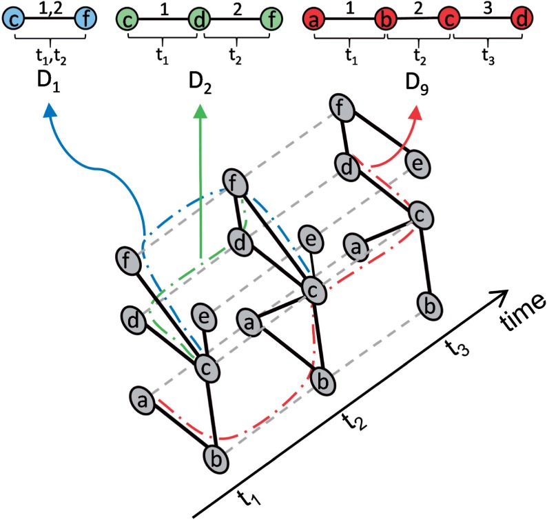
Illustration of our dynamic graphlet counting procedure. The temporal network is a sequence of three snapshots. Dashed lines denote instances of the same node in different snapshots. Colored lines denote the path of how the temporal network is explored in order to count the given dynamic graphlet. Regular dynamic graphlet counting will detect all three of the dynamic graphlets D₁ (involving nodes c and f), D₂ (involving nodes c, d and f), and D₉ (involving nodes a, b, c and d). Constrained dynamic graphlet counting (Supplementary Section S2) will detect only the first two dynamic graphlets, but not D₉. This is because nodes c and d are interacting in both the second and third snapshots. That is, according to constrained counting, the event between c and d at time t₃, which is necessary for identifying a graphlet D₉ in the network, is considered to be redundant to the event between c and d at time t₂. As such, the event between c and d at time t₃ is ignored by constrained counting and thus no D₉ can be detected

In a network having dense neighborhoods or many events over the same nodes, a given dynamic graphlet type will likely be detected more times than in a network having sparse neighborhoods and few events between the same nodes. Thus, dynamic graphlet counting in the former network type will be computationally expensive, due to having to consider a large number of occurrences of a given graphlet type. Moreover, the occurrences of a given graphlet type will likely be just artifacts of the consecutive snapshots ‘sharing’ the same (dense) network structure. Thus, we propose a modification to the counting process that is expected to reduce the count for a given dynamic graphlet type, as illustrated in Figure 3 and described in Supplementary Section S2. This modification, which we call constrained dynamic graphlet counting, is consequently expected to reduce computational complexity of the counting process compared to the regular dynamic graphlet counting procedure described above (which we will demonstrate in Section 3). Importantly, this change from regular to constrained dynamic graphlet counting affects only the count of how many times a given dynamic graphlet type appears in the network of interest; it does not affect what graphlet types will be searched for and counted in the network.

2.3 Experimental setup

2.3.1 Graphlet methods under consideration and network construction

We compare static, static-temporal, dynamic and constrained dynamic graphlets. To count static graphlets in a temporal network, we aggregate the temporal data into a single static network, by keeping the node set the same, and by adding an edge between two nodes in the static network if there are at least w events between these nodes in the temporal network. For other methods, we use a snapshot-based network representation: we split the whole time interval of the temporal network into time windows of size t_w, and for each window, we construct a static snapshot by aggregating the temporal data during this window with the parameter w, as above. We tested multiple values of w and t_w (Supplementary Section S3). Since we observed no qualitative differences in results of the different choices, we report results for w = 1 and t_w = 2, unless noted otherwise. Note that in all studied networks all events are instantaneous (i.e. ${\sigma }_i=0$ for each event e_i). Also, for static and static-temporal graphlets, we vary the number of graphlet nodes n, and for dynamic and constrained dynamic graphlets, we vary both the number of graphlet nodes n and the number of graphlet events k. Here, we report results for multiple parameter choices.

2.3.2 Network classification

An approach that captures network structure (and function) well should be able to group together similar networks (i.e. networks from the same class) and separate dissimilar networks (i.e. networks from different classes) (Yaveroğlu et al., 2014). To evaluate our (constrained) dynamic graphlets against static and static-temporal graphlets in this context, we generate a set of synthetic (random graph) temporal networks of nine different classes corresponding to nine different versions of an established network evolution model (see below) (Leskovec et al., 2008). We use synthetic temporal network data because obtaining real-world temporal network data for multiple different classes and with multiple examples per class is hard. And even if a wealth of temporal network data were available, we typically have no prior knowledge of which real-networks are (dis)similar, i.e. which networks belong to which functional class.

The network evolution model that we use was designed to simulate evolution of real-world social networks. The model is parameterized by the node arrival function that corresponds to the number of nodes in the network at a given time, a parameter that controls the lifetime of a node, and parameters that control how active the nodes are in adding new edges. By choosing different options for the model parameters, we generate networks with nine different evolution processes (Supplementary Section S3).

To test the robustness of the graphlet methods to the network size, in each of the nine network classes, we test three network sizes: 1000, 2000 and 3000 nodes. For each network size and class, we generate 25 random graph instances. We report results for the largest network size of 3000 nodes. Results for the other network sizes were qualitatively similar.

Given the resulting aggregate or snapshot-based network representations, we then compute static, static-temporal or (constrained) dynamic graphlet counts in each network and reduce the dimensionality of the networks’ graphlet vectors with principle component analysis (PCA). We consider as few PCA components as needed to account for at least 90% of variation. Here, this leads us to considering the first two PCA components. Then, we use Euclidean distance in this PCA space as a network distance measure and evaluate whether networks from the same class are closer in the graphlet-based PCA space than networks from different classes, as described below.

In addition to studying the nine versions of the above network model that was originally proposed in the domain of social networks, we perform the same analysis on four different versions of two well-established network models from the computational biology domain: geometric gene duplication model with probability cutoff (Pržulj et al., 2010) and scale-free gene duplication model (Vazquez et al., 2001). Both models start with a small initial seed network and then grow it by adding new nodes while relying on principles of gene duplication and mutation. The models were shown to mimic well evolution of protein–protein interaction networks (Pržulj et al., 2010). For more details, see Supplementary Section S3.

2.3.3 Node classification

We also evaluate whether the graphlet methods can group together similar nodes (rather than entire networks). We measure the ability of the methods to distinguish between functional node labels (i.e. classes) based on the nodes’ graphlet-based topological signatures. As a proof of concept, we do this on a publicly available Enron dataset (Priebe et al., 2005), which is both temporal and contains node labels. Unfortunately, availability of additional experimentally inferred temporal and labeled network data is limited. (In Section 3.4, we use a computationally inferred network from the computational biology domain to study human aging.) The Enron network is based on email communications of 184 users from 2000 to 2002, with seven user roles in the company as node labels: CEO, president, vice president, director, managing director, manager and employee.

For an aggregate or snapshot-based network (Supplementary Section S3), we compute static, static-temporal or (constrained) dynamic graphlet counts of each node in the network and reduce the dimensionality of the given node’s graphlet vector with PCA. Here, we need to keep the first three PCA components to account for at least 90% of variation. We use Euclidean distance as a node distance measure, and evaluate whether same-label nodes are closer in the PCA space than nodes with different labels, as follows.

2.3.4 Evaluation strategy

Given a set of objects (networks or nodes), graphlet-based PCA distances between the objects, and the objects’ ground truth classification (with respect to nine/four network classes or seven node labels), we evaluate a graphlet approach by measuring if it correctly places close (far) in the PCA space those objects whose classes match (do not match). First, we sort all object pairs in terms of their increasing distance, and consider k closest pairs. Then, we compute the accuracy in terms of precision, the fraction of class-matching pairs out of the considered pairs, and recall, the fraction of considered class-matching pairs out of all class-matching pairs (Supplementary Section S3). We find the value of k where precision and recall are equal, and we refer to this precision and recall value as the break-even point. Since lower precision means higher recall, and vice versa, we combine the two measures into F-score and report the maximum F-score over all values of k. To summarize these results over the whole [0–100%] range of k, we measure average method accuracy by computing the area under the precision-recall curve (AUPR). Also, we compute the area under the receiver operator characteristic curve (AUROC) (Supplementary Section S3). AUPRs are more credible than AUROCs when there exists imbalance between the size of the set of class-matching object pairs and non-matching pairs. With the expectation that PCA distances between class-matching pairs would be statistically significantly lower than distances of non-matching pairs, we compare two sets of distances via Wilcoxon rank-sum test (Supplementary Section S3) (Hulovatyy et al., 2014a). For each of these evaluation tests, we evaluate all graphlet methods against a random approach (Supplementary Section S3).

3 Results and discussion

We evaluate our novel (constrained) dynamic graphlet approach against the existing static and static-temporal graphlet approaches in the context of two evaluation tasks: network classification (Section 3.1) and node classification (Section 3.2). Also, we discuss the effect of different method parameters on the results (Section 3.3). We present a real-life computational biology application of dynamic graphlets in the context of studying human aging (Section 3.4).

3.1 Network classification

First, we test how well the different methods distinguish between nine classes of synthetic temporal networks based on the networks’ graphlet counts; here, the networks come from a well-established network model that was originally proposed in the social network domain. The different evaluation criteria give consistent results: while according to Wilcoxon rank-sum test, all methods have intra-class distances significantly lower than inter-class distances and thus show non-random behavior (P-values < ${10}^{-100}$), (constrained) dynamic graphlets are superior in terms of both accuracy and computational complexity, followed by static-temporal and static graphlets, respectively (Fig. 4 and Supplementary Table S3). Regular dynamic graphlets perform better than constrained dynamic graphlets in terms of accuracy; the two are comparable in terms of computational complexity (Supplementary Tables S3 and S4).

Fig. 4.

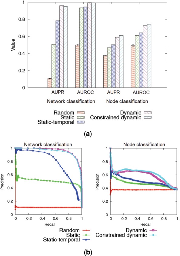
Comparison of the graphlet approaches in the context of network and node classification, in terms of (a) AUPR and AUROC values and (b) precision-recall curves. For each method, the highest-scoring graphlet size is chosen. For other parameter choices, see Supplementary Tables S3 and S5

Second, we perform the same analysis on four different classes of synthetic temporal networks that come from the computational biology domain. The results are qualitatively similar to those from Figure 4: (constrained) dynamic graphlets outperform both static and static-temporal graphlets (Supplementary Fig. S1).

3.2 Node classification

Also, we test how well the different methods distinguish between seven different classes of nodes in a real-world network based on the nodes’ graphlet counts. The different evaluation criteria give consistent results: while according to Wilcoxon rank-sum test, all methods have intra-class distances significantly lower than inter-class distances and thus show non-random behavior (P-values < ${10}^{-100}$), just as with network classification, (constrained) dynamic graphlets are again superior both in terms of accuracy and computational complexity, followed by static-temporal graphlets, followed by static graphlets (Fig. 4 and Supplementary Table S5).

Constrained dynamic graphlet counting takes significantly less time than regular dynamic graphlet counting (Supplementary Table S5), which justifies our motivation behind constrained counting. This speedup allows us to consider larger graphlet sizes (e.g. six or seven nodes) that are not attainable when using regular dynamic graphlet counting due to computational constraints. Nonetheless, constrained dynamic graphlet counting outperforms regular dynamic graphlet counting even when controlling for graphlet size (Supplementary Section S4 and Table S5).

Importantly, the four graphlet methods differ not only quantitatively (as shown above) but also qualitatively: static, static-temporal and (constrained) dynamic graphlets identify different nodes as topologically similar (Supplementary Fig. S2).

3.3 Effect of graphlet size on results

We test the effect on results of graphlet size in terms of the number of nodes as well as events (Supplementary Section S4). For network classification, increasing the values of these parameters does not always improve accuracy, while it (drastically) increases the running time of graphlet counting (Supplementary Tables S3 and S4). Thus, using smaller graphlets should suffice to achieve satisfactory accuracy at a reasonable computational complexity. On the other hand, for node classification, using larger graphlets generally improves the performance. Nonetheless, there is an effect of diminishing returns with increase of graphlet size (Supplementary Table S5). This again implies that using smaller graphlets might suffice.

The decrease of performance with increase of graphlet size in the task of network classification (but not node classification) is not alarming. Similar behavior has already been observed in static network research (Hulovatyy et al., 2014b; Yaveroğlu et al., 2014). A possible explanation for such behavior is discussed in Supplementary Section S4. Further theoretical and empirical analyses of this behavior are subject of future work.

3.4 Application to aging

3.4.1 Motivation

As susceptibility to diseases increases with age, studying human aging is important. However, doing so experimentally is hard due to long lifespan and ethical constraints. Network research can be used to deepen current limited knowledge about human aging that has been obtained mainly via other computational methods, e.g. analyses of gene expression or sequence data (Kriete et al., 2011). Here, we aim to complement existing static (Faisal et al., 2014; Ferrarini et al., 2005) or static-temporal (Faisal and Milenković, 2014) network efforts to study human aging with our new temporal approach—(constrained) dynamic graphlets.

We already used a static graphlet-based node centrality measure (Milenković et al., 2011), along with six other centrality measures, to study human aging (Section 1.2) (Faisal and Milenković, 2014). Because it is hard to experimentally obtain large-scale temporal molecular network data due to limitations of biotechnologies for data collection, we integrated the current static protein–protein interaction network of human (Peri et al., 2004) with aging-related gene expression data (Berchtold et al., 2008) to computationally infer temporal age-specific network data. Then, we predicted as aging-related those genes whose network centralities significantly changed with age. In that study, we computed centrality of each node in each snapshot and analyzed the time-series of the results. Hence, that was a static-temporal approach. The study resulted in the set of 537 aging-related gene candidates, which we called DyNetAge, and which we validated in a number of ways.

Here, we use the same temporal age-specific network data and apply our dynamic graphlets to this dataset, to see whether we can improve the prediction quality (i.e. gain additional aging-related predictions) compared with the static-temporal DyNetAge approach. Also, since the latter is quite different than our graphlet approaches from this study (as it is based on the notion of changing node centralities and on multiple measures of network topology), we also compare our dynamic graphlets to the static and static-temporal graphlet approaches from the previous sections. This allows for a fair evaluation of the effect on prediction accuracy of the amount of temporal information that each graphlet approach can consider.

3.4.2 Evaluation on known ‘ground truth’ aging-related data

Given the temporal network and two mutually exclusive node labels (i.e. classes), corresponding to ‘aging-related gene’ if the given node is present in DyNetAge or ‘non-aging-related gene’ if the given node is absent from DyNetAge, we perform the same node classification analysis as in Section 3.2: we ask whether aging-related genes are closer to each other than to non-aging-related genes in the graphlet-based PCA space (here, we need to consider the first two PCA components to account for at least 90% of variation; Section 2.3). We find that the results are consistent with those from Section 3.2: (constrained) dynamic graphlets are again superior compared with static and static-temporal graphlets (Supplementary Fig. S3). Moreover, similar results hold even when we use non-network-based ‘ground truth’ aging-related data instead of DyNetAge (Supplementary Figs S4 and S5).

The above analysis mimics precisely our node classification analysis from Section 3.2. Next, we perform a modified analysis: we do not consider the entire k range (Section 2.3) but instead focus only on high-scoring node pairs, i.e. on a low k threshold. We do this because we are interested in making as accurate predictions as possible (corresponding to higher precision) at the expense of reducing the number of predictions (corresponding to lower recall). Since precision drastically decreases as we increase k while recall barely increases (Supplementary Fig. S3), we study only the highest-scoring node pairs. For illustration purposes, we choose two such values of k: 0.00005 and 0.0001%. Since we are dealing with millions of node pairs, even such low k values result in sufficiently many (hundreds of) high-scoring node pairs. When we compare precision of the graphlet methods at each of the two values of k, our dynamic graphlets are again comparable or superior to static and static-temporal graphlets (left side of Table 1). All methods have the same (low) recall of 0.001, as expected for such small values of k. Similar results hold when we use non-network-based ‘ground truth’ aging-related data (Supplementary Table S6).

Table 1.

Precision of the different methods in the context of aging at the two k values when considering all node pairs (left) and ignoring all node pairs in which both genes are non-aging-related (right)

	Considering all node pairs		Ignoring non-aging-related node pairs
	k1	k2	k1	k2
Static	0.981	0.981	0.492	0.489
Static-temporal	0.992	0.992	0.915	0.788
Dynamic	0.998	0.998	0.983	0.784
Constrained dynamic	0.993	0.993	0.684	0.681
Random	0.850	0.851	0.041	0.035

For each method, the highest-scoring graphlet size is chosen. In a column, the value in bold is the best result over all methods.

Finally, we perform an additional analysis to evaluate the different graphlet approaches in the context of aging. Since in the following section we aim to predict novel aging-related knowledge, and since there are significantly many more non-aging-related than aging-related genes in the network data, we perform the same evaluation as above (considering the same two k values) while discarding all of the highest scoring node pairs in which both genes are non-aging-related. We do this because node pairs in which both genes are non-aging-related would mistakenly lead to high precision (this is exactly why the random approach has a high precision in the left side of Table 1). Again, we find that dynamic graphlets are overall superior to static and static-temporal graphlets (right side of Table 1). Note that the lower precision values in the previous analysis (left side of Table 1) compared with this analysis (right side of Table 1) are expected. This is because the number of false positives (gene pairs involving an aging-related gene and a non-aging-related gene) stays the same, while the number of true positives decreases (since we have removed some of the true positive gene pairs, i.e. those pairs involving two non-aging-related genes).

3.4.3 Evaluation of novel aging-related predictions

The above analysis suggests that because dynamic graphlets do not achieve precision of 1 (Table 1), they rank as high-scoring a node pair in which one gene is aging-related while the other one is not. Given this scenario, we hypothesize that the non-aging-related gene in such a pair is actually aging-related (i.e. that it was missed by the DyNetAge study) and we predict it as such. We generalize this prediction strategy to all graphlet approaches. This way, static, static-temporal, dynamic and constrained dynamic graphlets produce 84, 16, 16 and 80 novel aging-related predictions at the first k threshold and 86, 43, 47 and 81 novel predictions at the second k threshold, respectively (Supplementary Fig. S6 and Table S7).

Next, we aim to validate each approach’s predictions by measuring their gene, functional [i.e. Gene Ontology (GO)] (Ashburner et al., 2000), and disease (Du et al., 2009) overlaps with independent known ‘ground truth’ aging-related data, as described in (Faisal and Milenković, 2014). The more statistically significant and larger the overlap, the better the given approach. Here, we find that dynamic or constrained dynamic graphlets are superior to static and static-temporal graphlets in 67% of all tests, and they are comparable in the remaining 33% of all tests (Table 2). Thus, (constrained) dynamic graphlets not only improve the prediction quality of the DyNetAge approach and uncover the known aging-related knowledge more precisely than static or static-temporal graphlets, but also, more of their novel knowledge can be validated.

Table 2.

Overlaps (given as percentages of the smaller of the compared data sets), along with P-values of the overlaps (shown in parentheses), of (1) genes, (2) enriched functions and (3) enriched diseases, between each graphlet approach’s novel predictions and the three independent ‘ground truth’ aging-related datasets (BrainExpression2004Age, BrainExpression2008Age and SequenceAge), for the two k values

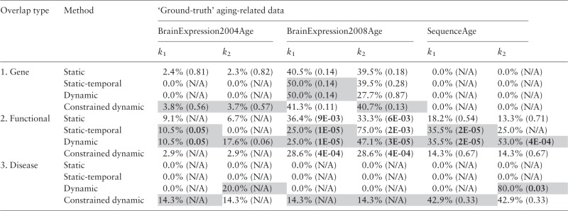The first two ‘ground truth’ datasets have been derived via gene expression analyses, whereas the latter has been derived via genomic sequence analyses; see Faisal and Milenković (2014) for details. ‘N/A’ is shown when there are fewer than two objects (genes, functions or diseases) in the overlap. Statistically significant P-values (at 0.05 threshold) are shown in bold. Note that low P-values are extremely encouraging, since we are aiming to validate novel aging-related knowledge. For the same reason, it is not necessarily discouraging when a result is not statistically significant (Faisal and Milenković, 2014). Also, note that a larger relative (percent) overlap between two sets does not necessarily mean a lower P-value, as the P-value also depends on the size of the two sets of interest; see the description of the hypergeometric test in e.g. Faisal and Milenković (2014). There are $3\times 3\times 2=18$ combinations of overlap type, ‘ground truth’ data, and value of k. For each combination, the value in gray is the best result over the four graphlet methods. By ‘best result’, we mean the lowest P-value, if at least one of the four P-values is significant; otherwise, we mean the largest overlap, unless the overlap is 0. In $12/18=67\%,6/18=33\%$, and $0/18=0\%$ of the combinations, (constrained) dynamic graphlets are superior, comparable or inferior, respectively, to static and static-temporal graphlets.

When we qualitatively zoom into the results from Table 2, we find evidence that the novel knowledge predicted by (constrained) dynamic graphlets is indeed aging-related. First, functional overlap is significant (P-values < 0.05) between dynamic graphlets and each ‘ground truth’ dataset, for each k value; only in one case, P-value is only marginally significant (0.06). Some significant functional overlaps also exist for static-temporal graphlets. For the second k value, only dynamic graphlets significantly overlap (P-value of $4\times {10}^{-4}$) with SequenceAge (de Magalhães et al., 2009), the most trusted source of ‘ground-truth’ aging-related knowledge in human obtained mainly via genomic sequence analyses. Second, for both k values, only predictions resulting from (constrained) dynamic graphlets are enriched in some diseases that the ‘ground truth’ data are also enriched in; this does not hold for static or static-temporal graphlets. Dynamic graphlets’ disease overlap with SequenceAge is significant (P-value of 0.03) for the second k value.

Zooming further into the two overlaps of DyNetAge and SequenceAge at the second value of k, while nine GO terms overlap between dynamic graphlets’ predictions and SequenceAge, eight additional GO terms are enriched in predictions of dynamic graphlets but not in those from SequenceAge (Supplementary Table S8). Similarly, while four diseases (Parkinson disease, oral cancer, chronic obstructive airway disease and embryoma) overlap between the two datasets, bipolar disorder is also enriched in dynamic graphlets’ predictions but not in SequenceAge. However, we find literature evidence that many of these GO terms and diseases that are enriched in dynamic graphlets’ predictions but not in SequenceAge are actually linked to aging. One such GO term is response to zinc ion, and we find that carnosine, which serves as a metal ion (e.g. zinc) chelator, possesses anti-aging functions [PubMed ID (PMID): 25158972]. Another such GO term is rRNA processing, and we find that human N-acetyltransferase 10 is both a promising target for therapies against premature aging and a catalyzer involved in rRNA processing (PMID: 25411247). Additional such GO terms are xenobiotic metabolic process, cellular metabolic process, cellular protein metabolic process, and we find the following. First, when analyzing gene expression profiles associated with the early steps of age-related cell transformation, bioinformatics analyses highlighted metabolic pathways, the top scoring one being the metabolism of xenobiotics by cytochrome P450 (PMID: 24929818). Second, a link has already been established between metabolism and many aging-related diseases, including Alzheimer’s disease, stroke, diabetes (PMID: 25538685). The disease enriched in dynamic graphlets’ predictions but not in SequenceAge is bipolar disorder, and we find the following. First, mood disorders, such as bipolar one, are associated with accelerated aging (Simon et al., 2006). Second, protein S100B is both elevated in mood disorders and linked to aging, with higher levels in elderly depressed subjects (PMID: 23701298). Third, bipolar disorder causes mitochondrial dysfunction (Kato and Kato, 2000), and the latter in turn is a cause of aging (PMID: 18226094). These results further validate novel aging-related predictions of dynamic graphlets. Importantly, dynamic graphlets’ literature-validated connections between GO terms or diseases and aging have been missed by SequenceAge. This implies that our dynamic graphlet approach can be used to complement not just the existing (static and static-temporal) network research but also non-network genomic sequence research.

3.5 Implementation of the methods

We make publicly available our software for (constrained) dynamic graphlet counting (http://www.nd.edu/∼cone/DG) Given as input a temporal network of interest and the (maximum) graphlet size to be considered, the software outputs a vector of (constrained) dynamic graphlet counts for the entire temporal network as well as for each individual node. To obtain static or static-temporal graphlet counts of the entire aggregated network or of individual temporal snapshots, respectively, one can use GraphCrunch (Kuchaiev et al., 2011; Milenković et al., 2008).

As different input parameter values may be optimal for different network types (e.g. networks from different domains), we recommend testing several different combinations, as permitted by computational resources. A good starting point could be testing graphlets with three to five nodes and five to seven events.

4 Conclusions

The increasing availability of temporal real-world network data has raised new challenges to network researchers. While one can use the existing static approaches to study the aggregate or snapshot-based network representation of the temporal data, doing so overlooks important temporal information from the data. Hence, we develop a novel approach of dynamic graphlets that can capture the temporal information explicitly. In a systematic and thorough evaluation, we demonstrate the superiority of our approach over its static counterparts. This confirms that efficiently accounting for temporal information helps with structural and functional interpretation of the network data. This in turn illustrates real-life relevance of our new dynamic graphlet methodology, especially because the amount of available temporal network data is expected to continue to grow across many domains, including computational biology.

Funding

This work was supported by the National Science Foundation [CAREER CCF-1452795 and CCF-1319469].

Conflict of Interest: none declared.

References

- Artzy-Randrup Y., et al. (2004) Comment on “Network motifs: simple building blocks of complex networks” and “Superfamilies of evolved and designed networks”. Science, 305, 1107–1107. [DOI] [PubMed] [Google Scholar]
- Ashburner M., et al. (2000) Gene Ontology: tool for the unification of biology. Nat. Genet., 25, 25–29. [DOI] [PMC free article] [PubMed] [Google Scholar]
- Bajardi P., et al. (2011) Dynamical patterns of cattle trade movements. PLoS One, 6, e19869. [DOI] [PMC free article] [PubMed] [Google Scholar]
- Berchtold N.C., et al. (2008) Gene expression changes in the course of normal brain aging are sexually dimorphic. Proc. Natl Acad. Sci., 105, 15605–15610. [DOI] [PMC free article] [PubMed] [Google Scholar]
- Braha D., Bar-Yam Y. (2009) Time-dependent complex networks: dynamic centrality, dynamic motifs, and cycles of social interactions. In: Adaptive Networks, Springer, Berlin, pp. 39–50. [Google Scholar]
- Chechik G., et al. (2008) Activity motifs reveal principles of timing in transcriptional control of the yeast metabolic network. Nat. Biotechnol., 26, 1251–1259. [DOI] [PMC free article] [PubMed] [Google Scholar]
- de Magalhães J., et al. (2009) The human ageing genomic resources: online databases and tools for biogerontologists. Aging Cell, 8, 65–72. [DOI] [PMC free article] [PubMed] [Google Scholar]
- Du P., et al. (2009) From disease ontology to disease-ontology lite: statistical methods to adapt a general-purpose ontology for the test of gene-ontology associations. Bioinformatics, 25, 63–68. [DOI] [PMC free article] [PubMed] [Google Scholar]
- Faisal F.E., Milenković T. (2014) Dynamic networks reveal key players in aging. Bioinformatics, 30, 1721–1729. [DOI] [PubMed] [Google Scholar]
- Faisal F., et al. (2014) Global network alignment in the context of aging. IEEE/ACM Trans. Comput. Biol. Bioinform. , 23. [DOI] [PubMed] [Google Scholar]
- Ferrarini L., et al. (2005) A more efficient search strategy for aging genes based on connectivity. Bioinformatics, 21, 338–348. [DOI] [PubMed] [Google Scholar]
- Ho H., et al. (2010) Protein interaction network uncovers melanogenesis regulatory network components within functional genomics datasets. BMC Syst. Biol., 4, 84. [DOI] [PMC free article] [PubMed] [Google Scholar]
- Hočevar T., Demšar J. (2014) A combinatorial approach to graphlet counting. Bioinformatics, 30, 559–565. [DOI] [PubMed] [Google Scholar]
- Holme P., Saramäki J. (2012) Temporal networks. Phys. Rep., 519, 97–125. [Google Scholar]
- Hsieh M.-F., Sze S.-H. (2014) Finding alignments of conserved graphlets in protein interaction networks. J. Comput. Biol., 21, 234–246. [DOI] [PubMed] [Google Scholar]
- Hulovatyy Y., et al. (2014a) Network analysis improves interpretation of affective physiological data. J. Complex Netw., 2, 614–636. [Google Scholar]
- Hulovatyy Y., et al. (2014b) Revealing missing parts of the interactome via link prediction. PLoS One, 9, e90073. [DOI] [PMC free article] [PubMed] [Google Scholar]
- Jurgens D., Lu T.-C. (2012) Temporal motifs reveal the dynamics of editor interactions in Wikipedia. In: The 6th International AAAI Conference on Weblogs and Social Media, Dublin, Ireland, June 4–7. [Google Scholar]
- Kato T., Kato N. (2000) Mitochondrial dysfunction in bipolar disorder. Bipolar Disord., 2, 180–190. [DOI] [PubMed] [Google Scholar]
- Kovanen L., et al. (2011) Temporal motifs in time-dependent networks. J. Stat. Mech.: Theory Exp., 2011, P11005. [Google Scholar]
- Kovanen L., et al. (2013) Temporal motifs reveal homophily, gender-specific patterns, and group talk in call sequences. Proc. Natl Acad. Sci., 110, 18070–18075. [DOI] [PMC free article] [PubMed] [Google Scholar]
- Kriete A., et al. (2011) Computational systems biology of aging. Wiley Interdisciplinary Rev.: Syst. Biol. Med., 3, 414–428. [DOI] [PubMed] [Google Scholar]
- Kuchaiev O., et al. (2010) Topological network alignment uncovers biological function and phylogeny. J. R. Soc. Interface, 7, 1341–1354. [DOI] [PMC free article] [PubMed] [Google Scholar]
- Kuchaiev O., et al. (2011) GraphCrunch 2: software tool for network modeling, alignment and clustering. BMC Bioinformatics, 12, 24. [DOI] [PMC free article] [PubMed] [Google Scholar]
- Leskovec J., et al. (2005) Graphs over time: densification laws, shrinking diameters and possible explanations. In: Proceedings of the 11th ACM SIGKDD International Conference on Knowledge Discovery and Data Mining, ACM Press, pp. 177–187. [Google Scholar]
- Leskovec J., et al. (2008) Microscopic evolution of social networks. In: Proceedings of the 14th ACM SIGKDD International Conference on Knowledge Discovery and Data Mining, ACM Press, pp. 462–470. [Google Scholar]
- Lugo-Martinez J., Radivojac P. (2014) Generalized graphlet kernels for probabilistic inference in sparse graphs. Netw. Sci., 2, 254–276. [Google Scholar]
- Malod-Dognin N., Pržulj N. (2014) GR-Align: fast and flexible alignment of protein 3D structures using graphlet degree similarity. Bioinformatics, 30, 1259–1265. [DOI] [PubMed] [Google Scholar]
- Marcus D., Shavitt Y. (2012) RAGE—a rapid graphlet enumerator for large networks. Comput. Netw., 56, 810–819. [Google Scholar]
- Milenković T., Pržulj N. (2008) Uncovering biological network function via graphlet degree signatures. Cancer Inform.,6, 257–273. [PMC free article] [PubMed] [Google Scholar]
- Milenković T., et al. (2008) GraphCrunch: a tool for large network analyses. BMC Bioinformatics, 9, 70. [DOI] [PMC free article] [PubMed] [Google Scholar]
- Milenković T., et al. (2009) Optimized null model for protein structure networks. PLoS One, 4, e5967. [DOI] [PMC free article] [PubMed] [Google Scholar]
- Milenković T., et al. (2010a) Systems-level cancer gene identification from protein interaction network topology applied to melanogenesis-related functional genomics data. J. R. Soc. Interface, 7, 423–437. [DOI] [PMC free article] [PubMed] [Google Scholar]
- Milenković T., et al. (2010b) Optimal network alignment with graphlet degree vectors. Cancer Inform., 9, 121. [DOI] [PMC free article] [PubMed] [Google Scholar]
- Milenković T., et al. (2011) Dominating biological networks. PLoS One, 6, e23016. [DOI] [PMC free article] [PubMed] [Google Scholar]
- Milo R., et al. (2002) Network motifs: simple building blocks of complex networks. Science, 298, 824–827. [DOI] [PubMed] [Google Scholar]
- Milo R., et al. (2004) Superfamilies of evolved and designed networks. Science, 303, 1538–1542. [DOI] [PubMed] [Google Scholar]
- Newman M. (2010) Networks: An Introduction. Oxford University Press, New York. [Google Scholar]
- Nicosia V., et al. (2012) Components in time-varying graphs. Chaos, 22, 3101. [DOI] [PubMed] [Google Scholar]
- Peri S., et al. (2004) Human protein reference database as a discovery resource for proteomics. Nucleic Acids Res., 32, 497–501. [DOI] [PMC free article] [PubMed] [Google Scholar]
- Priebe C.E., et al. (2005) Scan statistics on Enron graphs. Comput. Math. Org. Theory, 11, 229–247. [Google Scholar]
- Pržulj N. (2007) Biological network comparison using graphlet degree distribution. Bioinformatics, 23, e177–e183. [DOI] [PubMed] [Google Scholar]
- Pržulj N. (2011) Protein–protein interactions: making sense of networks via graph-theoretic modeling. BioEssays, 33, 115–123. [DOI] [PubMed] [Google Scholar]
- Pržulj N., et al. (2004) Modeling interactome: scale-free or geometric? Bioinformatics, 20, 3508–3515. [DOI] [PubMed] [Google Scholar]
- Pržulj N., et al. (2010) Geometric evolutionary dynamics of protein interaction networks. In: Pacific Symposium on Biocomputing, vol. 2009, World Scientific Press, Singapore, pp. 178–189. [DOI] [PubMed] [Google Scholar]
- Przytycka T.M., et al. (2010) Toward the dynamic interactome: it’s about time. Brief. Bioinform., 11, 15–29. [DOI] [PMC free article] [PubMed] [Google Scholar]
- Rahman M., et al. (2014) GRAFT: an efficient graphlet counting method for large graph analysis. IEEE Trans. Knowl. Data Eng., 26, 2466–2478. [Google Scholar]
- Saraph V., Milenković T. (2014) MAGNA: maximizing accuracy in global network alignment. Bioinformatics, 30, 2931–2940. [DOI] [PubMed] [Google Scholar]
- Simon N.M., et al. (2006) Telomere shortening and mood disorders: preliminary support for a chronic stress model of accelerated aging. Biol. Psychiat., 60, 432–435. [DOI] [PubMed] [Google Scholar]
- Singh O., et al. (2014) Graphlet signature-based scoring method to estimate protein–ligand binding affinity. R. Soc. Open Sci., 1, 140306. [DOI] [PMC free article] [PubMed] [Google Scholar]
- Solava R.W., et al. (2012) Graphlet-based edge clustering reveals pathogen–interacting proteins. Bioinformatics, 28, 480–486. [DOI] [PMC free article] [PubMed] [Google Scholar]
- Vacic V., et al. (2010) Graphlet kernels for prediction of functional residues in protein structures. J. Comput. Biol., 17, 55–72. [DOI] [PMC free article] [PubMed] [Google Scholar]
- Valencia M., et al. (2008) Dynamic small-world behavior in functional brain networks unveiled by an event-related networks approach. Phys. Rev., 77, 050905. [DOI] [PubMed] [Google Scholar]
- Vazquez A., et al. (2001) Modeling of protein interaction networks. Complex Syst., 1, 38. [Google Scholar]
- Wang X.-D., et al. (2014) Identification of human disease genes from interactome network using graphlet interaction. PLoS One, 9, e86142. [DOI] [PMC free article] [PubMed] [Google Scholar]
- Wong S.W., et al. (2014) Comparative network analysis via differential graphlet communities. Proteomics , 15, 608–617. [DOI] [PMC free article] [PubMed] [Google Scholar]
- Yaveroğlu Ö.N., et al. (2014) Revealing the hidden language of complex networks. Sci. Rep., 4, 4547. [DOI] [PMC free article] [PubMed] [Google Scholar]
- Zhao Q., et al. (2010) Communication motifs: a tool to characterize social communications. In: Proceedings of the 19th ACM International Conference on Information and Knowledge Management, ACM Press, pp. 1645–1648. [Google Scholar]
Associated Data
This section collects any data citations, data availability statements, or supplementary materials included in this article.