

Abstract
Motivation: The ability to jointly learn gene regulatory networks (GRNs) in, or leverage GRNs between related species would allow the vast amount of legacy data obtained in model organisms to inform the GRNs of more complex, or economically or medically relevant counterparts. Examples include transferring information from Arabidopsis thaliana into related crop species for food security purposes, or from mice into humans for medical applications. Here we develop two related Bayesian approaches to network inference that allow GRNs to be jointly inferred in, or leveraged between, several related species: in one framework, network information is directly propagated between species; in the second hierarchical approach, network information is propagated via an unobserved ‘hypernetwork’. In both frameworks, information about network similarity is captured via graph kernels, with the networks additionally informed by species-specific time series gene expression data, when available, using Gaussian processes to model the dynamics of gene expression.
Results: Results on in silico benchmarks demonstrate that joint inference, and leveraging of known networks between species, offers better accuracy than standalone inference. The direct propagation of network information via the non-hierarchical framework is more appropriate when there are relatively few species, while the hierarchical approach is better suited when there are many species. Both methods are robust to small amounts of mislabelling of orthologues. Finally, the use of Saccharomyces cerevisiae data and networks to inform inference of networks in the budding yeast Schizosaccharomyces pombe predicts a novel role in cell cycle regulation for Gas1 (SPAC19B12.02c), a 1,3-beta-glucanosyltransferase.
Availability and implementation: MATLAB code is available from http://go.warwick.ac.uk/systemsbiology/software/.
Contact: d.l.wild@warwick.ac.uk
Supplementary information: Supplementary data are available at Bioinformatics online.
1 Introduction
The gene regulatory networks (GRNs) of related species should share common topological features with one another by virtue of a shared ancestry. Consequentially, the joint inference (JI) of GRNs from gene expression datasets collected from different species should result in better overall accuracy in the inferred networks, due to the increased amount of data from which to learn the shared components (Gholami and Fellenberg, 2010; Joshi et al., 2014; Kashima et al., 2009; Zhang and Moret, 2010). Similarly, the leveraging of a GRN that has been experimentally verified in one species into a related species should also improve the accuracy of inferred networks. Both tasks are related, and require the leveraging of data between species, either in the form of multiple time series gene expression datasets, as is the case for JI, or combinations of times series gene expression data with experimentally verified networks during network leveraging (NL). Due to the increasing availability of heterogeneous datasets in a range of species, flexible approaches to network inference that can be adapted to both JI and NL tasks should be particularly useful, and would allow vast amounts of data and information available in model organisms to be translated into more complex or medically or economically relevant ones.
Although a number of methods that can directly leverage networks from one species to another exist, such as network alignment algorithms (Clark and Kalita, 2014) or graph kernels (Towfic et al., 2009), these algorithms do not, typically, utilize other available data, such as time series, to refine the networks. Additionally, network alignment methods are of limited utility where little is known about the network in one of the species. Some existing approaches that could be adapted to, or have been applied to, JI/NL between species exist, provided that the orthologues can be mapped 1:1 between the species (Oates et al., 2014; Penfold et al., 2012; Wang et al., 2006; Zhao et al., 2013). However, complete lists of orthologues may not always exist or may be incomplete or incorrect. One-to-one mapping, however, may not always be possible due to gene or chromosome duplications. This effect may be particularly compounded in plant species where whole ancestral genomes may be duplicated, or where hybridization events can result in multiple ancestral genomes being combined into a single organism (Soltis and Soltis, 2009). In cases where no orthologues are known beforehand, associations can be assigned within the inference procedure (Gholami and Fellenberg, 2010). In the study by Gholami and Fellenberg (2010) and other approaches for JI in multiple species (Joshi et al., 2014), inferred networks represent an average network rather than a species-specific one. Biologically, the set of genes in one species may not fully correspond to the genes in another due to loss of genes, emergence of proto-genes (Carvunis et al., 2012) or horizontal gene transfers (Boto, 2010), and the network connections themselves may undergo rearrangement due to evolutionary processes acting on the promoter regions of the genes or on coding sequences, or else due to context-specific effects arising in the different experimental conditions. These differences in network structure may be just as significant as the underlying similarities, and should therefore be inferred alongside the core aspects of the network, that is, while it is desirable to share information between species, we nonetheless wish to retain species-specific elements.
Increasingly, it is common to measure time series data (Breeze et al., 2011; Windram et al., 2012), from which directed graphs can be inferred. Consequentially, new methods and approaches are needed that can handle time series data, are flexible enough to deal with multiple orthologues and can be readily adapted to both JI and NL when required. Previous approaches that can do so include the work by Zhang and Moret (2010), which uses heuristic models for evolution, demonstrating the general usefulness of multi-species network inference in silico and in Drosophila. In this article, we develop two related Bayesian approaches to network inference (Sections 2.1 and 2.2) that allow both the JI of GRNs in related species from time series data, and the leveraging of networks from one species to another, even when multiple copies of an orthologue exist. In particular, each node in the respective networks may be assigned a node label according to which orthologues the node has. This labelling may come from manually curated lists of orthologues or can be computed according to sequence similarity. Crucially, graph kernels are used to quantify the similarity between labelled graphs, allowing a joint prior to be placed over network topologies that favours, but does not strictly enforce, similarity between networks. The use of graph kernels in this way opens up a diverse suite of non-parametric tools for characterizing network similarity within the inference procedure, without the need to employ heuristic models of evolution as in Zhang and Moret (2010). Finally, a Gaussian process model is used to capture the dynamics of the time series gene expression data, conditional on network structure, in the individual species, allowing for species-specific embellishments to the GRNs. In Section 3, we characterize the performance of our methods using three different graph kernels on a variety of in silico time series datasets and demonstrate that the methods are more accurate than related approaches which do not share information between the species (Penfold and Wild, 2011; Penfold et al., 2012). Furthermore, we demonstrate that the methods are robust to small amounts of orthologue mislabelling and node duplication. In Section 3.3, we use these methods to leverage cell cycle networks from the budding yeast Saccharomyces cerevisiae into the fission yeast Schizosaccharomyces pombe alongside S.pombe time series gene expression data, and to jointly infer networks in both S.pombe and S.cerevisiae from time series gene expression datasets. This approach is able to recapitulate known interactions in the S.pombe cell cycle network and identifies a novel role for Gas1, a 1,3-beta-glucanosyltransferase, (SPAC19B12.02c) as a major hub in the S.pombe cell cycle. Finally, in Section 4, we outline the advantages of this approach and discuss other possible applications and future developments.
2 Leveraging orthologous networks via Bayesian inference
Here, we outline two Bayesian approaches for the JI of GRNs in several species from time series data. In the first framework (Framework 1, Section 2.1), each species is allowed its own potentially unique GRN, which may be informed by species-specific data, with an unobserved hypernetwork acting to constrain the individual GRNs to favour similar structures across the species (Fig. 1a). A second approach (Framework 2, Section 2.2) directly propagates information between all datasets via a joint prior distribution over the individual networks. In this case, the network structure associated with each species directly influences the network structure of all other species without the need of a hypernetwork (Fig. 1b).
Fig. 1.

Combining data from multiple species can be achieved in a number of different ways. One way of doing this is by leveraging data via an unobserved network, referred to here as the ‘hypernetwork’. This is represented conceptually in (a) where each species has its own GRN, represented by the small inset graphs. These networks are informed by species-specific datasets, represented by the links connecting the microarray to individual species. Additionally, the networks will be influenced by (and influence in turn) the hypernetwork, represented by the link between the top (dinosaur) species and the two species of birds below. An alternative approach is represented conceptually in (b). Again each species is represented pictorially, with the species-specific network represented by the small inset graph. Each species GRN is informed by species-specific data (represented by a link between the microarrays and the species), as well as by the network of each other species, represented here by a pairwise link between each individual species. Figures modified under Creative Commons license. Adapted from Steveoc86 (2011), Hisgett (2012), Logan (2003), Lersch (2005) and Mueller (2007)
2.1 Framework 1: leveraging orthologous networks via a constraining hypernetwork
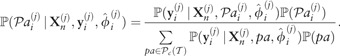
Given a set of d datasets collected in d species (for notational simplicity, we assume one dataset per species, with a shared indexing, i.e. dataset i always corresponds to species i; this need not be true in general and multiple datasets can be collected in a given species), denoted where represents the data in species i (a superscript is used throughout to denote dataset/species index), the aim is to infer a set of GRNs, one for each of the d species , where the networks may be similar but not necessarily identical. Here, the ith GRN denotes a directed graph for species i with nodes , edges and node labels , where node labels can be assigned according to the set of orthologues each node has, either based on manually curated lists, or else through sequence similarity. Within the first model, a hypernetwork, which must also be inferred, is used to constrain the individual networks in the different species, and is denoted , and has one node for each of the unique node labels across the d species. The posterior distribution over networks is given by
| (1) |
Here, β represents any free parameters in the joint prior distribution over network structures, . The term represents the probability of observing the jth dataset conditional on network and model parameters , with used to denote a likelihood and a normalizing constant. The exact form of these data models, , will depend on the type of data available. For time series gene expression data, suitable models include the Gaussian process approach (Äijö and Lähdesmäki, 2009; Klemm, 2008; Penfold and Wild, 2011; Penfold et al., 2012) as outlined in Section 2.4, or linear regression approaches (Oates et al., 2014). Other models will be appropriate when dealing with different types of data such as the use of Bayesian networks for collections of steady-state gene expression data, in which case we would additionally require the individual networks be directed acyclic graphs. A joint prior distribution over network structures is chosen to correspond to a Gibbs distribution:
| (2) |
where represents an energy function capturing dissimilarities between networks and a normalizing constant arising from the prior distribution over network structures. The parameter β effectively controls the strength of influence of each of the individual networks on the hypernetwork and vice versa: for , the model recovers independent fitting to each of the species given the species-specific data, while very large values of β increasingly favour similar networks. From the hierarchical structure of the model in Figure 1a, it is clear that the GRNs are conditionally independent of one another given the hypernetwork, and the joint prior becomes
| (3) |
Within this framework, each dataset may possess a different value for β, although here we concentrate on the case . In the previous work (Oates et al., 2014; Penfold et al., 2012; Werhli and Husmeier, 2008), network dissimilarity was measured using the structural Hamming distance between network j and the hypernetwork, denoted . That is, the energy associated with two networks is proportional to the distance between them, as represented by a count of the number of times the edges in the two networks disagree. Here, we instead quantify similarity between two networks using a graph kernel, , which naturally allows us to capture the similarity between graphs even where duplicate nodes exist, and can readily quantify more complex similarities in the networks that may be missed when using the structural Hamming distance (see Section 2.3). Because we are now capturing network similarity, rather than dissimilarity, we may take the following:
| (4) |
where represents a similarity measure between two graphs and represents the maximal similarity score possible, and increasing the value of the parameter β acts to constrain the networks across species to favour increasing similar structures, if possible. Nevertheless, if the networks are also informed by species-specific time series datasets, this should allow the model to identify correct network structures even when, for example, orthologues have been mislabelled, provided enough data exist. Consequently, this approach should be able to identify common aspects, increasing the overall accuracy of network reconstruction, while still allowing the GRNs to possess species-specific embellishments.
When β and are fixed, JI proceeds via a series of Gibbs updates to the parental set of each of the nodes in each of the networks and hypernetwork in turn (Supplementary Section S1). In some model organisms, high-throughput yeast one-hybrid or ChIP-Seq experiments have elucidated large sections of the GRNs, and a special case of JI exists, in which the known network is fixed, allowing information to be leveraged into other species. It is this special case that is refered to as “NL” (Supplementary Materials Section S1.1).
2.2 Framework 2: direct leveraging of orthologous networks
When leveraging network information directly between species as indicated in Figure 1b, we have the following posterior distribution over GRNs and model parameters:
| (5) |
where all terms are as previously described. To recap, and represent the data and network in species j, with denoting hyperparmeters in the data model, and β denoting parameters in the joint prior distribution over networks. Here, the prior distribution over network structures is again assumed to correspond to a Gibbs distribution [Equation (2)], where the energy is calculated as the pairwise contribution from all networks:
| (6) |
where . From Figure 1b, it is apparent that the main difference here, compared with the previous framework, is that the networks are no longer conditionally independent of one another given a hypernetwork. That is, each network directly influences each other network through a joint prior. For fixed β and , JI can proceed via a series of Gibbs updates of the parental sets of each node in each species (Supplementary Section S1), while NL can be approached by fixing the topology of any network, allowing the propagation of information from that species to all others.
2.3 Network similarity via graph kernels
The models outlined in Sections 2.1 and 2.2 rely on our ability to evaluate how similar or dissimilar two graphs are. Here, we chose to do so via graph kernels, which, informally, represent a function of two graphs that quantifies their similarity (Shervashidze et al., 2011). Graph kernels fall broadly into three categories: (i) those based on similarities of the walks and paths in the respective graphs; (ii) those based on similarities in limited-sized subgraphs and (iii) those based on sub-tree patterns. We use an example of each of the three types of graph kernel, discussed below:
- • Shortest path graph kernel: For two graphs and , we may first calculate the shortest path graphs and , with the shortest path graph kernel defined as:
where represents a positive definite kernel over walks of length 1, that is, over edges in the shortest path graphs. If edges in the graphs are unweighted, a Dirac delta function may be used, that is, we may sum over all edges in the respective networks with if the edges match and 0 otherwise. Here, for labelled graphs, edges are considered as matching if they both connect a node with label l with a node with label m. See also Borgwardt and Kriegel (2005).
• Graphlet kernels: The similarity between two graphs may be evaluated by first decomposing each graph into limited-size graphlets. The k-spectrum is defined as the vector containing the count of each of the different graphlets of size k in . Given a second graph , the similarity between the two graphs can be evaluated as follows:
(7) When the two graphs vary in size, the counts may be heavily skewed. Here, the k-spectrum may be normalized to frequency, , where is the total number of graphlets in . We then have . See also Supplementary Figure S1 and Shervashidze et al. (2009, 2011).
• Weisfeiler–Lehman (WL) kernel: The WL kernel evaluates the similarity between two graphs by comparing sub-tree patterns (Shervashidze et al., 2011). Specifically, the node in the respective graph is re-labelled according to which nodes they are connected to. For example, the nodes in the initial graph, denoted , may be re-labelled according to neighbours of each node to generate a new graph . Here, the nodes and edges are conserved, but the updated labels contain information about the immediate neighbourhood of each node. The hth round of re-labelling generates the graph . For an h-step WL kernel, we thus have the sequence of graphs and the WL kernel may be evaluated as follows:
(8) where represents a positive definite base kernel. We use h = 2 throughout, and an illustrative example for a two-step WL kernel is included in Supplementary Figure S2.
In general, graphs that are similar will have higher scores than graphs that are different. Although the three graph kernels tested in this study were all designed for labelled graphs, this need not be the case in general, and a significant number of graph kernels exist for quantifying the similarity or dissimilarity between unlabelled graphs. The use of labelled graphs within this context could be considered advantageous, because it allows us to encode the assumption that orthologues should be regulated by genes that themselves are orthologous. Here, the assignment of labels may be done using manually curated lists or BLAST reciprocal best hits.
2.4 Gaussian process model for gene expression
Within this article, we will deal exclusively with time series data, and therefore use the Gaussian process model outlined by Klemm (2008), which has been shown to outperform many state-of-the-art approaches on a range of in silico and biological benchmarks (Hickman et al., 2013; Penfold and Wild, 2011; Penfold et al., 2012). For this model, the dynamics of a gene i in species j evolve as follows:
| (9) |
where denotes the expression level of gene i in dataset j at time t, the expression of all genes in the system at time t, represents the parents of gene i in dataset j, ε represents some (Gaussian) observational noise (that may be dataset specific) and indicates an unknown non-linear function specific to dataset j. Because of the nature of the model, we may split the data into an input, , and output, , set of data as follows:
where and represent the number of genes and time series observation in species j. Here, we assign the unknown function a Gaussian process prior (Rasmussen and Williams, 2006), denoted by , and may analytically calculate the probability of observing the output for gene i, , conditional on the parental set and observations :
Under a Gaussian noise model, this integral is analytically tractable, and we thus have , where represents a vector of zeros of length and represents an identity matrix (Rasmussen and Williams, 2006). Here, represents the hyperparameters of the Gaussian process prior, the interpretation of which will depend on the choice of covariance function. In this case, as with previous works (Penfold and Wild, 2011; Penfold et al., 2012), the functional form of the covariance function was chosen to be the squared exponential and the hyperparameters represent the standard deviation of the observation noise, standard deviation of the process and characteristic length scale, node i in species j. The parents of a given gene are not known a priori however, but are learnt via Bayes’ rule:
 |
where denotes the truncated power set of putative regulators/transcription factors for gene i in dataset j. That is, we only consider combinations of regulators up to maximum cardinality c, where we use c = 2 throughout. Although this imposes a limit on the maximum number of genes that can regulate another simultaneously, no such limits exist in the networks derived from the marginal probabilities for regulation, which can be calculated from the full joint distribution. Finally, the hyperparameters may be estimated by maximizing
Within this framework, the probability for each parental set may therefore be pre-computed for each of the individual species, alongside an estimation of , which may be substituted directly into Equations (1) and (5).
3 Results
In Sections 3.1 and 3.2, we characterize the performance of the Orthologous Causal Structure Identification (OCSI) algorithm on in silico benchmarks for which there are known gold standards and compare with the Causal Structure Identification (CSI) algorithm (Penfold and Wild, 2011). In Section 3.3, we use OCSI to leverage cell cycle networks from S.cerevisiae into S.pombe, and also perform JI in both species.
3.1 In silico networks with 1:1 mapping of nodes
The OCSI algorithm was initially tested using dataset 5 from the DREAM4 10-gene network challenge. This dataset consist of five time series generated under five different conditions from an identical network. Because these networks are identical, this benchmark does not test inference in multiple species with duplicate nodes (it should be noted, however, that the dynamics in each of the five time series are perturbed, and this situation might therefore reflect inference using closely related species in which the underlying network has been conserved). Nonetheless, this benchmark is an important case that establishes any initial advantages that might exist, compared with stand-alone inference, and allows us to gauge how different graph kernels behave within the context of network inference. In general, the use of hierarchical modelling allows more accurate reconstruction of networks than standalone inference (Bourque and Sankoff, 2004; Oates et al., 2014; Penfold et al., 2012; Wang et al., 2006), and the same appears to be true for OCSI, with the WL kernel performing better than the other graph kernels tested. Furthermore, the hierarchical model/Framework 1 appeared to be more stable when many datasets were used, with the non-hierarchical model/Framework 2 more stable when fewer datasets were considered. Full details about initial benchmarking are included in Supplementary Section S2.
3.2 In silico networks with duplicate nodes
A second set of in silico data was used to benchmark the performance of OCSI, this time on networks that contain duplicate nodes. These datasets represented five species that are related as shown in Figure 2a. A core network in species A was modelled based on the repressilator (Elowitz and Leibler, 2000); a second species B has an identical network structure as species A, but the dynamics have been perturbed. Duplication of the repressilator network of species A resulted in an intermediate species I, which is not observed. Subsequent loss of nodes, loss of connections and a perturbation of dynamics in species I resulted in species C. Species D also derives from species I via loss of edges, and finally species E is derived from species D via a perturbation of the dynamics. For each species, a time series of messenger RNA (mRNA) expression was generated consisting of 21 time points, as shown in Figure 2b. Full details of the models, including information about data generation, can be found in Supplementary Section S3. Benchmarking of the OCSI algorithm was undertaken as follows: (i) a five species case, in which mRNA time series are observed for species A through E inclusive (species I is not observed); (ii) a two species case, in which mRNA time series are observed for species C and D and (iii) a two species case in which the network in either species A or C is known and fixed, and inference of the network of species D is undertaken by jointly leveraging the network of species A/C alongside time series mRNA expression data of species E. For the five species case, the area under the receiver operating characteristic curve (AUC) for the various species is shown for the WL graph kernel in Figure 2c–e, where dashed (red) lines indicate the AUC under stand-alone inference, and solid (blue) lines indicate AUC as a function of β for the two OCSI frameworks outlined in this article. The top row indicates performance when network information is directly leveraged (Framework 2), while the bottom row indicates performance when information is leveraged via a hypernetwork (Framework 1). The average AUC over all 5 species as a function of β is shown in Figure 2d, while the marginal likelihood at various values of β is shown in Figure 2e. When β is small, accuracy of OCSI corresponds to that found using stand-alone inference, as expected. For intermediate values of β (over the range tested), OCSI improves the accuracy of reconstructed networks, particularly in species B, C and E, where AUC has increased from in the stand-alone inference to in Framework 1 and in Framework 2. For species D, reconstruction from the time series data is already nearly perfect (), but nonetheless some increase in AUC is observed, with a value of 0.89 in Framework 1 and 0.91 in Framework 2. For species A, in which the network has been reconstructed from time series data with , the performance of OCSI at intermediate values of β remains 1, indicating that there is no degradation in network reconstruction in species for which the data are highly informative. As β increases further, performance begins to degrade, both in terms of accuracy as measured by the AUC, and in terms of increased variance in the estimated AUC of multiple Markov Chain Monte Carlo (MCMC) runs. A similar trend is seen for the average AUC as a function of β, that is, the AUC averaged over all five species shows initially increases from 0.79 to 0.95 in both frameworks before degrading at higher values of β. For Framework 1, in which information is propagated via an hypernetwork, the peak performance occurs at approximately β = 3, while for Framework 2, in which information is directly propagated between species, peak performance occurs at approximately β = 1. In this case, Framework 1 appears to be more stable than Framework 2, that is, the range of β over which the algorithm yields improved AUC compared with standalone inference is greater, suggesting that, in cases where the normalizing constant cannot be computed and β must be set arbitrarily, Framework 1 may be more useful. In our example, we were able to estimate the marginal likelihood (Supplementary Section S1.3), which is indicated in Figure 2e. Here, the value of β that corresponds to the greatest marginal likelihood corresponds well to the region in which the AUC is highest. Performance of the graphlet kernel and shortest path graph kernels did not appear to be considerably better than standalone inference over the range of β tested (data not shown).
Fig. 2.

(a) Relationships between species. The network in species A is represented by the repressilator. Species B evolved from A, conserving the general architecture of the repressilator but with the underlying dynamics perturbed. Species I evolved from A via a duplication of the repressilator. Species C evolved from species I via loss of a node, loss of edges and perturbation of the dynamics. Species D evolved from species I via loss of edges. Species E evolved from D via a perturbation of the dynamics. (b) Simulated mRNA time series for the five species. (c) AUC for the five species using the non-hierarchical/Framework 2 (top) and hierarchical/Framework 1 (bottom) versus β. (d) AUC averaged over all species versus β. (e) Estimated marginal likelihood versus β
For the two species case, the AUC is shown in Supplementary Figure S7b–d. Here, networks were reconstructed using species C and D. As with the five species case, the AUC for small values of β corresponded well to standalone inference in both frameworks. For species C, as β increased, the AUC increased from 0.59 in the standalone inference to 0.96 in Framework 1 and 0.98 in Framework 2. Because species D already had good reconstruction accuracy from the time series data alone, further improvements may not have been expected. Nonetheless, a small increase in AUC was seen, rising from 0.86 in the standalone inference to 0.89 in Framework 1 and 0.88 in Framework 2. Overall, the average AUC rose from 0.72 in standalone inferences to 0.91 and 0.92 in Frameworks 1 and 2, respectively (Supplementary Figure S7c). As with the five dataset case, if β was increased too much the accuracy of the algorithms began to diminish, with AUC falling and increasingly varied, suggesting that for high values of β exploration of the parameter space may be difficult, with chains becoming stuck in suboptimal modes. For the two dataset case, Framework 2 appeared to be more stable than Framework 1, that is, the range over β in which the performance is greater than standalone was larger in Framework 2 than it was in Framework 1. Estimation of the marginal likelihood (Supplementary Figure S7d) suggests that the region in which the marginal likelihood was greatest corresponds well to the values of β for which the AUC was highest. Performance of the graphlet kernel and shortest path graph kernels did not appear to be considerably better than standalone inference over the range of β tested (data not shown).
Finally, OCSI was used to jointly leverage network information from one species, alongside time series gene expression data from another. Here, we used two examples, in the first instance the network in species A was assumed to be known, and was thus fixed, and leveraged into species E, alongside time series data for species E. In the second example, the network C was assumed to be known, and was thus fixed and leveraged into species E. The performance in terms of reconstruction of the network in species E when the network in A was fixed is shown as a function of β in Supplementary Figure S8, with the accuracy in the reconstruction of network E when species C’s GRN is fixed as shown in Supplementary Figure S9. In both cases, the accuracy of network reconstruction in species E (in terms of AUC) increased from 0.71 in the standalone inference to in Framework 1 and Framework 2, respectively, when GRN of species A is fixed, and to 0.96 in both frameworks when the GRN of species C was fixed. In all cases, the AUC was optimal or near optimal when the marginal likelihood was greatest. However, inference in the non-hierarchical framework appeared to be more stable over a greater range of β than the hierarchical version, suggesting that when normalizing constant could not be estimated, direct leveraging of networks from model organisms to more relevant ones is best approached with Framework 2.
3.3 Leveraging cell cycle networks in yeast
We have applied OCSI to infer cell cycle networks in S.pombe, for which the GRN is less well characterized than S.cerevisiae. Here, we use OCSI Framework 2 to perform three types of inference: (i) in the first instance, the GRN of S.cerevisiae was directly propagated to S.pombe utilizing graph kernels, that is, without utilizing any time series data, effectively representing samples from the prior distribution; (ii) in the second instance, the S.cerevisiae network was utilized alongside S.pombe time series to infer an S.pombe cell cycle network, that is, an NL task and (iii) in the third instance, time series from both species were used to perform JI, with the S.cerevisiae network used as a prior. This inference is represented graphically in Supplementary Figure S10. Genes and regulatory connections involved in the S.cerevisiae cell cycle were identified from Li et al. (2004) and used to construct a fixed S.cerevisiae network, with genes involved in the S.pombe cell cycle identified from Bushel et al. (2009). Additional genes were introduced into both lists based on the manually curated orthologue list of PombBase (Wood et al., 2012). In total, 157 genes were identified for S.cerevisiae with 165 connections between them and 100 genes for S.pombe. These genes included 17 duplicated genes, 7 S.cerevisiae-specific nodes and 53 S.pombe-specific nodes (full lists of genes can be found for S.cerevisiae and S.pombe in Supplementary Files S1 and S2, respectively). The S.pombe transcriptional time series data were taken from Rustici et al. (2004) and S.cerevisiae time series taken from Cho et al. (1998), Spellman et al. (1998), Pramila et al. (2006) and Granovskaia et al. (2010).
Approximately 60% of the top 100 connections were common between the JI and NL approaches, with around 50% of the top 1000 connections in common, suggesting broad agreement between the two approaches. Although literature connections for S.pombe are less well documented than for S.cerevisiae, some known connections were found using BioGRID (Stark et al., 2006), while predicted S.pombe protein interactions could be found in Pancaldi et al. (2012), and were used to evaluate preliminary performance of all three runs (Supplementary Table S1). In general, the agreement between inferred networks and available literature was relatively low (∼ represented true positives), reflecting the fact that less is known about the S.pombe cell cycle network than the S.cerevisiae network. Indeed, the ground truth connections used here may not represent casual or direct interactions that we are attempting to infer here, and any lack of agreement should therefore be interpreted with caution. Nonetheless, the JI of networks and NL approaches yielded greater agreement than expected by chance, and additionally appeared to have greater agreement with the literature than when we directly leverage the S.cerevisiae network into S.pombe using graph kernels without using additional time series data.
OCSI was able to capture several important regulatory links among the S.pombe cell cycle genes. In S.pombe, the MCB-binding factor transcription complex (where MCB is Mlu1 Cell cycle Box), which contains the Cdc10, Res1 and Res2 proteins, is responsible for the cell cycle-regulated transcription of many genes during G1 phase of the cell cycle (Bertoli et al., 2013). Genes that are regulated by the MBF complex include G1 cyclins (Cig2), proteins required for loading the mini-chromosome maintenance helicase to DNA replication origins (Cdc18 and Cdt1) and cell cycle-regulated transcription factors (Yox1 and Tos4). Our data recapitulate many of the known interactions and dependencies identified previously by others (full networks available in Supplementary Files S4–S6). In addition, both JI and NL identify Gas1 as a cell cycle-regulated gene involved in the transcription of MBF-regulated genes, including Mrc1, Cdt2, Rad21, Msh6 (Figure 3), as well as a variety of other genes, representing one of the most highly connected hubs. Gas1 is a 1,3-beta-glucanosyltransferase that elongates and rearranges 1,3-beta-glucan side chains, which are cross-linked with 1,6-beta-glucan, chitin and proteins to form the main layer of the cell wall (Mouyna et al., 2000; Ragni et al., 2007). In budding yeast, cells lacking Gas1 have weakened and abnormal cell walls and are sensitive to cell wall-perturbing drugs. Recently, however, a surprising new role for Gas1 activity has been identified in the regulation of transcriptional silencing at rDNA loci (Eustice and Pillus, 2014; Ha et al., 2014; Koch and Pillus, 2009). In particular, it has been suggested that Gas1 physically interacts with Sir2, an nicotinamide adenine dinucleotide (NAD)+-dependent histone deacetylase that is a subunit of the rDNA silencing complex (RENT: regulator of nucleolar silencing and telophase exit), to repress Pol II-dependent transcription at the rDNA locus (Huang and Moazed, 2003). The observations that in budding yeast a pool of Gas1 both localizes to the nuclear periphery (Huh et al., 2003) and interacts with other diverse components of the chromatin modifying machinery (www.thebiogrid.org) support a role for Gas1 in transcriptional regulation. One possibility is that Gas1 may interact physically with the MBF complex to mediate cell cycle-regulated transcription of MBF-regulated genes or a subset of those genes that are involved in cell wall biogenesis in fission yeast. Further experiments will be needed to test this possibility.
Fig. 3.
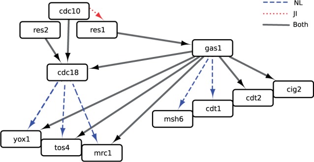
A small sub-network of the Schizosaccharomyces pombe cell cycle network inferred using OCSI (Framework 2). This network was able to recapitulate known aspects of the S.pombe cell cycle network including relationships among Res1 (SPBC725.16), Res2 (SPAC22F3.09c), Cdc10 (SPBC336.12c), Yox1 (SPBC21B10.13c), Tos4 (SPAP14E8.02) and Mrc1 (SPAC694.06c), and predicts a novel role for Gas1 (SPAC19B12.02c) as a key regulator of Yox1, Tos4(SPAP14E8.02), Mrc1, Cig2 (SPAPB2B4.03), Cdt1(SPBC428.18), Cdt2 (SPBC11B10.09) and Msh6 (SPCC285.16c), among others. Here, we also indicate if connections were found from NL (dashed edges), JI (dotted edges) or both (solid edges)
4 Discussion
Deciphering complex biological networks and elucidating how those networks influence emergent properties increasingly rely on piecing together many diverse sets of experimental data. The ability to leverage data from several related species is particularly desirable, and would allow the vast amount of information obtained in model organisms to be translated into more medically or economically relevant ones. Possible applications include the joint learning of GRNs associated with disease progression in mice and humans, or the direct leveraging of networks associated with seed yield, seed quality, stress tolerance or resistance that have been constructed in the model plant Arabidopsis into crops. Despite the underlying similarities in the GRNs of closely related species, however, significant evolutionary differences may still exist that can confound standard approaches to inferring GRNs from large-scale transcriptomics data. Here, we have developed two Bayesian approaches to network inference that allow for such leveraging of interspecies data. These models perform better than a related approach on in silico benchmarks, and are robust to small amounts of orthologue mislabelling and to gene duplication. We have also successfully used them to leverage information about the S.cerevisiae cell cycle network into S.pombe, and also performed JI between S.cerevisiae and S.pombe. Our analysis of the networks in S.pombe showed some agreement with the literature, although the true positive rate was relatively low, perhaps reflecting that the ‘gold standard’ networks we used did not necessarily contain many direct interactions. Nonetheless, our method identified a number of known key cell cycle interactions and predicted a novel role for Gas1 (SPAC19B12.02c) in cell cycle activities.
The methods outlined here share many of the same principles as earlier works (Zhang and Moret, 2010). Our methods, however, rely on graph kernels to capture the similarity between labelled graphs, rather than explicit evolutionary models. Broadly speaking, the labelling procedure requires that nodes to be assigned to groups, which can be informed by manually curated lists of orthologues, or on the basis of sequence similarity (Kashima et al., 2009). Because the networks are additionally informed by time series data, the method is robust to some mislabelling of nodes, although more adaptive procedures can be envisaged in which node labels are assigned, or refined, within the inference procedure (Gholami and Fellenberg, 2010). In general, there is no explicit requirement to use labelled graph kernels, although doing so represents an effective way of encoding biological expectations that orthologues function similarly between species. Graph kernels for unlabelled graphs do exist, and could be used within OCSI, which would favour similar structures between the networks as a whole, without placing any implicit restraints on where a given node belongs with respect to the others: that is, the joint prior in the method would favour similar network properties rather than similar biological positioning. One possible future line of work could focus on combining labelled and unlabelled graph kernels for situations in which only smaller sets of orthologues can be identified. The diversity of graph kernels, however, may be problematic, as it is not immediately clear which graph kernels yield the best results for a given situation. Here, we have used three different graph kernels, with the WL kernel appearing to offer better performance than the graphlet and shortest path kernels overall. It is not currently clear why this might be, although one possibility is that the graphlet and shortest path kernels are not suited to the small or densely connected networks we used for benchmarking. Alternatively, the choice of β for the shortest path and graphlet kernels may be inappropriate. Future approaches might therefore look to address how to tune β automatically within the algorithm as in Penfold et al. (2012). It has been noted, however, that at high values of β, the MCMC procedure, that is, a Gibbs update of the parental set of each node in turn, begins to fail due to the high modality in the parameter space. To develop approaches that can tune β, more advanced MCMC algorithms will be needed (Calderhead and Girolami, 2009). Alternatively, another promising approach would be to automatically combine multiple graph kernels together allowing for increased flexibility in characterizing network similarity, albeit at additional computational costs.
Finally, as well as the flexibility conferred on the inference process by using graph kernels, our approach allows the possibility of exploiting other properties of graph kernels. Because the graph kernels we have used are positive semi-definite, this will allow algorithms that not only jointly infer networks over species, but also tie those networks to phenotypic observations via a separate Gaussian process model utilizing the graph kernels as a covariance function.
Funding
This work was supported by the Engineering and Physical Sciences Research Council (EPSRC) grants EP/I036575/1, EP/J020281/1 and Biotechnology and Biological Sciences Research Council (BBSRC) grant BB/F005806/1. J.B.A.M. is supported by a programme grant (MR/K001000/1) from the Medical Research Council (MRC), UK. This research utilized Queen Mary’s MidPlus computational facilities, supported by Queen Mary University of London-IT and funded by EPSRC grant EP/K000128/1.
Conflict of Interest: none declared.
Supplementary Material
References
- Äijö T., Lähdesmäki H. (2009) Learning gene regulatory networks from gene expression measurements using non-parametric molecular kinetics. Bioinformatics, 25, 2937–2944. [DOI] [PubMed] [Google Scholar]
- Bertoli C., et al. (2013) Control of cell cycle transcription during G1 and S phases. Nat. Rev. Mol. Cell Biol., 14, 518–528. [DOI] [PMC free article] [PubMed] [Google Scholar]
- Borgwardt K.M., Kriegel H.P. (2005) Shortest-path kernels on graphs. In Proceedings of the International Conference on Data Mining. IEEE Computer Society, Washington, DC, USA, pp. 74–81. [Google Scholar]
- Boto L. (2010) Horizontal gene transfer in evolution: facts and challenges. Proc. R. Soc. B, 277, 819–827. [DOI] [PMC free article] [PubMed] [Google Scholar]
- Bourque G., Sankoff D. (2004) Improving gene network inference by comparing expression time-series across species, developmental stages or tissues. J. Bioinform. Comput. Biol., 2, 765–783. [DOI] [PubMed] [Google Scholar]
- Breeze E., et al. (2011) High-resolution temporal profiling of transcripts during Arabidopsis leaf senescence reveals a distinct chronology of processes and regulation. Plant Cell, 23, 873–894. [DOI] [PMC free article] [PubMed] [Google Scholar]
- Bushel P.R., et al. (2009) Dissecting the fission yeast regulatory network reveals phase-specific control elements of its cell cycle. BMC Syst. Biol., 3, 93. [DOI] [PMC free article] [PubMed] [Google Scholar]
- Calderhead B., Girolami M.A. (2009) Estimating Bayes factors via thermodynamic integration and population MCMC. Comput. Stat. Data Anal., 53, 4028–4045. [Google Scholar]
- Carvunis A.R., et al. (2012) Proto-genes and de novo gene birth. Nature, 487, 370–374. [DOI] [PMC free article] [PubMed] [Google Scholar]
- Cho R.J., et al. (1998) A genome-wide transcriptional analysis of the mitotic cell cycle. Mol. Cell, 2, 65–73. [DOI] [PubMed] [Google Scholar]
- Clark C., Kalita J. (2014) A comparison of algorithms for the pairwise alignment of biological networks. Bioinformatics, 30, 2351–2359. [DOI] [PubMed] [Google Scholar]
- Elowitz M.B., Leibler S. (2000) A synthetic oscillatory network of transcriptional regulators. Nature, 403, 335–338. [DOI] [PubMed] [Google Scholar]
- Eustice M., Pillus L. (2014) Unexpected function of the glucanosyltransferase Gas1 in the DNA damage response linked to histone H3 acetyltransferases in Saccharomyces cerevisiae. Genetics, 196, 1029–1039. [DOI] [PMC free article] [PubMed] [Google Scholar]
- Gholami A.M., Fellenberg K. (2010) Cross-species common regulatory network inference without requirement for prior gene affiliation. Bioinformatics, 26, 1082–1090. [DOI] [PubMed] [Google Scholar]
- Granovskaia M.V., et al. (2010) High-resolution transcription atlas of the mitotic cell cycle in budding yeast. Genome Biol., 11, R24. [DOI] [PMC free article] [PubMed] [Google Scholar]
- Ha C.W., et al. (2014) The β-1,3-glucanosyltransferase Gas1 regulates Sir2-mediated rDNA stability in Saccharomyces cerevisiae. Nucleic Acids Res., 42, 8486–8499. [DOI] [PMC free article] [PubMed] [Google Scholar]
- Hickman R., et al. (2013) A local regulatory network around three NAC transcription factors in stress responses and senescence in Arabidopsis leaves. Plant J., 75, 26–39. [DOI] [PMC free article] [PubMed] [Google Scholar]
- Hisgett T. (2012) Golden Eagle 2a. http://www.flickr.com/photos/hisgett/6022378177/ (8 May 2015, date last accessed). [Google Scholar]
- Huang J., Moazed D. (2003) Association of the RENT complex with nontranscribed and coding regions of rDNA and a regional requirement for the replication fork block protein Fob1 in rDNA silencing. Genes Dev., 17, 2162–2176. [DOI] [PMC free article] [PubMed] [Google Scholar]
- Huh W.K., et al. (2003) Global analysis of protein localization in budding yeast. Nature, 425, 686–691. [DOI] [PubMed] [Google Scholar]
- Joshi A., et al. (2014) Multi-species network inference improves gene regulatory network reconstruction for early embryonic development in Drosophila. ArXiv preprint arXiv:1407.6554. [DOI] [PubMed] [Google Scholar]
- Kashima H., et al. (2009) Simultaneous inference of biological networks of multiple species from genome-wide data and evolutionary information: a semi-supervised approach. Bioinformatics, 25, 2962–2968. [DOI] [PubMed] [Google Scholar]
- Klemm S.L. (2008) Causal structure identification in nonlinear dynamical systems. MPhil Thesis, Department of Engineering, University of Cambridge, Cambridge, UK. [Google Scholar]
- Koch M.R., Pillus L. (2009) The glucanosyltransferase Gas1 functions in transcriptional silencing. Proc. Natl. Acad. Sci. USA, 106, 11224–11229. [DOI] [PMC free article] [PubMed] [Google Scholar]
- Lersch T. (2005) Common Chimpanzee in the Leipzig zoo. http://upload.wikimedia.org/wikipedia/commons/6/62/Schimpanse_Zoo_Leipzig.jpg (8 May 2015, date last accessed). [Google Scholar]
- Li F., et al. (2004) The yeast cell-cycle network is robustly designed. Proc. Natl. Acad. Sci. USA, 101, 4781–4786. [DOI] [PMC free article] [PubMed] [Google Scholar]
- Logan A. (2003) Laboratory mice. http://www.lightmatter.net/ (8 May 2015, date last accessed). [Google Scholar]
- Mouyna I., et al. (2000) Glycosylphosphatidylinositol-anchored glucanosyltransferases play an active role in the biosynthesis of the fungal cell wall. J. Biol. Chem., 275, 14882–14889. [DOI] [PubMed] [Google Scholar]
- Mueller J. (2007) Rob Paulsen and Maurice LaMarche at the 2006 Annie Awards red carpet at the Alex Theatre in Glendale, California. https://upload.wikimedia.org/wikipedia/commons/8/83/Annie_Awards_Rob_paulsen_and_maurice_lamarche.jpg (8 May 2015, date last accessed). [Google Scholar]
- Oates C.J., et al. (2014) Joint estimation of multiple related biological networks. Ann. Appl. Stat., 8, 1892–1919. [Google Scholar]
- Pancaldi V., et al. (2012) Predicting the fission yeast protein interaction network. G3 (Bethesda) , 2, 453–467. [DOI] [PMC free article] [PubMed] [Google Scholar]
- Penfold C., et al. (2012) Nonparametric Bayesian inference for perturbed and orthologous gene regulatory networks. Bioinformatics, 28, i233–i241. [DOI] [PMC free article] [PubMed] [Google Scholar]
- Penfold C.A., Wild D.L. (2011) How to infer gene networks from expression profiles, revisited. J. R. Soc. Interface Focus, 6, 857–870. [DOI] [PMC free article] [PubMed] [Google Scholar]
- Pramila T., et al. (2006) The Forkhead transcription factor Hcm1 regulates chromosome segregation genes and fills the S-phase gap in the transcriptional circuitry of the cell cycle. Genes Dev., 20, 2266–2278. [DOI] [PMC free article] [PubMed] [Google Scholar]
- Ragni E., et al. (2007) The gas family of proteins of Saccharomyces cerevisiae: characterization and evolutionary analysis. Yeast, 24, 297–308. [DOI] [PubMed] [Google Scholar]
- Rasmussen C., Williams C.K.I. (2006) Gaussian Processes for Machine Learning. 2nd edn MIT Press, Cambridge, MA, USA. [Google Scholar]
- Rustici G., et al. (2004) Periodic gene expression program of the fission yeast cell cycle. Nat. Genet., 36, 809–817. [DOI] [PubMed] [Google Scholar]
- Shervashidze N., et al. (2009) Efficient graphlet kernels for large graph comparison. In Proceedings of the Twelfth International Conference on Artificial Intelligence and Statistics (AISTATS 2009), Vol. 5, pp. 488–495. [Google Scholar]
- Shervashidze N., et al. (2011) Weisfeiler-Lehman graph kernels. J. Mach. Learn. Res., 12, 2539–2561. [Google Scholar]
- Soltis P.S., Soltis D.E. (2009) The role of hybridization in plant speciation. Annu. Rev. Plant Biol., 60, 561–588. [DOI] [PubMed] [Google Scholar]
- Spellman P.T., et al. (1998) Comprehensive identification of cell cycle-regulated genes of the yeast Saccharomyces cerevisiae by microarray hybridization. Mol. Biol. Cell, 9, 3273–3297. [DOI] [PMC free article] [PubMed] [Google Scholar]
- Stark C., et al. (2006) Biogrid: a general repository for interaction datasets. Nucleic Acids Res., 34(Database issue), D535–D539. [DOI] [PMC free article] [PubMed] [Google Scholar]
- Steveoc86. (2011) Artist's impression of an individual in brooding position. http://upload.wikimedia.org/wikipedia/commons/e/ed/Deinonychus_Steveoc.jpg (8 May 2015, date last accessed).
- Towfic F., et al. (2009) Aligning biomolecular networks using modular graph kernels. In: Proceedings of the 9th International Conference on Algorithms in Bioinformatics , Springer, pp. 345–361. [Google Scholar]
- Wang Y., et al. (2006) Inferring gene regulatory networks from multiple microarray datasets. Bioinformatics, 22, 2413–2420. [DOI] [PubMed] [Google Scholar]
- Werhli A.V., Husmeier D. (2008) Gene regulatory network reconstruction by Bayesian integration of prior knowledge and/or different experimental conditions. J. Bioinform. Comput. Biol., 6, 543–572. [DOI] [PubMed] [Google Scholar]
- Windram O., et al. (2012) Arabidopsis defense against Botrytis cinerea: chronology and regulation deciphered by high-resolution temporal transcriptomic analysis. Plant Cell, 24, 3530–3557. [DOI] [PMC free article] [PubMed] [Google Scholar]
- Wood V., et al. (2012) PomBase: a comprehensive online resource for fission yeast. Nucleic Acids Res., 40(Database issue), D695–D699. [DOI] [PMC free article] [PubMed] [Google Scholar]
- Zhang X., Moret B.M. (2010) Refining transcriptional regulatory networks using network evolutionary models and gene histories. Alg. Mol. Biol., 5, 1. [DOI] [PMC free article] [PubMed] [Google Scholar]
- Zhao G., et al. (2013) Inferring regulatory networks through orthologous gene mapping. In: Proceedings of the IEEE International Conference on Bioinformatics and Biomedicine, Shanghai, 18–21 December 2013. IEEE, pp. 76–83. [Google Scholar]
Associated Data
This section collects any data citations, data availability statements, or supplementary materials included in this article.