

Abstract
A number of biomedical problems require performing many hypothesis tests, with an attendant need to apply stringent thresholds. Often the data take the form of a series of predictor vectors, each of which must be compared with a single response vector, perhaps with nuisance covariates. Parametric tests of association are often used, but can result in inaccurate type I error at the extreme thresholds, even for large sample sizes. Furthermore, standard two-sided testing can reduce power compared with the doubled  -value, due to asymmetry in the null distribution. Exact (permutation) testing is attractive, but can be computationally intensive and cumbersome. We present an approximation to exact association tests of trend that is accurate and fast enough for standard use in high-throughput settings, and can easily provide standard two-sided or doubled
  -values. The approach is shown to be equivalent under permutation to likelihood ratio tests for the most commonly used generalized linear models (GLMs). For linear regression, covariates are handled by working with covariate-residualized responses and predictors. For GLMs, stratified covariates can be handled in a manner similar to exact conditional testing. Simulations and examples illustrate the wide applicability of the approach. The accompanying mcc package is available on CRAN http://cran.r-project.org/web/packages/mcc/index.html.
Keywords: Density approximation, Exact testing, Permutation
1. Introduction
High-dimensional datasets are now common in a variety of biomedical applications, arising from genomics or other high-throughput platforms. A standard question is whether a clinical or experimental variable (hereafter called the response) is related to any of a potentially large number of predictors. We use  to denote the response vector of length
  (random vector
  , observed elements
  ), and
  to denote the
  matrix of predictors. Standard analysis often begins by testing for association of
  vs. each row
  of
of  , i.e. computing a statistic
  for each hypothesis
  . The most common corrections for multiple testing, such as Benjamini–Hochberg false discovery rate control, require only individual
  -values for the
  test statistics. Thus, at the level of a single hypothesis, the role of
  is to determine the stringency of multiple testing. For modern genomic datasets,
  can reach 1 million or more. For some datasets, standard parametric
  -values may be highly inaccurate at these extremes, even for sample sizes
  .
.
Although the basic problem described here is familiar, current techniques often fail for extreme statistics, or are not designed for arbitrary data types. The researcher often resorts to parametric testing, even when the model is not considered quite appropriate, or may rely on central limit properties without a clear understanding of the limitations for finite samples. In genomics problems, such as single nucleotide polymorphism (SNP) association testing involving contingency tables, the researcher may employ a hybrid approach in which most SNPs are tested parametrically, but those producing low cell counts are subjected to exact testing. Such two-step testing can be computationally intensive and cumbersome, and provides no guidance for situations in which the data are continuous or are mixtures of discrete and continuous observations. Our goal in this paper is to introduce a general trend testing procedure that is fast, provides accurate  -values simultaneously for all
  hypotheses, and is largely distribution-free.
2. Exact testing and a summary of the approach
Exact testing is an attractive alternative to parametric testing, in which inference is performed on the observed  and
and  . In this discussion,
  is arbitrary, and we suppress the subscript. We use
  to denote an index corresponding to each of the possible permutations, used as a subscript to represent re-ordering of a vector, with elements denoted by
  . We use
  to denote a random permutation, producing the random statistic
  .
.
The null hypothesis  holds that the distributions generating
  and
and  are independent, and we use
  ,
,  to refer to the respective random variables. We assume that at least one of the distributions is exchangeable, so that the joint probability distribution of (say) the response is
  for each
  (Good, 2005, p. 268). Appendix A (see supplementary material available at Biostatistics online) contains additional remarks on the assumptions underlying exact testing and perspectives for our specific context. The vectors
  and
and  are fixed and observed, but the standard parametric tests rely on distributional assumptions for
  and
and  . Thus, we will informally refer to the observed vectors as “discrete” or “continuous” according to the population assumptions, although the observed vectors are always discrete.
Throughout this paper, we use the statistic  , which is sensitive to linear trend association. For discussion and plotting purposes, it is often convenient to center and scale
  and
and  so that
  is the Pearson correlation. As we show in Appendix B (see supplementary material available at Biostatistics online), most trend statistics of interest, including contingency table trend tests,
  -tests, linear regression, and generalized linear model (GLM) likelihood ratios, are permutationally equivalent to
  .
.
Here we introduce the moment-corrected correlation (MCC) method of testing. The basic idea is as follows. Using moments of the observed  and
and  , we obtain the first four exact permutation moments of
  . We then apply a density approximation to the distribution, performed for the rows of matrix
  simultaneously to obtain
  -values for all
  hypotheses. MCC is “robust” in the sense that exact permutation moments are used, with two extra moments beyond the two moments that are used in, e.g. a normal approximations underlying standard parametric statistics.
3. A motivating example
We illustrate the concepts with an example from the genome-wide scan of Wright and others (2011), reporting association of  SNPs with lung function in 1978 cystic fibrosis patients with the most common form of the disease. A significant association was reported on chromosome 11p, in the region between the genes EHF and APIP. The original analysis analyzed the quantitative phenotype vs. genotype as a predictor in a linear regression model, with additional covariates including sex and several genotype principal components, which can equivalently be analyzed by computing the correlation of covariate-corrected phenotype vs. covariate-corrected genotypes (see Section 5). To illustrate the effects of using skewed phenotype
  , we further dichotomized the phenotype to consider a hypothetical follow-up regional search for associations to a binary indicator for extreme phenotype (
 if the lung phenotype is above the 10th percentile,
  otherwise). With a highly skewed phenotype, these data are also emblematic of highly unbalanced case–control data, as might occur when abundant public data are used as controls (Mukherjee and others, 2011).
We performed logistic regression for phenotype vs. genotype (covariate-corrected) for 3117 SNPs in a 1.5 Mb region containing the genes, and applied Benjamini–Hochberg  -value adjustment for the region. Two SNPs met regional significance at
  , rs2956073 (logistic Wald
  ), and rs180784621 (
 ). The sample size of
  would seem more than sufficient for analysis using large sample approximations. However, histograms of the genotype–phenotype correlation coefficients (Figure 1) for
  permutations for each SNP raises potential concerns for “standard” analysis of the second SNP (lower panels). Here the correlation distribution
  is strongly left-skewed, suggesting potential inaccuracy in
  -values based on standard parametric approaches. Direct permutation, as shown in the figure, provides accurate
  -values, but is computationally intensive, especially when performed for the entire matrix
  .
.
Fig. 1.

MCC for genotype association testing. Upper left: data for SNP rs2956073. Although SNP genotypes were initially coded as 0, 1, 2, after covariate adjustment they appear as shown. Upper right: histogram of  , with standard
  and MCC fitted densities. Lower left: SNP rs180784621, with a low minor allele frequency producing considerable skew in the adjusted genotypes. Lower right: histogram of
  shows that MCC fits much better than standard
  .
.
Overlaid on the histograms (Figure 1) in gray is the “standard  ” density
  ,
,  where
where  is the beta function. This density is the unconditional distribution of
  under
under  if either
  or
or  is normally distributed (Lehmann and Romano, 2005), and tests based on it are equivalent to
  -testing based on simple linear regression or the two-sample equal-variance
  , and similar to a Wald statistic from logistic regression.
The example provides a preview of the advantage of using MCC. For the top right panel, the histogram is closely approximated by the standard  density, as well as by MCC (black curve). However, for the lower right panel, MCC is much more accurate than standard
  in approximating the histogram, with dramatic differences in the extreme tails. The reason for the improvement is that MCC uses the first four exact moments of
  to provide a density fit. When the distribution of
  is skewed, more than one type of
  -value might reasonably be used. Typical choices include
  -values based on either extremity of
  , or by doubling the smaller of the two “tail” regions (Kulinskaya, 2008, see below). For the first SNP, these two
  -values (based on extremity or tail-doubling) are nearly identical, but can be very different when the distribution of
  is skewed, as in the lower panels. Thus, in addition to accuracy of
  -values, we must also consider the relative power obtained by the choice of
  -value.
4. Trend statistics and  -values
4.1.  and trend statistics are permutationally equivalent
Over permutations,  is one-to-one with most standard trend statistics, which are described in terms of distributional assumptions for
  and
and  . A list of such standard statistics is given below, and Appendix B (see supplementary material available at Biostatistics online) provides citations and derivations for permutational equivalence. Standard parametric tests/statistics include simple linear regression (
 arbitrary,
  continuous), and the two-sample problem as a special case (
 binary,
  continuous). For the latter we do not distinguish between equal-variance and unequal-variance testing, working directly with mean differences in the two samples under permutation. Categorical comparisons include the contingency table linear trend statistic (
 ordinal,
  ordinal) (Stokes and Koch, 2000), which includes the Cochran–Armitage statistic (
 ordinal,
  binary) and the
  and Fisher's exact tests for
  tables. If
  or
or  represent ranked values, the standard statistics include the Wilcoxon rank sum (
 binary,
  ranked values), and the Spearman rank correlation (
 ranked,
  ranked). Other statistics with the property include likelihood ratios or deviances for common two-variable GLMs, when the permutations have been partitioned according to sign
 . These GLMs include logistic and probit (
 binary or continuous,
  binary), Poisson (
 continuous or discrete,
  integer), and common overdispersion models.
For the standard statistics, it is thus sufficient to work directly with  for testing against the null. Assuming that the investigator is performing permutation testing, there is no need to be concerned over differences among the statistics, or to perform computationally expensive maximum likelihood fitting, because the statistics are equivalent. Finally, we note that the use of correlation makes it obvious that the roles of
  and
and  are interchangeable.
4.2.  -values
The observed  can be compared with
  to obtain a two-sided
  -value,
  . Alternatively, we might obtain left and right-tail
  -values
  ,
,  , with “directional”
  . The directional
  -value is not a true
  -value, as it uses the data to choose the favorable direction. However, simply doubling it produces a proper
  -value,
  . For skewed
  ,
,  often has a power advantage over
  , provided the investigator maintains equipoise in prior belief of positive vs. negative correlation between
  and
and  . The intuition behind the increased power of
  comes from the fact that for a skewed
  , doubling the smaller of the two tail regions is typically smaller than the sum of the two tail regions used by
  . Appendix C (see supplementary material available at Biostatistics online) proves the increased power for local departures from the null for a specific class of skewed densities. The historical use and properties of doubled
  -values, as well as alternative constructions, are described in Kulinskaya (2008). The MCC approach described below is accurate for both
  and
and  , but we primarily focus on
  , and thus compare MCC and standard parametric tests in terms of accuracy of
  , except where noted.
5. Density fitting, computation, and an improvement
MCC can be used for a large variety of linear and GLMs and for categorical tests of trend. A simple extension to MCC is also proposed to improve accuracy in the presence of modest outliers. Finally, we describe approaches to handle covariates. Several well-studied examples from the literature, not necessarily high throughput, are used to illustrate. The mean and variance of correlation  over the
  exhaustive permutations are always 0 and
  respectively (Pitman, 1937). The exact skewness and kurtosis, however, depend on the moments of
  and
and  (and therefore vary with
  ) and are derived in Pitman (1937) in terms of Fisher
  -statistics. In Appendix D (see supplementary material available at Biostatistics online), we illustrate key steps in the computations of the kurtosis of
  using more familiar expressions. The key to the speed of MCC is the fact that the moments can be computed for all rows of
  , and therefore
  for each
  , using a single set of matrix operations. The entire MCC procedure can be expressed algorithmically as shown below.
Algorithm 1.
Compute  -values for moment-corrected correlation
| 1: | Compute moments for  and all rows of and all rows of  . These and remaining steps are performed simultaneously for all . These and remaining steps are performed simultaneously for all  . . |
| 2: | Compute moments for  (e.g., Appendix D). (e.g., Appendix D). |
| 3: | Calculate  and and  as the parameters for the beta density having the same skewness and kurtosis as as the parameters for the beta density having the same skewness and kurtosis as  (Appendix E). (Appendix E). |
| 4: | For the beta mean  and variance and variance  , calculate , calculate  . Under . Under  the beta density approximation for the beta density approximation for  is is  where where  is the beta function, and corresponding cdf is the beta function, and corresponding cdf  . . |
| 5: | Compute  , ,  , and , and  . . |
If  is very small, or there are numerous tied values in
  and
and  , the accuracy of the density approximation will be slightly affected by tied instances in
  , and the approximation is often closer to the mid
  -value, e.g.
  . To examine the effects of tied
  values, in Appendix F (see supplementary material available at Biostatistics online) we considered the worst-case scenario of using MCC for the
  Fisher exact test for small sample sizes, and for the Wilcoxon rank-sum test with a high proportion of tied observations.
A proposed alternative to direct permutation is to use saddlepoint approximations (Robinson, 1982; Booth and Butler, 1990), which have been examined in considerable detail for a few relatively small datasets. In Appendix G (see supplementary material available at Biostatistics online), we illustrate the analysis of two datasets from Lehmann (1975). The datasets show that MCC is at least as accurate as saddlepoint approximations, and far easier to implement. The examples also illustrate that MCC can be used to obtain exact confidence intervals for simple linear models. For the model  , where the
  values are assumed drawn independent and identically distributed from an arbitrary density, MCC can be used to provide approximations to exact confidence intervals for
  , by inverting the test using the MCC
  -values for comparing
  to
to  (the value of
  is immaterial in the correlation).
5.1. Computational cost
MCC requires several matrix operations performed on  , involving computing element-wise powers (up to 4) followed by row summations, which are
  operations. Other operations are of lower order, so the overall order is
  . To empirically demonstrate, we ran the
  scripts using simulated data with
  , with
  (i.e.
(i.e.  ranging from 1024 to 262 144), and
  , with
  (i.e.
(i.e.  ranging from 512 to 4096). The
  scenarios were analyzed using a Xeon 2.65 GHz processor, and the largest scenario (
 ) took 376 s. Computation for a genome-wide association scan with
  =1 million markers and
  individuals takes a similar time (
 ). Appendix H (see supplementary material available at Biostatistics online) shows the timing for all 36 scenarios, and the results of a model fit to the elapsed time. We note that computation of the observed
  for all
  features is itself an
  computation.
5.2. A one-step improvement to MCC
Extreme values in either  or
or  present a challenge for MCC, especially in smaller datasets, as these values have high influence and can even produce a multimodal
  distribution. Extensions of MCC using higher moments is possible, but cumbersome. A more direct approach is to condition on an influential observation, which we call the referent sample. Below, without loss of generality we can consider the referent sample to be sample 1. We have
 |
where  is the random correlation between the
  and
and  vectors after removal of the
  and
and  elements (Appendix I of supplementary material available at Biostatistics online), and
  are normalization constants. The
  possible
  values each generate
  values of
  . We denote the beta density approximation applied to each of the
  possibilities as
  , finally obtaining the approximation
  . We refer to this one-step approximation as MCC
 . The motivation behind MCC
 is that the most extreme values of
  must contain pairings of extreme
  and
and  elements, and so the benefit is often seen in the tail regions.
In order to avoid arbitrariness in the choice of “extreme” value, we can also consider each of the  observations in turn as the referent sample and average over the result (which we call MCC
 ). Applying MCC
 adds an additional factor
  in computation compared with MCC, and thus in practice we apply it only to features for which the MCC
  -value is many orders of magnitude smaller than the standard parametric
  -value.
5.3. Examples
As a high-throughput example, we use a breast cancer gene expression dataset, consisting of 236 samples on the Affy U133A expression array, with a disease survival quantitative phenotype (Miller and others, 2005). Figure 2 (left panel) shows the results of comparing directional  -values based on the
  -statistic from standard linear regression to those of actual permutation. The permutation was conducted in two stages, with
  permutations for each gene in stage 1, and for any gene with a permutation
  in stage 1, another
  permutations were performed. The right panel shows the analogous results for MCC (red, analyzed in 1 sec for all genes) and
  (black, analyzed in 1 min). Here for MCC
 the sample with the most outlying survival phenotype value (judged by absolute deviation from the median) was used as the referent sample. Clearly, both versions of MCC considerably outperform regression in the sense of matching permutation
  -values, and here
  provides a modest improvement over MCC.
Fig. 2.

Performance of MCC for the breast cancer survival data Left panel: directional  -values using a two-sample
  test and standard
  -values (
 -axis) vs. a large number of permutations (
 -axis). Right panel:
  -values using MCC vs. permutations (red), and using
  (black).
Another example, in which both  and
and  are discrete, is given by the dataset published by Takei and others (2009), which describes association of Alzheimer disease with several SNPs in the APOE region. Although only a few SNPs were investigated, the approaches are identical to those used in genome scans involving up to millions of SNPs. The published analyses used the Cochran–Armitage trend statistic, which is compared with a standard normal. Exact
  -values are feasible to compute in this instance. In these data, the case–control ratios are close enough to a 1:1 ratio that the trend statistic performs well, as do most other methods (see Figure 3). An exception is the Wald logistic
  -value, which is the default logistic regression approach in genetic analysis tools such as PLINK (Purcell and others, 2007), and can depart noticeably from the exact result for the most extreme SNPs. The figure shows two-sided
  -values, but the pattern for directional
  -values is similar. For modern genomic analyses with over 1 million markers, computing logistic regression likelihood ratios can be time-consuming, as are exact analyses. Moreover, exact methods are not available (except via permutation) for imputed markers, which assume fractional “dosage” values Li and others (2010), while MCC is still applicable.
Fig. 3.

Results for the analysis of 35 SNPs in the APOE region vs. late-onset Alzheimer disease in Japanese, from Takei and others (2009).
A more detailed examination of  for a significant gene in an expression study is shown in Appendix J (see supplementary material available at Biostatistics online), focusing on the behavior in tail regions.
5.4. Covariate control by residualization or stratification
Although association testing of two variables is simple, it has wide application for screening purposes. This utility can be further extended to accommodate covariates when a regression model for  is appropriate. Suppose
  , where
  is a vector (or matrix) of covariates,
  a covariate coefficient (or vector of coefficients), and the
  values are drawn independently from an arbitrary density. For standard multiple linear regression, the coefficient estimate
  can equivalently be computed using (partial) correlation coefficient between
  and
and  , after each has been separately corrected/residualized for
  using linear regression (Frisch and Waugh, 1933). Let
  denote the residuals after linear regression of
  on
on  , and
, and  after linear regression of
  on
on  . A straightforward testing approach is to use permutation or MCC to compare
  to
to  . The residualized quantities
  and
and  are technically no longer exchangeable, even under the null
  , due to error in the estimation of regression coefficients. However, the residualization-permutation approach has considerable empirical support (Kennedy and Cade, 1996), and for large sample sizes and few covariates, the impact of coefficient estimation error becomes negligible, especially in comparison to the inaccuracies produced by reliance on standard parametric
  -values. To evaluate the effectiveness of residualized covariate control, for a fixed dataset we can compare the distribution of the true
  to that of
  , where
  denotes the
  -permutation of
  . An example of this kind of covariate control is shown in later simulations.
For GLMs under permutation, covariate control is not as straightforward, as there are no precisely analogous results to the partial correlations described above (or even quantities such as  ). We consider a discrete covariate vector
  and define
  as the indexes for the observations assuming the
  th covariate value, i.e.
  . Denoting the within-stratum sum
  , we have
  . The moments of
  are described in Appendix K (see supplementary material available at Biostatistics online). For this subsection, we use different notation (
 instead of
  ) because, in the stratified setting, there is no algebraic advantage to rescaling
  and
and  to be equivalent to the Pearson correlation. However,
  is used and interpreted essentially in the same manner as
  . The key to stratified covariate control is to perform permutation between
  and
and  within strata, so there are
  total permutations. We note that this stratified approach is similar to the principle underlying exact conditional logistic regression (Cox and Snell, 1989; Corcoran and others, 2001). The moments of each
  under permutation are obtained using the same approach described earlier for
  , and because the strata are permuted independently, the moments for stratified
  are straightforward. We note that stratification does not change the computational complexity. For the 36 scenarios described in the earlier timing subsection, stratification by a 32-level covariate in fact reduced the computational time approximately 22% when averaged over the scenarios, due to some savings in lower-order computation.
Figure 4 shows the result of applying MCC to the data from Breslow and Day (1980) on binary outcome data for endometrial cancer for 63 matched pairs, with gall bladder disease as the predictor and the matched pairs used to form covariate strata. This is an extreme instance with 63 strata. The figure shows the close fit of MCC to the permutation distribution, although due to discrete outcomes on the integers, a continuity correction is necessary for accuracy. For  , the doubled
  -value is obtained by computing MCC after applying a 0.5 offset, resulting in
  . The exact
  -value obtained from
  permutations is 0.0996.
Fig. 4.

The distribution of  for the endometrial cancer data of Breslow and Day (1980), with gall bladder disease as a predictor and matched case–control pairs. The empirical cdf is based on
  stratified permutations, while the green curve is based on the MCC fit.
6. Additional simulated datasets
We now consider additional simulations involve discrete outcomes or covariates, using “ ” to signify the distribution from which values are drawn. We perform
  permutations, for each of
  , performed for 10 simulations. The relatively large sample sizes are intended to match large-scale omics datasets, where large sample sizes are necessary to achieve stringent significance thresholds.
Two-sample mixed discrete/continuous: we consider
 drawn as a mixture of 50% zeros and the remainder drawn from a
  density,
  . One “standard” approach is the two-sample unequal-variance
  -test, although some investigators might be uncomfortable doing so in the presence of a large number of zero values, and permutation might be preferred.
Ranks of mixed discrete/continuous: we consider an initial
 drawn as a mixture with
  with probability 0.2,
  with probability 0.1, and the remainder drawn from a
  density,
  . Then for observed
  , we use the ranks
  . The standard approach is the two-sample Wilcoxon rank-sum test, but due to the large number of ties, the standard distributional approximation for the Wilcoxon may not be accurate.
Case/control:
 ,
,  , which mimics the outcome of an unbalanced case–control study with
  as an indicator for case status, and
  a discrete covariate such as SNP genotype. Standard approaches are the Cochran–Armitage trend test (shown here) or logistic regression.
Continuous with continuous covariates: To illustrate the effect of continuous covariate control, we simulated
 ,
,  , with true models
  ,
,  . The covariates
  and
and  were fitted to the data, although only
  was correlated with
  and
and  . The standard approach is linear regression. Here the
  thresholds were determined using true realized errors
  ,
,  , and thus the performance of MCC reflects the merits of both the method and the residualization strategy.
Discrete with a stratified covariate: We first simulated covariate
 , and then
  ,
,  . Marginally, this is similar to (iii), except that
  and
and  have removable correlation induced by
  . The standard approach is logistic regression, with the effect of
  modeled as an additive covariate, which is correct under
  . To determine
  thresholds, the covariate was acknowledged by performing stratified permutation of
  vs.
vs.  under stratification, and MCC also used the stratified approach.
Figure 5, and Figures 9 and 10 of supplementary material available at Biostatistics online show the performance of directional  under the various scenarios. Performance is described in terms of
  , where the true type I error is the probability that
  for each of the 10 simulations, and the values are shown as mean
  standard deviation. For scenarios (i), (iii), (iv), and (v), both
  and
and  are skewed, and the standard approaches are highly anticonservative in the right tail and conservative in the left tail (see Figure 5). In fact, for scenario (v), the standard left directional
  -values are often unable to achieve sufficiently small values in order to be rejected. The performance of standard approaches is particularly poor for
  , but the performance remains poor even for
  (Figure 10 of supplementary material available at Biostatistics online). MCC is much more accurate, down to
  . The standard approach for scenario (ii) is only modestly conservative in the left tail, which we attribute to the use of ranks, although due to ties some skew remains.
Fig. 5.
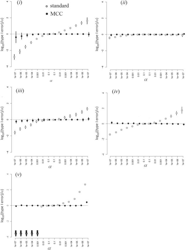
Simulations with  = 500, simulation scenarios (i)–(v). Each
  -axis is the false positive rate for a single tail of the
  distribution, with the correct threshold determined by
  permutations (values on the left are for the left tail, values on the right for the right tail). The plotted points are the actual false positive rates for these thresholds, expressed as a
  ratio compared with intended, via one-sided standard or MCC
  -values. Arrows in panel (v) show outcomes for which the logistic regression likelihood ratio statistic did not converge. Error bars represents
  SD for the 10 different simulations per scenario. Standard
  -values are often incorrect by more than 2 orders of magnitude, and substantial inaccuracy persists for
  and
and  (Figures 9 and 10 of supplementary material available at Biostatistics online).
In summary, the standard approaches often have difficulty with type I error control, if both  and
and  are skewed. However, MCC is well-behaved across all the scenarios. If the direction of skew were reversed for either
  or
or  , the conservativeness would appear on the right.
6.1. An RNA-Seq example
As a final example, incorporating several of the aspects described above, we consider the RNA-Seq expression data of Montgomery and others (2010) from  HapMap CEU cell lines, with ranked
  values from exposure to etoposide (Huang and others, 2007) used as a response
  . For these samples,
  genes which vary across the samples were used. We applied the residualization approach as described earlier, with sex as a stratified covariate. The RNA-Seq data were originally based on integer counts, which were then normalized as described in Zhou and others (2011) and covariate-residualized. We applied MCC
 to the data for all features, requiring 25 min on the desktop PC used earlier for timing comparisons.
Figure 6 (top panels) shows the results for the most significant gene as determined by MCC, although not genome-wide significant (empirical  based on
  permutations,
  ). The lower panels show an example gene that is not significant, but for which the distribution is highly multimodal, due to the presence of extreme count values in
  . Nonetheless,
  can effectively fit the density, due to its successive conditioning strategy.
Fig. 6.

Normalized RNA-Seq data vs. etoposide  . Residualized
  vs.
vs.  and null permutation histograms for the gene TEAD4 (upper panels) and AGT (lower panels). The fitted
  densities are overlaid on the histograms, and the observed
  shown as a dashed line.
7. Discussion
We have described a coherent and fast approach to perform trend testing of a single vector vs. all rows of a matrix, which is a canonical testing problem arising in genomics and other high-throughput applications. As implemented in the mcc R package, the investigator need only provide  and
and  , and possibly strata, and
  and
and  will be automatically computed.
We emphasize that the idea of approximating permutation distributions is not new. In addition to saddlepoint approaches as described (Robinson, 1982; Booth and Butler, 1990), approaches using moment approximations for density fits include (Zhou and others, 2009; Zhou and others, 2013). However, these approaches have not fully exploited the simplicity of the score statistic and the attendant extreme speed of computation achieved here. We also note that our  -values are not adjusted for multiple comparisons, and thus are most immediately useful for methods such as Bonferroni or false discovery control. However, another important aspect of our approach is that, by ensuring greater uniformity of null
  -values, each tested feature is placed on the same scale. Thus, as the computation for MCC is of the same order as computing the statistic
  itself, MCC might be subjected to family-wise (across all features) permutation, or importance sampling (Kimmel and Shamir, 2006).
Our approach largely eliminates the need to be concerned over the appropriate choice of trend statistic, or whether parametric testing can be justified for the data at hand. In specific settings, such as genotype association testing, concern over the minor allele frequencies often leads investigators to perform exact testing for a subset of markers. We clarify here that the primary difficulty arises when both  and
and  are skewed, but the effects of the fourth moments may also be noticeable for extreme testing thresholds. For standard case–control studies with samples accrued in a 1:1 ratio, skewness may not be severe. However, for the analysis of binary secondary traits, the case:control ratio may depart from 1:1, and thus
  may be highly skewed. In addition, the expense of sequence-based genotyping has increased interest in using shared or common sets of controls, which could then be much larger than the number of cases.
A possible alternative approach is to simply transform  and/or
  (e.g. to match quantiles of a normal density) so that standard approximations fit well. Although this approach may provide correct type I error, it may also distort the interpretability of a meaningful trait or phenotype. In addition, for discrete data, such as those used in case–control genetic association studies, no such transformation may be feasible. We also note that it is rare for such transformations to be considered prior to fitting GLMs, and thus our methodology remains highly relevant.
We note that the standard density approximation is intended for unconditional inference, i.e. not conditioning on the observed  and
and  . Thus, it might be considered in some sense unfair to expect a close correspondence to the permutation distribution, which is inherently conditional on the data. However, the results in Figures 5, 9, and 10 of supplementary material available at Biostatistics online are highly consistent across independent simulations, showing that if the densities of
  and
and  are skewed, standard parametric
  -values tend to be inaccurate on average. Thus, we can recommend MCC as generally preferred over standard trend testing for high-throughput datasets.
Supplementary material
Supplementary material is available at http://biostatistics.oxfordjournals.org.
Funding
This work was supported in part by the Gillings Statistical Genomics Innovation Lab, EPA RD83382501, NCI P01CA142538, NIEHS P30ES010126, P42ES005948, HL068890, MH101819 and DMS-1127914.
Supplementary Material
Acknowledgments
We thank Dr Alan Agresti for pointing out the relevance of the Hauk and Donner 1977 paper described in Appendix (see supplementary material available at Biostatistics online). We gratefully acknowledge the CF patients, the Cystic Fibrosis Foundation, the UNC Genetic Modifier Study, and the Canadian Consortium for Cystic Fibrosis Genetic Studies, funded in part by Cystic Fibrosis Canada and by Genome Canada through the Ontario Genomics Institute per research agreement 2004-OGI-3-05, with the Ontario Research Fund-Research Excellence Program. Conflict of Interest: None declared.
References
- Breslow N. E., Day N. E. (1980). Statistical methods in cancer research. Vol. 1. The analysis of case-control studies. IARC Scientific Publications 1, 5–338. [PubMed] [Google Scholar]
- Booth J. G., Butler R. W. (1990). Randomization distributions and saddlepoint approximations in generalized linear models. Biometrika 774, 787–796. [Google Scholar]
- Corcoran C., Mehta C., Patel N., Senchaudhuri P. (2001). Computational tools for exact conditional logistic regression. Statistics in Medicine 20(17–18), 2723–2739. [DOI] [PubMed] [Google Scholar]
- Cox D. R., Snell E. J. (1989). Analysis of Binary Data. Boca Raton: Chapman and Hall. [Google Scholar]
- Frisch R., Waugh F. V. (1933). Partial time regressions as compared with individual trends. Econometrica 1, 387–401. [Google Scholar]
- Good P. I. (2005). Permutation, Parametric, and Bootstrap Tests of Hypotheses. Berlin: Springer. [Google Scholar]
- Huang S. T., Duan S., Bleibel W. K., Kistner E. O., Zhang W., Clark T. A., Chen T. X., Schweitzer A. C., Blume J. E., Cox N. J. and others (2007). A genome-wide approach to identify genetic variants that contribute to etoposide-induced cytotoxicity. Proceedings of the National Academy of Sciences 10423, 9758–9763. [DOI] [PMC free article] [PubMed] [Google Scholar]
- Kennedy P. E., Cade B. S. (1996). Randomization tests for multiple regression. Communications in Statistics—Simulation and Computation 254, 923–936. [Google Scholar]
- Kimmel, Gad, Shamir Ron. (2006). A fast method for computing high-significance disease association in large population-based studies. The American Journal of Human Genetics 793, 481–492. [DOI] [PMC free article] [PubMed] [Google Scholar]
- Kulinskaya E. (2008). On two-sided P-values for nonsymmetric distributions. Arxiv (arXiv:0810:2124).
- Lehmann E. L. (1975). Nonparametrics: Statistical Methods Based on Ranks. San Francisco: Holden-Day. [Google Scholar]
- Lehmann E. L., Romano J. P. (2005). Testing Statistical Hypotheses. Berlin: Springer. [Google Scholar]
- Li Y., Willer C. J., Ding J., Scheet P., Abecasis G. R. (2010). MaCH: using sequence and genotype data to estimate haplotypes and unobserved genotypes. American Journal of Human Genetics 348, 816–834. [DOI] [PMC free article] [PubMed] [Google Scholar]
- Miller L. D., Smeds J., George J., Vega V. B., Vergara L., Ploner A., Pawitan Y., Hall P., Klaar S., Liu E. T. and others (2005). An expression signature for p53 status in human breast cancer predicts mutation status, transcriptional effects, and patient survival. Proceedings of the National Academy of Sciences 10238, 13550–13555. [DOI] [PMC free article] [PubMed] [Google Scholar]
- Montgomery S. B., Sammeth M., Gutierrez-Arcelus M., Lach R. P., Ingle C., Nisbett J., Guigo R., Dermitzakis E. T. (2010). Transcriptome genetics using second generation sequencing in a Caucasian population. Nature 4647289, 773–777. [DOI] [PMC free article] [PubMed] [Google Scholar]
- Mukherjee S., Simon J., Bayuga S., Ludwig E., Yoo S., Orlow I., Viale A., Offit K., Kurtz R., Olson S. H. and others (2011). Including additional controls from public databases improves the power of a genome-wide association study. Human Heredity 721, 21–34. [DOI] [PMC free article] [PubMed] [Google Scholar]
- Pitman E. J. G. (1937). Significance tests which may be applied to samples from any populations. II. The correlation coefficient test. Supplement to the Journal of the Royal Statistical Society 4, 225–232. [Google Scholar]
- Purcell S., Neale B., Todd-Brown K., Thomas L., Ferreira M. A., Bender J. D., Maller S. P., de Bakker P. I., Daly M. J., Sham P. C. (2007). PLINK: a tool set for whole-genome association and population-based linkage analyses. American Journal of Human Genetics 813, 559–575. [DOI] [PMC free article] [PubMed] [Google Scholar]
- Robinson J. (1982). Saddlepoint approximations for permutation tests and confidence intervals. Journal of the Royal Statistical Society 441, 91–101. [Google Scholar]
- Stokes D. C. S. M. E., Koch G. G. (2000) Categorical Data Analysis Using the SAS System. SAS Institute Inc. [Google Scholar]
- Takei N., Miyashita A., Tsukie T., Arai H., Asada T., Imagawa M., Shoji M., Higuchi S., Urakami K., Kimura H. and others (2009). Genetic association study on in and around the APOE in late-onset Alzheimer disease in Japanese. Genomics 935, 441–448. [DOI] [PubMed] [Google Scholar]
- Wright F., Strug L. J., Doshi V. K., Commander C. W., Blackman S. M., Sun L., Berthiaume Y., Cutler D., Cojocaru A., Collaco J. M. and others (2011). Genome-wide association and linkage identify modifier loci of lung disease severity in cystic fibrosis at 11p13 and 20q13. 2. Nature Genetics 436, 539–546. [DOI] [PMC free article] [PubMed] [Google Scholar]
- Zhou Y.-H., Mayhew G., Sun Z., Xu X., Zou F., Wright F. A. (2013). Space-time clustering and the permutation moments of quadratic forms. Statistics 21, 292–302. [DOI] [PMC free article] [PubMed] [Google Scholar]
- Zhou C., Wang H. J., Wang Y. M. (2009). Efficient moments-based permutation tests. Advances in Neural Information Processing Systems, pp. 2277–2285. [PMC free article] [PubMed] [Google Scholar]
- Zhou Y. H., Xia K., Wright F. A. (2011). A powerful and flexible approach to the analysis of RNA sequence count data. Bioinformatics 2719, 2672–2678. [DOI] [PMC free article] [PubMed] [Google Scholar]
Associated Data
This section collects any data citations, data availability statements, or supplementary materials included in this article.