Using in vivo imaging to measure RNA mobility in Xenopus laevis oocytes

Abstract

RNA localization in the Xenopus oocyte is responsible for the establishment of polarity during oogenesis as well as the specification of germ layers during embryogenesis. However, the inability to monitor mRNA localization in live vertebrate oocytes has posed a major barrier to understanding the mechanisms driving directional transport. Here we describe a method for imaging MS2 tagged RNA in live Xenopus oocytes to study the dynamics of RNA localization. We also focus on methods for implementing and analyzing FRAP data. This protocol is optimized for imaging of the RNAs in stage II oocytes but it can be adapted to study dynamics of other molecules during oogenesis. Using this approach, mobility can be measured in different regions of the oocyte, enabling the direct observation of molecular dynamics throughout the oocyte.

1. Introduction

Active transport of mRNA via the cytoskeleton is a widely used mechanism for generating and maintaining asymmetric distribution of cellular determinants across a continuous cytoplasm in both somatic and germ cells. Xenopus oocytes are an important model system for studying RNA localization and vertebrate development. In Xenopus laevis, oogenesis occurs over a period of four to eight months [1] during which an oocyte progresses through six stages of growth and development. Localization of maternal RNAs occurs during the early stages (I-III) of oogenesis, and the cell maintains the localization of these RNAs throughout the entire process of oocyte maturation. During stages II-III of oogenesis, mRNAs such as Vg1 and VegT, termed the “late pathway” RNAs, are localized via the microtubule cytoskeleton through the vegetal cytoplasm to their ultimate destination at the vegetal cortex where they remain anchored for the remainder of oogenesis (reviewed in [2]). This localization event is responsible for the establishment of the developmental axes as well as subsequent identity of the germ layers in embryogenesis [2].

Previously, imaging experiments in Xenopus oocytes have been predominately performed using fixed cells. Imaging fixed oocytes is facilitated by the use of a clearing agent that renders the yolk optically clear but precludes the use of fluorescent proteins [3]. While these techniques have provided snapshots that inform our understanding of late pathway mRNA localization, they are unable to address questions about the dynamics of transport and how actively localizing mRNA is maintained in its stage-specific localization pattern despite the long time periods required to progress through the stages of oogenesis. Live cell imaging using fluorescent proteins offers a powerful approach to answer both qualitative and quantitative questions about the dynamics and kinetics of RNA localization in the early stages of Xenopus oogenesis.

To study the process of RNA localization in live Xenopus oocytes we adapted the MS2 system for labeling RNAs in vivo [4]. Briefly, we created a transcript that contains both the MS2 bacteriophage stem loops and the vegetal localization element (VLE) of the Vg1 mRNA (VLE-MS2) [5]. The VLE is sufficient to direct RNA to localize vegetally via the late pathway [6]. MS2 stem loops bind tightly to the MS2 coat protein (MCP), which has been fused to the red fluorescent protein mCherry (MCP mCherry). The VLE directs the exogenous RNA to localize while the MS2 stem loops bind the MCP mCherry, creating a mCherry tag on the reporter RNA. This creates a system in which a late pathway localizing RNA can be imaged in live cells, enabling the study of the dynamic aspects of RNA localization.

The large size of the Xenopus oocyte allows facile microinjection of exogenous RNAs as well as significant amounts of material for biochemical and other in vitro approaches, but it also presents challenges for in vivo imaging. First, the large, spherical size of the oocytes interferes with the ability to image whole oocytes at high magnification. Second, Xenopus oocytes have strong autofluorescence throughout the vegetal cytoplasm when imaged with a 488nm laser line. This property significantly impairs the use of any green or yellow fluorescent proteins or fluorophores. Additionally, any live cell imaging of oocytes must be done using early stage oocytes before yolk production renders the oocyte opaque. Two-photon microscopy can extend this slightly, but the opacity of late stage oocytes remains a barrier to performing live cell microscopy.

The MS2 system of in vivo RNA labeling provides a means to study the dynamics of RNA localization in living Xenopus oocytes. We previously used this method to identify two distinct regions of the vegetal cytoplasm that the RNA transits through, one of which is dynein directed and another which utilizes both dynein and kinesin motors. In the latter region we observed bidirectional movement of RNA through the use of in vivo imaging of VLE-MS2 RNA[5]. This method can be readily adapted to any live cell imaging analysis including fluorescence recovery after photobleaching (FRAP), photoactivation, and photoconversion. Here we describe the approach used by our laboratory for the preparation of Xenopus oocytes for in vivo imaging of RNA motility as well as the analysis of FRAP data from cortically localized RNA.

2. Methods

1.1 Oocyte acquisition

Oocytes are isolated from mature Xenopus laevis females. Albino frogs are used to eliminate any possibility of pigment obscuring the imaging. The ovary is surgically removed from the frog and placed in 1x MBSH buffer [88mM NaCl, 1mM KCl, 2.4M NaHCO₃, 0.82mM MgSO₄*7H₂O, 0.33mM Ca(NO₃)*4 H₂O, 0.41 mM CaCl*6H2O), 10mM HEPES (pH 7.6)]. Dissecting scissors are used to finely cut the ovary into small sections. These pieces are defolliculated in a collagenase solution [3 mg/mL collagenase (Sigma-Aldrich C0130), 0.1M K₂HPO 4 (pH 7.4)] by shaking vigorously at room temperature until oocytes are separated from each other. This usually takes between 10-15 minutes. Take care not to over incubate the oocytes in the collagenase solution as it may cause them to disintegrate. Allow the oocytes to settle in the collagenase solution for 5 minutes before aspirating off most of the solution, making sure to avoid removing the smaller oocytes which will settle on top. Wash oocytes in 1×MBSH, repeating the 5 minute wait and aspiration between washes until the wash liquid is clear.

To separate the oocytes into stages, they are passed through meshes of various pore sizes. First, the large, older (Stages IV-VI) oocytes are separated from the small, younger (Stages I-III) oocytes by passing all of the oocytes through a 700μm mesh. Oocytes are collected directly into a dish containing MBSH. The mesh should be immersed in the MBSH before the oocytes are passed through. The stage I-III oocytes are further fine sorted by passing through smaller meshes. A 475μm mesh will allow stage I-II oocytes to pass through and retain stage III and early IV oocytes. A 300μm mesh is then used to separate out stage I/early II from late stage II/early stage III oocytes. This facilitates the subsequent hand sorting of oocytes for microinjection. All meshes are Sefar Nitex nylon meshes of the specified size. Once the oocytes are sorted, they can be counted and selected using a stereomicroscope.

For FRAP studies, it is critically important that the oocytes not be opaque. As oocytes progress through stage II, opacity increases which impedes light transmission through the oocyte, making FRAP studies anywhere other than at the cortex highly challenging (Figure 1). Stage I oocytes are transparent and ideal for live imaging studies. Previous work on the localization of the early pathway mRNAs nanos1 (Xcat2) and Xdazl, used FRAP of fluorescently injected RNAs in stage I oocytes to show that early pathway RNAs localize to the mitochondrial cloud by a diffusion/entrapment mechanism as opposed to the active transport mechanism used by late pathway RNAs [7]. However, late pathway RNAs are not localized in stage I oocytes, so they are not suited for studying their localization. We use early stage II oocytes to image late pathway RNA localization, as they are both competent to localize an exogenous reporter RNA containing the VLE and are still translucent enough to allow in vivo imaging.

Figure 1.

Opacity of Xenopus laevis oocytes as they progress from early stage II to late stage II. Early stage II oocytes (left) are ideally suited for imaging. As oogenesis progresses (left to right) it becomes increasingly difficult to image internal regions of the cytoplasm. Scale bar is 100μm.

1.2 Microinjection and oocyte selection

Appropriate expression levels of MCP mCherry protein are obtained by microinjecting stage II oocytes with 2nl of 250nM MCP mCherry RNA in MBSH solution, followed by overnight culture in OCM [50% L-15 media, 15mM HEPES (pH 7.6), 2μg/mL insulin, with 10μl/mL penicillin/streptomycin, 10μl/mL Gentamycin, 5μl/mL Nystatin] at 18°C to allow for expression of the protein. The next day the oocytes are viewed on a stereomicroscope equipped with fluorescence lighting (e.g., Zeiss Lumar V12 fluorescence stereomicroscope) and imaged using a Cy3/TRITC filter. Cells expressing mCherry are selected and subsequently microinjected with either 2nl 250nM MS2-VLE RNA or 2nl of 250nM MS2-βglobin RNA, a non-localizing control RNA (Figure 2A) [5]. Oocytes are cultured in OCM until they are ready to be imaged. They can be imaged as early as two hours after injection but 8-18 hours is usually preferred. An additional sorting step on a fluorescence stereomicroscope can be useful to select for cells that show a brightly fluorescent signal on the vegetal cortex before mounting for in vivo imaging. The sorting steps ensure that all the cells to be embedded and subsequently imaged contain both MCP mCherry protein and the reporter MS2 tagged RNA that has been properly localized (Figure 2B). Note: If imaging at early time points (e.g. 2 hours) the accumulation of RNA at the vegetal cortex will not be visible, and the vegetal cytoplasm will need to be identified without the aid of fluorescence accumulation. The autofluorescence seen when exciting with the 488 laser line can aid in identification of the vegetal cytoplasm if looking at cells shortly after injection of the RNA or in control cell injected with a non-localizing βglobin control RNA.

Figure 2.

A) Schematic of the vegetal localizing VLE-MS2 RNA and the non-localizing control RNA, βglobin-MS2. Each element is fused with 24 tandem MS2 stem loops. These stem loops bind the MS2 coat protein with a C-terminal mCherry protein tag (MCP mCh).

B) Procedure for the preparation of oocytes for live cell imaging. The top panel is a schematic while the bottom panel shows representative images of each step. Early stage II oocytes are sorted and microinjected with MCP mCherry RNA, which is allowed to express overnight. Oocytes showing appropriate levels of mCherry expression are manually sorted on a fluorescence dissecting microscope. These oocytes are given a second injection with RNA fused to 24 tandem MS2 repeats and cultured to localize overnight. Oocytes that show accumulation of fluorescent RNA at the vegetal pole of the oocyte are selected for imaging. In all images the vegetal pole is at the bottom. Red arrowhead indicates the GV while the green arrowhead indicates the vegetal cytoplasm. Scale bar is 100μm.

2.3 Oocyte mounting for imaging

Maintaining a constant position over time is critical for the acquisition of FRAP data. Oocytes in liquid culture are susceptible to small movements which affects the ability to collect data over the time period required to complete a FRAP experiment. To immobilize the oocytes during the imaging they are placed in 35mm fluorodishes (WPI Inc, FD35-100) in OCM containing 1% low melting temperature agarose. For imaging, the OCM should be made with L-15 that does not contain phenol red. The solution should then be kept warm in a 37°C water bath to prevent it from solidifying prematurely, but not above 37°C to prevent any heat damage to the oocytes. To expedite this process a 2% agarose in 2x OCM stock is made. This allows for a 1:1 combination of oocytes in OCM to immobilizing media. The following steps need to be performed as quickly as possible in order to allow the oocytes to be manipulated into the correct orientation for imaging before the agar has solidified. It is highly recommended to have everything set up in close proximity to a stereomicroscope to expedite the embedding process. First, add oocytes in OCM to the fluorodish using a Pasteur pipet. Initially try to add between 5-10 oocytes per dish. This number may be increased slightly with familiarity of the orientation process. Then add an equal volume of the 2% agarose in 2x OCM immobilization media to the fluorodish. Next, oocytes must be oriented with their vegetal poles facing towards the bottom of the fluorodish, which will allow for imaging through the vegetal half of the oocyte. However, it is generally preferred for the pole to be at an angle offset (~15-35°C is ideal) from the bottom of the plate (Figure 3A). This allows for a cross section that transverses the vegetal cytoplasm in a single image without prohibitive signal attenuation that is an effect of moving too far up from the objective in the z-axis (Figure 3B). This orientation must be done using tools for micromanipulation of the oocytes on a low magnification stereomicroscope. To do this with minimal stress to the oocytes, attach a short hair (e.g. eyelash) to the end of a Pasteur pipet sealed with glue or wax. This allows gentle manipulation of the oocyte into the correct position for imaging while the immobilization media is solidifying (2-3 minutes).

Figure 3.

A) Oocytes are oriented in fluorodishes with the vegetal poles facing down and at an angle, for use with inverted confocal microscopes.B) The poles are offset in the dish at an angle that allows for the cells to be imaged through the entire vegetal cytoplasm.

2.4 Image Acquisition

Imaging should be performed on a confocal or two-photon microscope equipped with appropriate laser lines for both imaging and photobleaching. Photobleaching is ideally performed at 100% laser power for the fluorophore being imaged. However, since mCherry has a longer emission wavelength than green or yellow fluorophores it may be necessary to bleach using a 405 laser. Care should be taken to use conditions that will bleach your fluorophore of interest but not more than necessary in order to minimize the production of reactive oxygen species, which can cause cellular damage and stress responses.

FRAP data requires the definition of regions of interest (ROI). The size and shape of the ROI should be determined based on the individual requirements of the experiment. The ROI of experimental interest is photobleached but additionally there are two control ROIs that are necessary for adjustment and normalization of the FRAP data. These ROIs must be the same size as the experimental ROIs. First, fluorescence data ROI_o(t) is collected outside of the sample and this is used to correct for the black level of the imaging field. Additionally, data ROI_n(t) must be collected from within the sample and does not get bleached. The changes in the fluorescence in this area are used to correct for photobleaching throughout the length of the experiment.

2.5 Image Analysis

The raw time series fluorescence data for each ROI in the vegetal cytoplasm is then corrected and normalized. To correct for acquisition photobleaching, the adjusted fluorescence time series A(t) is calculated as

$$A(t)=F(t)\times \frac{F_{\mathrm{pre}}}{F_{\mathrm{n}}(t)}=(\mathrm{ROI(}t)-{\mathrm{ROI}}_o\text{(}t))\times \frac{({\mathrm{ROI}}_n(1)-{\mathrm{ROI}}_o(1))}{({\mathrm{ROI}}_n(t)-{\mathrm{ROI}}_o(t))},$$ (1)

where F(t) is the background subtracted fluorescence at time t, F_pre is the background subtracted average intensity for all the prebleach frames and F_n(t) is the background subtracted fluorescence intensity value of a neighboring region at time t. Here ROI(t) corresponds to the raw fluorescence data from the photobleached cortical region of interest at time t, and ROI_o(t) and ROI_n(t) are fluorescence data from the non-photobleached regions outside and inside the oocyte respectively at time t. The second equality in equation (1) shows that F(t) corresponds to subtracting the background fluorescence ROI_o(t) from the fluorescence intensity of interest ROI(t), F_pre corresponds to subtracting the background fluorescence of the prebleach frames ROI_o(1) from prebleach fluorescence outside the cortical region ROI_n(1), and F_n(t) is the difference of the background fluorescence intensity ROI_o(t) from the fluorescence at the neighboring region outside the cortical region ROI_n(t).

The adjusted fluorescence data A(t) can be further normalized against prebleach values, yielding normalized adjusted fluorescence time series A_norm (t):

$$A_{\mathrm{norm}}(t)=\frac{A(t)}{f_{\mathrm{pre}}}=\frac{A(t)}{(\mathrm{ROI}(1)-({\mathrm{ROI}}_o(1))},$$ (2)

where f_pre is the background subtracted average prebleach intensity in the cortical region ROI. As in the case of adjusted data A(t), we do not calculate the normalized fluorescence in the regions outside the sample (o) and inside the sample (n) since these areas are not photobleached, so that the mobility of mRNA in these regions cannot be determined.

Either of the resulting time series data A(t) or A_norm(t) can be analyzed to extract binding and diffusion information from FRAP experiments. Other studies have provided a third normalization technique that can be applied to adjusted, normalized fluorescence data A_norm(t) to yield the time series N(t). This method requires that the intensity values are further normalized so that the fluorescence intensity right after the bleach is set to 0, and the one at the plateau level is set to 1 [8]. The equation for this normalized time series data N(t) is:

$$N(t)=\frac{A_{\mathrm{norm}}(t)-A_{\mathrm{norm}}(1)}{A_{\mathrm{norm},\mathrm{pl}}-A_{\mathrm{norm}}(1)},$$ (3)

where A_norm(1) is the photobleach corrected fluorescence intensity at the first time point after bleaching and A_norm,pl is the average photobleach corrected fluorescence intensity at the plateau. In practice, A_norm,pl can be calculated as the average of the last 10% values of photobleach corrected fluorescence intensity A_norm measured in the experiment. We use A(t) and N(t) in our subsequent analysis of the FRAP fluorescence intensity curves (Figure 4).

Figure 4.

Fluorescence intensity normalizations for FRAP recovery curves. Adjusted fluorescence data (left, A(t)) is corrected for acquisition photobleaching, normalized adjusted fluorescence data (center, A_norm(t)) is further normalized against prebleach values, and normalized data (right, N(t)) has its values set to 0 right after the bleach and 1 at the plateau value.

Assuming that there is no active transport of VLE RNA in the cortical RNA population, the adjusted or normalized FRAP fluorescence intensity curves are fit to an established model [9]. The equations for the single binding protein reaction involve a population of free molecules that can diffuse, as well as a population of bound complexes. The two populations interact via binding and dissociation with rates k_on and k_off. The main assumptions for the approach in this model are that the RNA population achieves equilibrium before photobleaching, and that the binding sites are part of a large, immobile complex.

Previous FRAP experiments in this system assume that mRNA diffusion across the bleach spot is fast compared to the timescale of binding of mRNA to sites it interacts with [5] [7]. Under this assumption, the fluorescence intensity recovery is called interaction-limited as described in Rino et al, 2014 or, equivalently, it satisfies the dominant simplification of the model in Sprague et al, 2004 [9] [10]. This assumption means that the adjusted and the normalized fluorescence curves can be fit to the exponential model:

$$\mathrm{frap}(t)=a\left(1-\frac{k_{\mathrm{on}}}{k_{\mathrm{on}}+k_{\mathrm{off}}}{e}^{-k_{{\mathrm{off}}^t}}\right),$$ (4)

or equivalently to the formulation

$$\mathrm{frap}(t)=a-c{e}^{-k_{{\mathrm{off}}^t}},$$ (5)

where $c=a\frac{k_{\mathrm{on}}}{k_{\mathrm{on}}+k_{\mathrm{off}}}$ and frap(t) = A(t) or N(t).

Half times of recovery t_1/2 based on the above model can be calculated using the equation:

$$t_{1/2}=\frac{\ln (2)}{k_{\mathrm{off}}}.$$ (6)

The advantage of using equation (5) instead of equation (4) is that fits of adjusted data frap(t) = A(t) and of normalized data frap(t) = N(t) give similar results for k_off and thus for halftimes t_1/2.

We analyzed the data from the three ROIs for the cortical RNA using the above methodology. Using this method and fitting with the least squares norm, both the adjusted and normalized data sets show very similar halftimes t_1/2. Estimates of the rates k_on and k_off can also be calculated by fitting fluorescence intensity curves to equation (4). Cortical RNA has been hypothesized to be a highly stable complex as the RNA remains localized from stage II through the end of oogenesis [11]. The FRAP results discussed here confirm that the cortical fraction of RNA is present in a highly stable complex (Figure 5).

Figure 5.

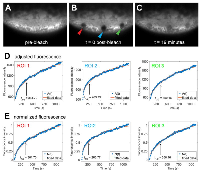
A-C) Images are shown of a representative oocyte in which three 5μm circular areas of cortical VLE-MS2 RNA bound by MCP mCherry were bleached with four iterations of the 405 laser at 100% power. Fluorescence recovery was monitored for 19 minutes post-bleach. A) Vegetal cortical cytoplasm is shown before bleaching (pre-bleach). B) Arrowheads indicate the experimental regions bleached: ROI 1 (red), ROI 2 (blue) and ROI 3 (green). C) The vegetal cortical cytoplasm is shown in the same oocyte 19 minutes after bleaching. D-E) Adjusted fluorescence intensity curves (D) and normalized fluorescence intensity curves (E) were fitted with equation (5). The black vertical lines indicate the halftime of recovery for each fluorescence curve.

The Matlab routine fit was used to fit the model equation (5) to experimental data (The MathWorks, Natick, MA). In order to optimize the fluorescence data fits and ensure convergence to reasonable parameter values, we can specify initial guesses for the parameters a, k_off and c in equation (5) as well as bounds for these parameters. Given the meaning of a and c, we search for positive parameters that are bounded from above by a value larger than the maximum fluorescence data (in practice, this can be set to 2 * max (frap(t))) and choose the last fluorescence data point in the FRAP recovery as the initial guess for these parameters in the Matlab fit command. The parameter k_off is most relevant in estimating halftimes and mobility: we search for a positive parameter, relax the upper bound to infinity, and choose 0 as the initial guess in the Matlab fit command to optimize the data fitting.

3. Concluding Remarks

We have described a method for the imaging and analysis of RNA in live Xenopus oocytes. This system has a unique set of challenges but offers a significant opportunity for study of a complex pathway of RNA localization during development. For example, the large size of the oocyte facilitates the acquisition of multiple FRAP ROIs in different regions of the same cell. This allows for the simultaneous analysis of motility in regions of the cell that are carrying out distinct steps in the transport pathway. The preparation and selection of oocytes at each stage is critical for the optimization of imaging time. While this article focuses on FRAP, the techniques described above are widely applicable to any live cell imaging in Xenopus oocytes and can be adapted for use with photoconversion or photoactivation, as we have shown previously [5]. Additionally, development of analogous methods of tagging RNAs (e.g. PP7 hairpins bound by the PP7 coat protein (PCP)) to study RNA mobility in vivo can be used in place of, or in concert with the MS2 system [12]. Using two different labels, this method can be easily adapted to monitor the kinetics of two different RNA populations within the same cell.

We also describe a method for analysis of FRAP data in ooctyes that produces similar rates of k_off and thus halftimes of RNA recovery for different data normalizations and different regions of interest. The halftime and binding/unbinding rate estimates obtained from fitting corrected FRAP data are useful in that they may provide a comparison of mobility of RNA in wild-type oocytes with RNA mobility in oocytes where motor protein function has been disrupted. As noted above, this FRAP analysis approach assumes that there is no active transport of RNA [7]. This is a reasonable assumption for cortical regions of the Xenopus oocyte as shown in Figure 5. However, it is known that RNA localization in the vegetal cytoplasm area depends on the bidirectional transport of RNA by molecular motor proteins kinesin and dynein [5] [13]. Including movement of RNA in analyzing FRAP fluorescence intensity curves would require extending the existing differential equations [9] to account for populations of RNA that are actively transported in the cell. In that case, fitting to the simplified equation (5) would need to be replaced by a more carefully devised parameter fitting technique.

Highlights.

• We describe a method for the preparation, imaging, and analysis of Xenopus oocytes for FRAP studies

• Stage II oocytes were injected with MCP mCherry RNA for expression and MS2 VLE RNA for tracking vegetal RNA localization

• The RNA mobility at the cortex was analyzed by FRAP

• FRAP analysis equations are used to model different FRAP data normalizations.

References

- 1.Dumont JN. J Morphol. 1972;136:153–179. doi: 10.1002/jmor.1051360203. [DOI] [PubMed] [Google Scholar]
- 2.Medioni C, Mowry K, Besse F. Development. 2012;139:3263–3276. doi: 10.1242/dev.078626. [DOI] [PMC free article] [PubMed] [Google Scholar]
- 3.Gagnon JA, Mowry KL. Methods Mol Biol. 2011;714:71–82. doi: 10.1007/978-1-61779-005-8_5. [DOI] [PMC free article] [PubMed] [Google Scholar]
- 4.Bertrand E, Chartrand P, Schaefer M, Shenoy SM, Singer RH, Long RM. Mol Cell. 1998;2:437–445. doi: 10.1016/s1097-2765(00)80143-4. [DOI] [PubMed] [Google Scholar]
- 5.Gagnon JA, Kreiling JA, Powrie EA, Wood TR, Mowry KL. PLoS Biology. 2013;11:e1001551. doi: 10.1371/journal.pbio.1001551. [DOI] [PMC free article] [PubMed] [Google Scholar]
- 6.Mowry KL, Melton DA. Science. 1992;255:991–994. doi: 10.1126/science.1546297. [DOI] [PubMed] [Google Scholar]
- 7.Chang P, Torres J, Lewis RA, Mowry KL, Houliston E, King ML. Mol Biol Cell. 2004;15:4669–4681. doi: 10.1091/mbc.E04-03-0265. [DOI] [PMC free article] [PubMed] [Google Scholar]
- 8.Axelrod D, Koppel DE, Schlessinger J, Elson E, Webb WW. Biophys J. 1976;16:1055–1069. doi: 10.1016/S0006-3495(76)85755-4. [DOI] [PMC free article] [PubMed] [Google Scholar]
- 9.Sprague BL, Pego RL, Stavreva DA, McNally JG. Biophys J. 2004;86:3473–3495. doi: 10.1529/biophysj.103.026765. [DOI] [PMC free article] [PubMed] [Google Scholar]
- 10.Rino J, Martin RM, Carvalho T, Carmo-Fonseca M. Methods. 2014;65:359–366. doi: 10.1016/j.ymeth.2013.08.010. [DOI] [PubMed] [Google Scholar]
- 11.Gagnon JA, Mowry KL. Crit Rev Biochem Mol Biol. 2011;46:229–239. doi: 10.3109/10409238.2011.572861. [DOI] [PMC free article] [PubMed] [Google Scholar]
- 12.Hocine S, Raymond P, Zenklusen D, Chao JA, Singer RH. Nat Methods. 2013;10:119–121. doi: 10.1038/nmeth.2305. [DOI] [PMC free article] [PubMed] [Google Scholar]
- 13.Messitt TJ, Gagnon JA, Kreiling JA, Pratt CA, Yoon YJ, Mowry KL. Dev Cell. 2008;15:426–436. doi: 10.1016/j.devcel.2008.06.014. [DOI] [PMC free article] [PubMed] [Google Scholar]