The temporal scaling of Caenorhabditis elegans ageing

Abstract

The process of ageing makes death increasingly likely, but involves a random aspect that produces a wide distribution of lifespan even in homogeneous populations^1,2. The study of this stochastic behaviour may link molecular mechanisms to the ageing process that determines lifespan. Here, by collecting high-precision mortality statistics from large populations, we observe that interventions as diverse as changes in diet, temperature, exposure to oxidative stress, and disruption of genes including the heat shock factor hsf-1, the hypoxia-inducible factor hif-1, and the insulin/IGF-1 pathway components daf-2, age-1, and daf-16 all alter lifespan distributions by an apparent stretching or shrinking of time. To produce such temporal scaling, each intervention must alter to the same extent throughout adult life all physiological determinants of the risk of death. Organismic ageing in Caenorhabditis elegans therefore appears to involve aspects of physiology that respond in concert to a diverse set of interventions. In this way, temporal scaling identifies a novel state variable, r(t), that governs the risk of death and whose average decay dynamics involves a single effective rate constant of ageing, k_r. Interventions that produce temporal scaling influence lifespan exclusively by altering k_r. Such interventions, when applied transiently even in early adulthood, temporarily alter k_r with an attendant transient increase or decrease in the rate of change in r and a permanent effect on remaining lifespan. The existence of an organismal ageing dynamics that is invariant across genetic and environmental contexts provides the basis for a new, quantitative framework for evaluating how and how much specific molecular processes contribute to the aspect of ageing that determines lifespan.

Body temperature is a major determinant of lifespan in poikilotherms^3–5 that also influences mammalian ageing⁶. From 20 °C to 33 °C, the mean lifespan of C. elegans decreases 40-fold⁷. To explore the impact of temperature on the actual distribution of lifespans, we used our automated imaging technology⁸ to collect highly resolved mortality data in multiple replicate populations placed across this temperature range (Methods). From these data we estimated the survival curve S(t), which is the probability of being alive at time t, and the hazard function h(t) = −d log(S(t))/dt, which is the instantaneous risk of death at time t (Supplementary Note 1.1 and Methods).

In many invertebrates, changes in temperature alter the rate at which the risk of death increases with time^4,5,9. Our lifespan data, controlled for environmental heterogeneity (see Statistical methods section in Methods), confirmed this effect. However, we further observed that changes in temperature appeared to shift h(t) by an equal and opposite amount in magnitude and time when plotted on a log–log scale, suggesting that between any two temperatures T₀ and T₁, λh_T1(t) = h_T0(λ⁻¹t) independent of any particular parametric form of h(t). This change in hazard corresponds to a simple stretching of the survival function along the time axis by a dimensionless scale factor λ: S_T1(t) = S_T0(λ⁻¹t) (Supplementary Note 1.2). The sole effect of changes in body temperature on lifespan therefore appeared to be a temporal rescaling of mortality statistics.

To confirm this effect, we applied an accelerated failure time (AFT) regression model¹⁰ in which lifespan distributions that only differed by temporal scaling would have identically distributed residuals (Supplementary Notes 1.3 and 1.4 and Methods). To identify any significant differences between AFT residual distributions, we applied a Kolmogorov–Smirnov test adapted to censored data (Supplementary Note 2). We identified no significant temperature-dependent deviations from temporal scaling within two thermal ranges: 19–30 °C and 30.5–33 °C (Fig. 1b–d and Extended Data Figs 1–3). Populations above 30.5 °C exhibited a more pronounced late-age deceleration (Fig. 1e, Extended Data Fig. 3 and Supplementary Note 1.4), consistent with an increased heterogeneity¹¹ (Supplementary Note 3). Yet, even at high temperatures, the observed hazard function appears to be dominated more by ageing (for example, a progressive increase in the hazard) than by chance events that would produce a constant hazard (that is, non-ageing).

Figure 1. Environmental determinants rescale C. elegans lifespan distributions.

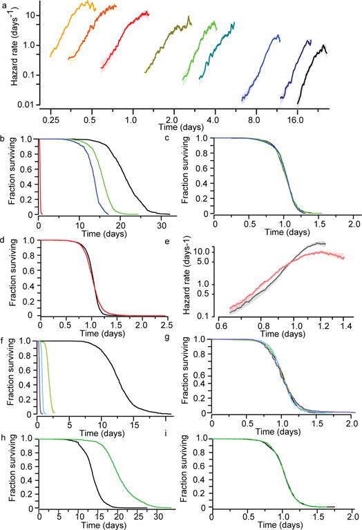
a, Populations grown at 20 °C were transferred on their second day of adulthood to a final temperature of (right to left) 20.1 °C (black), 23.7, 25.2, 29.1, 30, 30.9, 31.3, 32.5, and 32.6 (yellow). Individual lifespans were collected⁷ and used to estimate the hazard function of each population using numerical differentiation of the Kaplan–Meier survival estimator (solid lines). The shaded areas represent the 95% confidence bands of the true hazard (Statistical methods). b, The lifespan of individuals living at 20, 25, 27, and 33 °C. c, The data in b were fitted with an AFT model log(y_i) = βx_i + ε_i to remove differences in timescale (Methods and Supplementary Note 1.3). The AFT residuals exp(ε_i) corresponding to populations at 20, 25, and 27 °C are plotted using the Kaplan–Meier survival estimator. d, The AFT residuals corresponding to populations held at 25 (black) and 33 °C (red) are plotted using the Kaplan–Meier survival estimator. e, Hazard functions were estimated from the 25 and 33 °C AFT residuals. f, The survival curves of populations exposed to 0 (black), 1.5 (blue), 3 (green), and 6 mM (red) tBuOOH. g, The AFT residuals for the data of f. h, The survival curves of animals cultured on live E. coli (black) and ultraviolet-inactivated E. coli (green). i, The AFT residuals for the data of h.

We then asked whether other interventions could produce a temporal scaling. Since oxidative damage has been linked to ageing across taxa^12,13, we quantified the effect of the oxidant tert-butyl hydroperoxide (tBuOOH) and found that it quantitatively rescales lifespan distributions in a dose-dependent manner up to 3 mM (Kolmogorov–Smirnov P > 0.02) with significant deviations observed only at 6 mM (Kolmogorov–Smirnov P = 9 × 10⁻⁴; Fig. 1f–g and Extended Data Fig. 4).

To further explore the range of interventions that might yield temporal scaling, we considered three members of the insulin/IGF-1 pathway^5,9: daf-16, a transcription factor required for lifespan extension by multiple signals¹⁴, age-1, a regulatory kinase upstream of daf-16, and daf-2, the insulin/IGF receptor, all of which influence both lifespan and thermal stress resistance⁷. Each mutant population exhibited a lifespan distribution rescaled from the wild-type distribution, both at 20 °C (Kolmogorov–Smirnov P > 0.015; Fig. 2a–e) and at 33 °C (Kolmogorov–Smirnov P > 0.017; Extended Data Fig. 4). The insulin/IGF receptor daf-2 influences the activity of the heat shock factor hsf-1 (ref. 15), and disruption of hsf-1 also shortens lifespan by temporal rescaling (Kolmogorov–Smirnov P > 0.2; Fig. 2c, f). Elimination of the hypoxia-inducible transcription factor hif-1, known to influence lifespan through daf-16-dependent mechanisms¹⁶, behaved likewise (Kolmogorov–Smirnov P > 0.2; Extended Data Fig. 4).

Figure 2. Genetic determinants rescale C. elegans lifespan distributions.

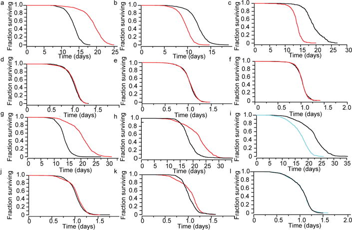
Survival curves are shown for (a) daf-2(e1368) (red) and wild type (black) at 25 °C, (b) daf-16(mu86) (red) and wild type (black) at 25 °C, and (c) hsf-1(sy441) (red) and wild type (black) at 20 °C. d–f, The AFT residuals corresponding to the data in a–c respectively. Survival curves are shown for (g) eat-2(ad1116) (red) and wild type (black) at 20 °C, (h) nuo-6(qm200) (red) and wild type (black) at 25 °C, and (i) nuo-6(qm200) populations held at 20 °C and 25 °C. j–l, The AFT residuals corresponding to the data in g–i respectively.

Since changes in nutrition alter lifespan across taxa¹⁷, we considered two modifications of C. elegans diet: ultraviolet inactivation of the bacterial food source¹⁸ and disruption of feeding behaviour by the eat-2(ad1116) mutation¹⁹. Ultraviolet inactivation of bacteria extended lifespan via temporal scaling (Kolmogorov–Smirnov P > 0.2; Fig. 1h, i). In contrast, eat-2(ad1116) populations exhibited a significant deviation from temporal scaling (Kolmogorov–Smirnov P = 5 × 10⁻⁵), with a disproportionate increase in the standard deviation of lifespan compared with the mean (Fig. 2g, j). We also noted that eat-2(ad1116) populations exhibited a substantially increased variation in developmental timing. While such variation does not affect lifespan statistics based on manually synchronized young adults (Methods), it is possible that the causes of this developmental variation also underlie the increased variation of lifespan. We found that disruption of the mitochondrial complex I in nuo-6(qm200) populations produced analogous effects on developmental timing with a deviation from temporal scaling of lifespan similar to eat-2(ad1116) (Kolmogorov–Smirnov P > 3 × 10⁻¹⁸; Fig. 2h, k). Yet, populations with either allele exhibited temporally rescaled lifespan distributions in response to temperature changes (Kolmogorov–Smirnov P > 0.2; Fig. 2i, l and Extended Data Fig. 4). We conclude that while eat-2(ad1116), nuo-6(qm200), and shifts in temperatures from below to above 30 °C alter lifespan distributions outside the temporal scaling model, these interventions do not eliminate the ability of C. elegans to respond to subsequent interventions with temporal scaling. Temporal scaling thus appears to be a pervasive response to interventions of diverse modality and intensity.

A temporal scaling would arise if all physiological determinants of the risk of death in C. elegans acted as if they were jointly governed by a single stochastic process whose rate constant alone was altered by interventions (Supplementary Note 4). If the risk of death was determined in this way, we reasoned that transient interventions early in adulthood would produce a persistent temporal shift, not a scaling, of mortality statistics (Supplementary Note 4.3). To test this, we focused on temperature, which can be quantitatively, rapidly, and reversibly switched at any age from a baseline temperature T₀ to a transient temperature T₁ (Fig. 3a). We confirmed that transient exposure to higher temperatures produced a permanent shortening of lifespan⁵ (Fig. 3b). We found that this shortening consisted of a temporal shift of the lifespan distribution (Fig. 3c, d) S_T1(t) = S_T0(t − Δ_τ) that matches the magnitude of shift Δ_τ predicted if time were rescaled only for the period τ that animals were held at the transient temperature: Δ_τ = τ (1 – λ⁻¹), with λ the scale factor relating populations always held at T₁ to populations always held at T₀ (Fig. 3e, f, Supplementary Note 4.3, Supplementary Table 2 and Extended Data Fig. 5). In a complementary experiment, we found that exposure to high temperature for different periods τ also gave shifts with the predicted magnitude (Extended Data Fig. 5). It appears, therefore, that the temporal scaling observed in Fig. 1a and the temporal shifting of Fig. 3 are compatible with a single model in which interventions alter the effective rate constant of a stochastic process governing those aspects of C. elegans physiology that determine risk of death. This process is evidently ongoing even very early in adulthood and is governed by the same rate constant as in late adulthood.

Figure 3. Transient interventions during early adulthood shift the lifespan distribution.

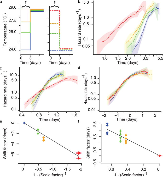
a, A schematic: populations were placed at 24 °C (blue), 26 °C (green), 27.5 °C (orange), and 29 °C (red). After τ = 3.2 days, sub-populations were transferred to either 24 °C or 29 °C for the remainder of their lives. b, The hazard rate was estimated using the remaining lifespan of populations transferred to the final temperature of 29 °C. c, To test for temporal scaling between the populations shown in b, death times were fitted with the regression model log(y_i) = βx_i + ε_i, in which exp(β_i) is the best estimate for the scale factor λ. The residuals exp(ε_i) are plotted as hazard functions in the colour scheme of a. d, To test for temporal shifts between the populations shown in b, death times were fitted with the regression model y_i = βx_i + ε_i, in which β_i is the best estimate for the shift term Δ_τ. The residuals ε_i are plotted as hazard functions in the colour scheme of a. e, The shift term Δ_τ for populations transferred from each high temperature to 24 °C was plotted against 1 – λ⁻¹, where λ is the scale factor relating populations always held at the corresponding high temperature to those always held at 24 °C. The prediction Δ_τ = τ(1 – λ⁻¹) suggests that these points should fall along a line with a slope equal to τ in a. A linear regression on these points model estimates τ = 3.38 ± 0.17. f, As in e, but for populations transferred from lower initial temperatures to the final higher temperature of 29 °C, producing the estimate τ = 3.16 ± 0.14.

To clarify how molecular pathways contribute to temporal scaling, we quantified the magnitude of scaling produced by different intensities of intervention: that is, the scaling function. In the case of temperature, we applied an Arrhenius analysis^20,21 to interpret the change of λ (which in our framework rescales the rate constant of ageing) across the range 20–35 °C (Fig. 4a). We identified three distinct thermal regimes: I, 20–29.4 °C; II, 29.4–32.1 °C; III, 32.1–35 °C (Fig. 4b, Methods and Extended Data Figs 6 and 7) with regime I being further subdivided into Ia and Ib by a reproducible transition point at 24.4 °C.

Figure 4. Scaling functions.

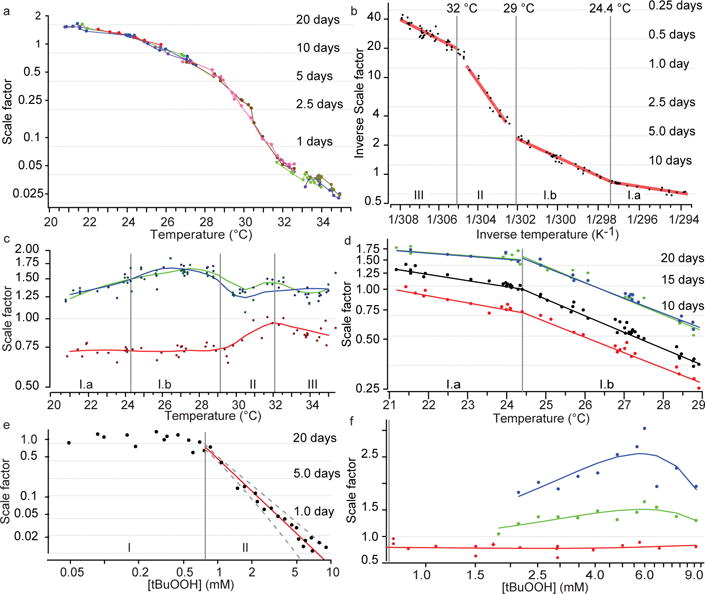
a, The magnitude of temporal scaling was estimated for wild-type populations held at fractional degree intervals across the range 20–35 °C. The scale factor λ of each population was estimated relative to a reference population at 25 °C. Grey lines mark the average lifespan of the reference population scaled by λ. Each replicate is shown as a separate colour, with each point corresponding to an aggregate population consisting of on average 130 individuals at the outset. b, The scale factor λ was determined for populations across the temperature range of a. The data points were fitted with a segmented Arrhenius model λ⁻¹(T) = p₀ exp(p₁/RT) (red). c, The magnitude of scaling produced by daf-16(mu86) (red), daf-2(e1368) (green), and age-1(hx546) (blue) alleles relative to wild type was estimated at each temperature considered (points). Solid curves represent trends across temperature as fitted by a Loess regression. d, The combined magnitude of scaling produced by each allele and change of temperature was estimated relative to a single wild-type population 24 °C; colours as in c. Regimes II and III are shown in Extended Data Fig. 7. e, Wild-type populations at 20 °C were exposed to a series of tBuOOH concentrations ranging from 0 to 10 mM. For each population, λ was calculated relative to an unexposed population (0 mM). Data for concentrations above 0.75 mM were fitted by the model λ ([tBuOOH]) = p₂([tBuOOH])^p3 (red), yielding p₂ = 0.47 ± 0.02 and p₃ = −1.86 ± 0.15. f, As in c, but for the tBuOOH dosage series.

Each scaling regime appears to correspond to a distinct molecular mechanism and barrier process dominating the timescale of ageing (Supplementary Table 1). Sharp decreases in lifespan have been observed to occur around 30 °C in Drosophila melanogaster²¹, hinting at a more general phenomenon in poikilotherms. Notably, this transition coincided with a deviation from temporal scaling of lifespan distributions (Fig. 1e and Extended Data Fig. 3). Intriguingly, the scaling across the breakpoint between regimes Ia and Ib suggested that temporal scaling need not be disrupted by a change in the molecular mechanisms dominating the timescale of ageing.

Quantifying the effects of temperature on mutant strains, we found that the elimination of DAF-16 shorted lifespan by a rescaling of 28% in regime Ia and 25% in Ib (Fig. 4c, d). The daf-16(mu86) population exhibited the same slope in scaling function as wild type in Ia, and differed only by about 5% across regime Ib, suggesting that the mechanisms mediating the temperature dependence of lifespan in regime I were not altered by elimination of DAF-16. In contrast, the hypomorphic alleles daf-2(e1368) and age-1(hx546) exhibit clear temperature-dependent effects across regime I (Fig. 4c, d). Both genes influence lifespan at 20 °C and 35 °C primarily by suppressing daf-16 activity²², which itself appears independent of temperature. Thus, daf-2(e1368) and age-1(hx546) alleles appear to be neomorphic in respect of the temperature dependence of their regulation of DAF-16.

We found that tBuOOH decreased lifespan at concentrations above 750 μM, with λ decreasing as a power law (Fig. 4e and Methods). This suggests an overall mass-action kinetics for the chain of events linking the direct targets of tBuOOH to the rescaling of the lifespan distribution. The distinct scaling functions of tBuOOH (power law) and temperature (multiple Arrhenius regimes) further suggest distinct molecular targets and mechanisms through which each type of intervention rescales the lifespan distribution.

As with temperature, the elimination of DAF-16 in the presence of tBuOOH reduced lifespan by a constant amount (Fig. 4f), 19.5 ± 8.8%, across all concentrations tested. Taken together with our temperature data in Fig. 4c, these results suggest that DAF-16 acts antagonistically but in parallel to the mechanisms through which tBuOOH and temperature shorten lifespan. DAF-16, tBuOOH, and temperature appear to affect ageing through their influence on risk determinants downstream of all three. For example, DAF-16 might attenuate or mitigate certain types of error or damage regardless of how the errors are created. The magnitude of temporal scaling produced both by daf-2(e1368) and by age-1(hx546) alleles varied across tBuOOH concentrations (Fig. 4g), which seems yet another aspect of a quantitative stress-dependent regulation of DAF-16 present in these strains but absent in wild type.

Disruption of daf-2, daf-16, hif-1, or hsf-1 produces distinct metabolic, cell-biological, and behavioural effects^15,23, as do changes in diet²⁴, temperature²⁵, and exposure to tBuOOH²⁶. Yet, temporal scaling arises independently of the molecular targets specific to each intervention and requires that all risk determinants be affected to the same extent. This suggests that ageing in C. elegans can be described in terms of a whole-organism state variable r that completely determines all-cause mortality (Extended Data Fig. 9). State variables familiar from other contexts include temperature, pressure, and entropy, all of which describe the behaviour of a system resulting from the collective action of its many constituent elements without reference to their nature. In the same way, the change of the state over time, r(t), describes the ageing process of C. elegans in terms of a collective action of all physiological determinants of risk. Where multiple risk determinants independently influence lifespan, temporal scaling requires that interventions simultaneously rescale, to an identical extent throughout life, the risk functions associated with each determinant (Supplementary Note 5.1). In models including dependencies among risk determinants, temporal scaling can emerge even when interventions act differentially across risk determinants (Supplementary Notes 5.2 and 5.3): dependencies can propagate the influence of interventions from one to all risk determinants, in effect producing a system-wide property that we call r(t).

The temporal scaling of lifespan distributions constrains the dynamics of the state variable r(t): the single stochastic process determining C. elegans lifespan must be invariant to timescale transformations and follow an average dynamics governed by a single effective rate constant: dr/dt = −k_rF(r), where F(r) is an unknown function of r that does not depend on k_r. In this formulation, temporal scaling arises when interventions change k_r into k_r/λ. These dynamics place constraints on any stochastic process proposed to describe organismal ageing, as its parameters must change in a coordinated fashion. For example, if r(t) were described by a biased random walk²⁷, the drift coefficient and the square of the diffusion coefficient must remain in a fixed proportion under intervention (Supplementary Note 6).

The idea that ageing is driven by changes in an organismal physiological state has been variously framed in terms of notions such as organization, vitality, organ reserve, or resilience^3,28,29. The temporal scaling across interventions justifies this notion, allowing an initial formalization. We note that any aspects of C. elegans physiology that change over time but do not influence lifespan, influencing ‘quality’ rather than ‘quantity’ of life, need not change in concert with r(t).

We know neither the physiological basis of the state r(t) nor the specific dynamics by which it changes with age. Yet, we can expect a broad set of lifespan determinants to affect only k_r, including minimally all determinants that influence lifespan exclusively through DAF-16 (refs 14, 30), HSF-1, or HIF-1, or through the mechanisms that mediate the effects of temperature and tBuOOH on lifespan. If most ageing mechanisms currently studied influence only k_r, then future studies directed at clarifying the physiological origins of r and its dynamics should identify novel ageing mechanisms F(r).

METHODS

Experimental methods

The following nematode strains were used: QZ0 (wild type (Bristol)), TJ1052 (age-1(hx546)II), and QZ120 (daf-2 (e1368)), QZ60 (daf-16(mu86)), QZ121 (hsf-1(sy441)), QZ414 (eat-2(ad1116)), ZG31 (hif-1(ia4)), and MQ1333 (nuo-6(qm200)).

Hermaphrodites were cultured under standard conditions^8,31, at either 20 °C or 25 °C as noted, on plates containing 100 μg ml⁻¹ ampicillin and seeded at an absorbance at 600 nm of 20 with the E. coli strain NEC937 B (OP50 ΔuvrA; KanR)³². Before seeding, all bacteria was irradiated in batch culture with 4 J m⁻² of 254-nm light in a UV Stratalinker (Stratagene). Age-synchronous cohorts were prepared by hypochlorite treatment³³. In strains exhibiting an increased variation in developmental time, in particular eat-2(ad1116) and nuo-6(qm200), developmentally synchronized L4 larvae were manually selected at the final stage of vulval maturation. To control for any effects of temperature on C. elegans development, all populations were held at 20 °C until their second day of adulthood, at which time they were exposed to the interventions described (unless otherwise stated). Individuals were randomly assigned groups by obtaining aliquots from populations suspended in M9 buffer. Automated lifespan experiments were run, blinded, and validated according to published methods⁸.

All populations were transferred on their second day of adulthood onto plates containing 22.5 μg ml⁻¹ nystatin (Sigma N3503) to prevent fungal growth and 27.5 μg ml⁻¹ 5-fluoro-2-deoxyuridine (FUDR, Sigma) to eliminate live progeny. Where live bacteria were used (Fig. 1h, i), 10 μg ml⁻¹ FUDR sufficed to eliminate live progeny.

Standard NGM agar plates were poured and dried according to published methods⁸. For tBuOOH assays, the compound was added to molten agar immediately before pouring. All plates containing tBuOOH were seeded and placed in a fume hood until the bacteria was absorbed, approximately 1 h. We found no evidence of time-dependent degradation of tBuOOH in solid agar plates, nor any effect of the tBuOOH degradation byproduct tbutanol on C. elegans lifespan (Extended Data Fig. 4), although evaporation of tBuOOH needed to be strictly controlled.

Scanner temperatures were measured using thermocouples (ThermoWorks USB-REF) mounted on the bottom of empty Petri dishes loaded onto each scanner. Scanners were given several hours to reach their stable operating temperature, at which point measurements were taken every 10 s. Because operating scanners exhibit small, regular oscillations in temperature⁸, the average of multiple cycles, each lasting 20 min, was taken.

Statistical methods

Population sizes

Supplementary Table 2 shows various summary statistics, including population size, for the population in each figure panel. No statistical methods were used to predetermine sample size. Initial experiments showed that populations larger than 500 individuals provided more robust survival estimates. Statistical power was estimated retrospectively (Supplementary Notes 2.2 and 6.3). Animals lost from observation were censored according to published methods⁸.

Replicates

All replicates described are biological replicates, performed in separate weeks using separate populations. All replicates performed in the laboratory yielding informative population sizes and meeting self-consistency standards (for example consistent results across multiple scanners⁸) are shown.

Single AFT regression (all figures)

Using our automated microscopy method⁸, a single, very large, homogeneous population must be distributed across multiple scanners. The local environment characteristic to each scanner can influence C. elegans lifespan. This influence can be measured and controlled using the same AFT model we use to quantify temporal scaling. In most cases, our AFT models take the form

$$\text{log}(y_i)=\beta X_i+{\epsilon }_i$$ (1)

where y_i is the lifespan of individual i, β is the parameter vector being estimated, and X_i is the categorical covariate coding for the label associated with each individual i. This label takes different values in different contexts, representing either the plate name (Figs 1, 2, 3b, d and 4b–f), scanner name (Fig. 4a), or animal genotype (Fig. 4c, f). We take the logarithm of lifespan, log(y_i), following the standard approach for evaluating multiplicative effects on lifespan, conceptually equivalent to stating that y_i = (βX_i)ε_i.

Each AFT regression model has an intercept that determines the ‘reference’ lifespan in relation to which all parameter vectors β are scaled. The intercept is implicitly determined by the particular categorical encoding scheme used for X_i. In Figs 1, 2 and 3b–d a ‘deviation’ coding is used, placing the intercept at the grand mean lifespan of all individuals. In Fig. 4, a dummy coding is used, placing the intercept at the mean lifespan of a specific reference group whose identity is noted in each case. The coding scheme used for the categorical variable has no effect on the value of model residuals ε_i and determines only the values of the AFT parameters β.

All AFT regression models were estimated via Buckley–James regression (included in the R³⁴ package RMS). In Figs 1a and 3b and Extended Data Fig. 5a, j, l, n, p, r, t, v ‘device-corrected death times’⁸ were calculated to remove obscuring effects of temperature variation between scanners on the aggregate hazard rate. A dummy encoding for X_i coded for the scanner on which each individual was observed. The model intercept was then added to the residuals ε_i.

In many panels, AFT residuals ε_i are grouped and plotted according to some experimental condition: by temperature in Figs 1c, d, e and 2l and Extended Data Fig. 4i; by tBuOOH concentration in Fig. 1g and Extended Data Fig. 4a; by bacterial treatment in Fig. 1i; and by genotype in Fig. 2d, e, f, j, k and Extended Data Fig. 4e, g, k, m, o, q, s, u, w. We emphasize that in each case, the experimental condition used to group plots is not a covariate in the AFT model. Instead, the single AFT categorical covariate codes for an experimental unit—plate or scanner name—as detailed above. In this way, any temporal rescaling produced by variation in environmental conditions across these units will be estimated and reflected in the parameter vector β, and its effects minimized on the residual times ε_i. These residuals are then grouped according to the experimental variable during subsequent analysis (Supplementary Note 2).

Single AFT regression for additive models (Fig. 3d–f, h and Extended Data Fig. 5b, e, l)

To account for temporal shifts in mortality statistics, Buckley–James regression (using the R³⁴ package RMS) was used to fit the model

$$y_i=\beta X_i+{\epsilon }_i$$ (2)

where X_i is the categorical covariate the initial (Fig. 3d–f and Extended Data Fig. 5b) temperature at which individual i was placed, the duration of time spent at that temperature (Extended Data Fig. 5d–g), or the number of switches used (Extended Data Fig. 5l). A ‘deviation’ coding was used (see equation (1)) in Fig. 3d and a dummy coding was used for Fig. 3e, f.

Significance (Figs 1 and 2)

The probability (P value) that the observed differences in lifespan between two populations are explained entirely by temporal scaling was estimated using the two-sided modified Kolmogorov–Smirnov test to identify heteroscedasticity among AFT residuals. This approach is described, with additional power analysis, in Supplementary Note 2.

Hierarchical clustering of survival curves (Extended Data Fig. 3)

A hierarchical clustering of survival curves was computed to identify groups of curves temporally rescaled in respect to each other. All pairs of populations were compared using the modified Kolmogorov–Smirnov test as described in Supplementary Note 2. The modified Kolmogorov–Smirnov distance (Supplementary Note 2) was used as the distance metric for clustering, using the R³⁴ hierarchical clustering implementation hclust.

Estimating hazard functions (Figs 1–3)

The time-dependent hazard rate was estimated through numerical differentiation of the Kaplan–Meier cumulative hazard estimate. To generate confidence bands for the true hazard rate under the assumption that it is locally smooth, death times were fitted with a piecewise-polynomial B-spline hazard model using the R³⁴ package bshazard³⁵.

Estimating the magnitude of temporal scaling across temperatures (Fig. 4a, b)

Buckley– James regression was used to fit the AFT model described in equation (1), with X_i as a categorical covariate coding the scanner name corresponding to each individual tested. By specifying a single scanner at 25 °C as the reference category of a reference coded categorical variable, the AFT parameter vector β becomes the best estimate of the scale factors relating lifespan on each scanner X_i to the 25 °C reference: S_X(t) = S_{25 °C}(λ⁻¹t).

Because the average temperature was measured for each scanner X_i, the corresponding λ can therefore be plotted in Fig. 4 a, b as a function of the temperature on the scanner that produced it.

Identifying distinct scaling regimes (Fig. 4b and Extended Data Figs 6 and 7a, b)

Because the temperature scaling of timescale λ did not appear uniform, we applied a linear segmented regression model using transformed variables to identify the number scaling regimes and estimate the boundaries between them. An Arrhenius model was fitted, assuming that within each segment

$${\lambda }^{-\mathit{1}}(T)=A{e}^{-B/T}$$ (3)

with λ(T) as the scale factor at temperature T, and A and B as pre-exponential and exponential Arrhenius constants, respectively. One or more breakpoints were incorporated at temperatures T = {C₁, C₂, …, C_i} to produce the segmented model

$$\mathit{\text{log}}({\lambda }^{-1}(T))=A-\frac{B_1}{T},T_{i-1}<T<T_i,i=1,\dots ,n$$ (4)

with T0 and Tn the fixed starting and end temperatures, respectively. A linear model was tested in the same fashion:

$${\lambda }^{-1}=A+B_{1}T,T_{i-1}<T<T_i,i=1,\dots ,n$$ (5)

Model parameters were estimated using the R³⁴ package ‘segmented’.

To generate best estimates for the B parameter within each Arrhenius scaling regime identified by segmented regression, death times within each regime were isolated and fitted using a nonlinear regression approach (R³⁴ package nls2). In all segmented and nonlinear regression models performed on λ values, each λ was weighted according to the size of the population used in the AFT regression from which the λ was estimated. Additional estimates of Arrhenius parameters were obtained following the approach described in equation (6).

Estimating the effect of mutations relative to wild type, across temperatures (Fig. 4c). To estimate the effect of mutant alleles on lifespan relative to wild type at each temperature, a separate AFT model as specified in equation (1) was run at each temperature considered. In each regression, X_i was specified as the genotype of individuals, with the categorical variable coded to use wild-type populations as the reference.

Characterizing the temperature dependence of mutant lifespan across temperatures, relative to wild type (Fig. 4d and Extended Data Fig. 7c). To identify differences in the temperature dependence of lifespan of mutants relative to wild type, we considered each thermal regime separately (regimes Ia and Ib in Fig. 4d and regimes II and III in Extended Data Fig. 7). We considered the model

$$\text{log}(y_i)={\beta }_g{X}_i+{\beta }_r{Y}_i+{\beta }_T{T}_i+{\beta }_x{X}_i{T}_i+{\epsilon }_i$$ (6)

where X_i is a categorical variable encoding for the genotype of the individual, Y_i is the biological replicate in which the individual was observed (animals originating from the same hypochlorite treatment in the same week have the same Y_i), and T_i is a continuous variable representing the temperature (in inverse degrees Kelvin) at which the individual was placed. The interaction term β_xX_iT_i captures any differential effect of temperature on the mutant strain relative to wild type. The null hypothesis, therefore, is that mutant individuals exhibit no difference in their response to temperature compared with wild-type individuals, which can be rejected if a significant non-zero value of β_x is observed, as calculated from the associated Wald Z score. The estimated model parameters are provided in Supplementary Table 3.

Multiple AFT regression across tBuOOH replicates (Fig. 4e). The absolute effect of tBuOOH on lifespan varies between replicates. Several factors may contribute to this, including a variation in temperature of the molten agar and the time spent pouring it, and a variation in duration time required to dry plates. The relative effect of different tBuOOH concentrations on lifespan within each replicate, however, appeared more robust. So, we estimated the relative effects of tBuOOH on lifespan using the multiple regression model

$$\text{log}(y_i)={\beta }_c{X}_i+{\beta }_r{Y}_i+{\epsilon }_j$$ (7)

with X_i as a categorical covariate coding for tBuOOH concentration, and Y_i as a categorical covariate coding for the replicate name. The tBuOOH covariate was coded such that the parameters β_c were relative to the 0 mM category. The biological replicate covariate was coded such that the parameters β_c were relative to a single reference replicate. In this way, the parameters β_c represent the best estimate of the relative effect of tBuOOH across replicates.

To determine the quantitative dependence of the scale factor on tBuOOH concentration, the values of β_r and the tBuOOH concentrations corresponding to each X_i were fitted by the polynomial model λ = b[tBuOOH]^a using the R³⁴ nonlinear regression package nls2.

A distinct statistical was attempted to confirm the above analysis in a different way. All death times were fitted with the single model

$$\text{log}(y_i)={\beta }_c{B}_i+{\beta }_r{Y}_i+{\beta }_x{Y}_i{B}_i+{\epsilon }_i$$ (8)

where B_i is the logarithm of the tBuOOH concentration to which each individual i was exposed, represented as a continuous covariate. This makes β_c the best estimate of the exponent of the power-law relationship between lifespan and tBuOOH concentration. Y_i is the biological replicate in which the individual was observed (animals originating from the same hypochlorite treatment in the same week have the same Y_i), and Y_iB_i is a cross term to identify any systematic differences between the effect of tBuOOH between replicates. The estimated model parameters are provided in Supplementary Table 3.

Single AFT regression on each tBuOOH replicate (Fig. 4e). To validate the multiple regression model described previously, the AFT model described in equation (1) was fitted separately on the data collected in each replicate, with X_i coded to correspond to the tBuOOH concentration. The dummy variables for the tBuOOH covariate were set up such that scale factors were relative to the 0 mM control group. Using these cofactors, the R³⁴ nonlinear regression package nls2 was used to fit the polynomial relationship λ = b[tBuOOH]^a for each replicate.

Estimating the effect of genotype relative to wild type, across tBuOOH concentrations (Fig. 4f). To measure the effect of mutant alleles on lifespan across tBuOOH concentrations, a separate AFT model as specified in equation (1) was run on each data set collected at each concentration. In each regression, X_i was specified as the genotype of individuals, with the categorical variable coded to use wild-type populations as the model intercept.

Extended Data

Extended Data Figure 1. Characterizing the shape of wild-type lifespan distributions at 20 °C.

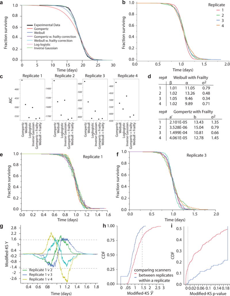
a, The AFT residuals corresponding to the 20 °C wild-type population presented in Fig. 1 were fitted with a variety of parametric distributions (Supplementary Note 1.4). Fits made to AFT residuals, as opposed to absolute death times, are much less sensitive to any environmental heterogeneity existing between plates and scanners (Statistical methods). b, The AFT residuals of four additional replicates at 20 °C to assess deviations from temporal scaling between replicates. c, The Akaike information criterion (AIC) was calculated for the each parametric fit of each replicate’s AFT residuals shown in panel b. Lower AIC values suggest preferred models. d, The parameters of Gompertz and Weibull distributions with frailty corrections are listed; both distributions were good fits across all replicates. e, f, The survival curves of populations collected in two biological replicates are shown, with one curve for individuals observed on each of 10 and 6 scanners respectively. g, The modified Kolmogorov–Smirnov Y(t) (Supplementary Note 2) is plotted for comparisons between replicate 1 and all others. Pairs for which Y(t) > 1.51 for some t exhibit statistically significant deviations from perfect scaling. In this case every replicate differed significantly from the first replicate. h, The distribution of modified Kolmogorov–Smirnov score scores, Ῡ, is plotted for comparisons between scanners within a replicate (blue) and between scanners in different replicates (red). Differences between replicates were larger than differences with replicates, suggesting that distance between survival curves observed between scanners cannot alone explain the distance between survival curves observed between replicates. i, The P values corresponding to each Ῡ are shown, with values P > 0.01 considered statistically significant (grey line).

Extended Data Figure 2. Apparent deviations from temporal scaling are observed when single replicates are performed at each temperature.

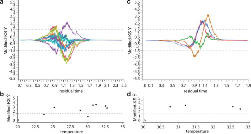
a, For the data shown in Fig. 1a, the modified Kolmogorov–Smirnov test Y(t) was calculated for AFT residuals (Statistical methods and Supplementary Note 2) to compare the reference population at 20 °C with populations held at each of the other temperatures. Pairs for which Y(t) > 1.51 for some t (grey dashed line) exhibit significant deviations from perfect scaling. b, The modified Kolmogorov–Smirnov test scores Ῡ, corresponding to the maximum absolute value of Y(t) observed at any time t, are shown for the comparisons in a, highlighting the statistical deviations observed between independent replicates performed at different temperatures. c, d, The same statistics were calculated when comparing all populations above 30 °C with the population at 30 °C.

Extended Data Figure 3. Independent replicates demonstrate that apparent deviations from temporal scaling within low- and high-temperature regimes arise from uncontrolled environmental variation.

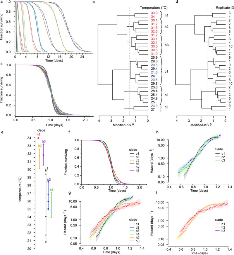
The lifespan of individuals from populations housed between 20 °C and 34 °C were collected using the lifespan machine (also shown in Fig. 4a, b). To characterize the effects of any uncontrolled experimental conditions specific to individual replicates, and identify any effects of temperature consistent across replicates, we divided the full temperature range into 2 °C intervals. Each 2 °C interval contained lifespan data collected in either two or three independent replicate experiments performed in separate weeks. a, Within each 2 °C range, all death times were fitted by an AFT regression model using plate name as a categorical covariate (Statistical methods). The device-corrected death times (the residual time plus model intercept⁸) were plotted, highlighting the changes in survival curve shape between replicates within each 2 °C range. b, All deaths across all temperatures were then fitted by a single AFT regression model with plate name as the categorical covariate. AFT residuals were grouped according to their replicate name and temperature range, and plotted to highlight the deviations from temporal scaling across all replicates at all temperatures. c, The modified Kolmogorov–Smirnov test (Supplementary Note 2) was applied on each pair of curves shown in b. The resulting Kolmogorov–Smirnov Ῡ was used as a distance metric with which to perform a hierarchical clustering, shown as a dendrogram with each replicate population labelled by the temperature at which it lived. In this dendogram, populations exhibiting smaller deviations from temporal scaling will have fewer branches between them. Clades that contain statistically significant deviations from temporal scaling have branches extending beyond the dashed grey line, indicating that Ῡ > 1.51 between branches. Six statistically distinct groups were identified, three above 30 °C and three below. d, The same dendogram is shown with populations labelled according to the name of the replicate in which they were collected. Populations collected in single replicates did not fall into single clades. This suggests that some environmental factor variable within replicates, distinct from the particular temperature at which populations were placed, produced the observed deviations from temporal scaling. e, The statistically distinct clades identified by hierarchical clustering (c) are plotted on a temperature scale. Clades overlap at all temperatures except the 30 °C boundary, suggesting that only the 30 °C transition represents a true temperature-dependent deviation from temporal scaling. f, The aggregate survival curves containing the AFT residuals of all individuals in each statistically distinct clade are compared, to highlight the differences in shape between clades. g, The hazard rate plot of the AFT residuals of all individuals in each statistically distinct clade. h, Break out of the hazards for only for low-temperature populations. i, Break out of the hazards for only high-temperature populations.

Extended Data Figure 4. Additional survival curves and hazard plots.

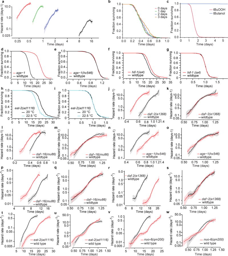
a, The hazard rates corresponding to the tBuOOH survival data presented in Fig. 1: 0 mM (black), 1.5 mM (blue), 3 mM (green), and 6 mM (red). b, To test for any effects of tBuOOH degradation and evaporation on lifespan, 9 mM tBuOOH plates were prepared and placed at 4 °C. On 4 consecutive days, a subset of plates were seeded with ultraviolet-inactivated bacteria and placed without C. elegans on scanners operating at 20 °C. In this way, four groups of plates were created, corresponding to 0, 1, 2, and 3 days of cumulative exposure to standard scanner conditions during which tBuOOH degradation and evaporation could potentially occur. A single age-synchronous population of 2-day-old adult C. elegans was then simultaneously distributed across all plates. The remaining lifespan of all worms at 20 °C was recorded using the lifespan machine. c, In a separate experiment, plates were prepared containing either 3 mM tBuOOH or 3 mM t-butanol, a degradation product of tBuOOH. On t-butanol, only a trivial fraction of individuals had died by the fifth day, so the experiment was terminated. d, e, The survival of wild-type and age-1(hx546) populations at 25 °C. f, g, The lifespan and AFT residuals for hif-1(ia4) and wild-type populations, calculated as in Fig. 2. h, i, The lifespan and AFT residuals for eat-2(ad1116) at 20 ° and 22.5 °C. j–o, Age-synchronous mutant (red) and wild-type (black) populations were raised at 25 °C and then transferred to 33 °C on their second day of adulthood, where they remained until death. For each population at 33 °C, the hazard rate was estimated from the death times (j, l, n). The hazard rate was also estimated from the residuals of the AFT regression model log(y_i) = βx_i + ε_i with genotype as a single categorical covariate (k, m, o). p, q, The hazard functions of death times and AFT residuals corresponding to the daf-16(mu86) data presented in Fig. 1. r, s, The hazard functions of death times and AFT residuals corresponding to the daf-2(1368) data presented in Fig. 1. t, u, The hazard functions of death times and AFT residuals corresponding to the eat-2(ad1116) data presented in Fig. 1. v, w, The hazard functions of death times and AFT residuals corresponding to the nuo-6(qm200) data presented in Fig. 1.

Extended Data Figure 5. Additional temperature shift data.

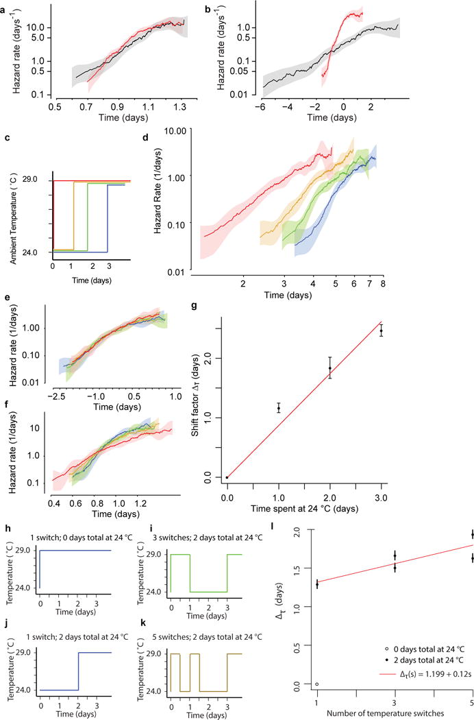
a, As a control for the temperature shift experiment shown in Fig. 3, the same regression as in Fig. 3c was run to test for temporal scaling between populations always held at 24 °C (black) and those always held at 29 °C (red). The residuals ε_i are plotted as hazard functions. b, The same regression as in Fig. 3 was run for the same populations as b here, to test for temporal shifts. c, To test for the effects of different durations spent at 24 °C before transfer to 29 °C. Age-synchronous, wild-type animals were grown at 20 °C and then transferred on their second day of adulthood to 24 °C. Subsets of these animals were then transferred to 29 °C on each of 3 consecutive days. d, For each population, the remaining lifespan was observed and the hazard functions estimated. All death times represent the number of days after the second day of adulthood. e, The residuals from a regression model with the duration at 24 °C as an additive categorical covariate y_i = βx_i + ε_i. f, The residuals from a regression model with the duration at 24 °C as a proportional covariate log(y_i) = βx_i + ε_i. g, The shift values β=Δ_τ of the additive model are plotted along with a linear fit. h, To test for the effect of rapid temperature changes on lifespan, age-synchronous individuals were raised at 20 °C. On their second day of adulthood, a subset was transferred to 29 °C. i, Another subset of individuals remained at 24 °C for 2 days, after which they were transferred to 29 °C. j, Another subset was transferred to 29 °C, but switched down from 29 °C to 24 °C and then back again to 29 °C (filled circle; three shifts). k, A final subset was switched down and back twice (filled circle; five shifts). Note that all populations spent the same total duration at 29 °C, except for the aforementioned control population that was never switched. l, The data were fitted with an additive regression model y_i = βx_i + ε_i with the number of switchings as a categorical covariate. The encoding of this covariate was set so that all β=Δ_τ represent each subpopulation’s change in lifespan relative to the control population that was never switched.

Extended Data Figure 6. Identifying the number of thermal regimes, and the boundaries between them.

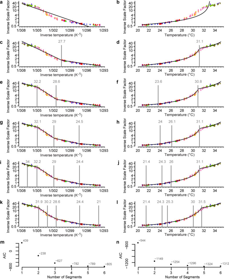
The thermal scaling data presented in Fig. 4a were fitted with a segmented regression model (Statistical methods) assuming that λ⁻¹ relates to temperature either following an Arrhenius relationship, λ⁻¹(T) = p₀ exp(p₁/RT) (a, c, e, g, i, k) or a linear relationship, λ⁻¹ (T) = p₀ T + p₁ (b, d, f, h, j, l; Statistical methods). The model fits are plotted in black, with model breakpoints shown as vertical lines. Colours correspond to independent replicates. Each model was fitted assuming a single segment (a, b), two segments (c, d), three segments (e, f), four segments (g, h), five segments (i, j), or six segments (k, l). m, The AIC corresponding to each number of segments for the Arrhenius is plotted. n, The AIC for the linear model is plotted. Because the the Arrhenius and linear models models are fit to distinct data sets (log-transformed and untransformed scale factors respectively, and inverse temperature and untransformed temperatures, respectively), AIC values cannot be compared between Arrhenius and inverse time models. Regime I can be adequately described either by one linear regime or two piecewise Arrhenius regimes, Ia and Ib. Across multiple replicates, the linear 1/T model consistently underestimated C. elegans lifespan around 25 °C, leading us to favour the piecewise Arrhenius model (See Extended Data Figure 6). Regimes II and III involve temperature ranges that are too narrow to distinguish between Arrhenius and linear models. Above 35.5 °C, lifespan is too short to be accurately measured with our time-lapse technique.

Extended Data Figure 7. Additional data for the regression models in Fig. 4b, d.

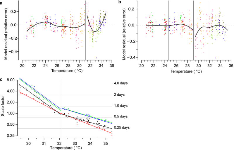
The residuals of the linear model (a) shown in Extended Data Fig. 6f. The residuals of the Arrhenius Arrhenius model (b) shown in Fig. 4b are depicted, showing the deviation of the predicted value from the empirical data across each regime. Residuals are presented in the form of relative error, the ratio between the model’s prediction and the empirical measurement. c, As in Fig. 4d, the response of each genotype, wild type (black), daf-16(mu86) (red), daf-2(e1368) (green), and age-1(hx546) (blue) to changes of temperature was estimated (Statistical methods) in regime II and in regime III.

Extended Data Figure 8. The potential effects of heterogeneity at 33 °C.

a, Fifty-six thousand samples were drawn from the distribution of frailty effects Z^−1/α as described in Supplementary Note 3.1, where Z is a random variable, sampled from an inverse-gamma distribution with mean 1 and a standard deviation corresponding to the value estimated from experimental data. Samples were drawn using the σ² estimated for populations at 25 °C (black) and at 33 °C (red), corresponding to the data presented in Fig. 1d. The probability density function of each population is shown, which can be interpreted as the variable effect of unknown factors on lifespan across individuals at each temperature. b, At each temperature, 25 °C (black) and at 33 °C (red), we estimated the distribution of temperature changes required to produce the distribution of frailties shown in a. This was accomplished using temperature scaling function shown in Fig. 4b. c, Fifty-six thousand random samples were drawn from the transformed inverse gamma distribution of Z^−1/α with σ² set to the estimate of Δσ² in equation (15) of Supplementary Note 3.2. Each sample was multiplied by a death time drawn (with replacement) from the set of 25 °C residual times of Fig. 1d, shown here in black. These products constitute a ‘transformed’ set of death times, corresponding to the 25 °C residuals with additional frailty synthetically introduced. The residual death times of animals placed at 33 °C are shown for comparison (red).

Extended Data Figure 9. The organization of lifespan determinants (schematic).

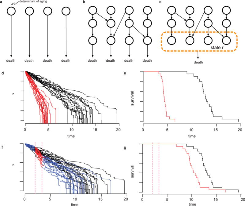
a, A set of molecular determinants of risk of death (open circles) do not interact, as is assumed in a competing risks and weakest link models. b, Risk determinants might interact (arrows) in complex ways to determine lifespan. In this schematic, each risk of death is still determined by separate factors. c, Our data on temporal scaling suggest that the set of molecular determinants that determine risk of death (within the dotted circle) must change in concert when exposed to interventions in ageing. This set is therefore well described by a single state variable r. d, A cartoon of the stochastic decline of such a state variable (generated from the dependency model discussed in Supplementary Note 5.2). Each trajectory represents the values of r over time for each individual in a population. Interventions affect the dynamics of the state decline by rescaling the average dynamics of exposed individuals (red lines), which produces (e) a rescaling of the resultant survival curve. f, Transient interventions in young adults (applied within the red dotted vertical lines) transiently rescale the average dynamics, leading to (g) a shift in the lifespan distribution.

References

- 1.Pincus Z, Smith-Vikos T, Slack FJ. MicroRNA predictors of longevity in Caenorhabditis elegans. PLoS Genet. 2011;7:e1002306. doi: 10.1371/journal.pgen.1002306. [DOI] [PMC free article] [PubMed] [Google Scholar]
- 2.Herndon LA, et al. Stochastic and genetic factors influence tissue-specific decline in ageing C. elegans. Nature. 2002;419:808–814. doi: 10.1038/nature01135. [DOI] [PubMed] [Google Scholar]
- 3.Shaw RF, Bercaw BL. Temperature and life-span in poikilothermous animals. Nature. 1962;196:454–457. doi: 10.1038/196454a0. [DOI] [PubMed] [Google Scholar]
- 4.Mair W, Goymer P, Pletcher SD, Partridge L. Demography of dietary restriction and death in Drosophila. Science. 2003;301:1731–1733. doi: 10.1126/science.1086016. [DOI] [PubMed] [Google Scholar]
- 5.Wu D, Rea SL, Cypser JR, Johnson TE. Mortality shifts in Caenorhabditis elegans: remembrance of conditions past. Aging Cell. 2009;8:666–675. doi: 10.1111/j.1474-9726.2009.00523.x. [DOI] [PMC free article] [PubMed] [Google Scholar]
- 6.Conti B, et al. Transgenic mice with a reduced core body temperature have an increased life span. Science. 2006;314:825–828. doi: 10.1126/science.1132191. [DOI] [PubMed] [Google Scholar]
- 7.Lithgow GJ, White TM, Melov S, Johnson TE. Thermotolerance and extended life-span conferred by single-gene mutations and induced by thermal stress. Proc Natl Acad Sci USA. 1995;92:7540–7544. doi: 10.1073/pnas.92.16.7540. [DOI] [PMC free article] [PubMed] [Google Scholar]
- 8.Stroustrup N, et al. The Caenorhabditis elegans lifespan machine. Nature Methods. 2013;10:665–670. doi: 10.1038/nmeth.2475. [DOI] [PMC free article] [PubMed] [Google Scholar]
- 9.Johnson TE, Wu D, Tedesco P, Dames S, Vaupel JW. Age-specific demographic profiles of longevity mutants in Caenorhabditis elegans show segmental effects. J Gerontol A. 2001;56:B331–B339. doi: 10.1093/gerona/56.8.b331. [DOI] [PubMed] [Google Scholar]
- 10.Swindell WR. Accelerated failure time models provide a useful statistical framework for aging research. Exp Gerontol. 2009;44:190–200. doi: 10.1016/j.exger.2008.10.005. [DOI] [PMC free article] [PubMed] [Google Scholar]
- 11.Vaupel JW, Manton KG, Stallard E. The impact of heterogeneity in individual frailty on the dynamics of mortality. Demography. 1979;16:439–454. [PubMed] [Google Scholar]
- 12.Martin GM, Austad SN, Johnson TE. Genetic analysis of ageing: role of oxidative damage and environmental stresses. Nature Genet. 1996;13:25–34. doi: 10.1038/ng0596-25. [DOI] [PubMed] [Google Scholar]
- 13.Tullet JM, et al. Direct inhibition of the longevity-promoting factor SKN-1 by insulin-like signaling in C. elegans. Cell. 2008;132:1025–1038. doi: 10.1016/j.cell.2008.01.030. [DOI] [PMC free article] [PubMed] [Google Scholar]
- 14.Landis JN, Murphy CT. Integration of diverse inputs in the regulation of Caenorhabditis elegans DAF-16/FOXO. Dev Dyn. 2010;239:1405–1412. doi: 10.1002/dvdy.22244. [DOI] [PMC free article] [PubMed] [Google Scholar]
- 15.Hsu AL, Murphy CT, Kenyon C. Regulation of aging and age-related disease by DAF-16 and heat-shock factor. Science. 2003;300:1142–1145. doi: 10.1126/science.1083701. [DOI] [PubMed] [Google Scholar]
- 16.Leiser SF, Begun A, Kaeberlein M. HIF-1 modulates longevity and healthspan in a temperature-dependent manner. Aging Cell. 2011;10:318–326. doi: 10.1111/j.1474-9726.2011.00672.x. [DOI] [PMC free article] [PubMed] [Google Scholar]
- 17.Kirkwood TB, Shanley DP. Food restriction, evolution and ageing. Mech Ageing Dev. 2005;126:1011–1016. doi: 10.1016/j.mad.2005.03.021. [DOI] [PubMed] [Google Scholar]
- 18.Garigan D, et al. Genetic analysis of tissue aging in Caenorhabditis elegans: a role for heat-shock factor and bacterial proliferation. Genetics. 2002;161:1101–1112. doi: 10.1093/genetics/161.3.1101. [DOI] [PMC free article] [PubMed] [Google Scholar]
- 19.Lakowski B, Hekimi S. The genetics of caloric restriction in Caenorhabditis elegans. Proc Natl Acad Sc USA. 1998;95:13091–13096. doi: 10.1073/pnas.95.22.13091. [DOI] [PMC free article] [PubMed] [Google Scholar]
- 20.Suda H, Sato K, Yanase S. Timing mechanism and effective activation energy concerned with aging and lifespan in the long-lived and thermosensory mutants of Caenorhabditis elegans. Mech Ageing Dev. 2012;133:600–610. doi: 10.1016/j.mad.2012.07.007. [DOI] [PubMed] [Google Scholar]
- 21.Atlan H, Miquel J, Helmle LC, Dolkas CB. Thermodynamics of aging in Drosophila melanogaster. Mech Ageing Dev. 1976;5:371–387. doi: 10.1016/0047-6374(76)90035-x. [DOI] [PubMed] [Google Scholar]
- 22.Libina N, Berman JR, Kenyon C. Tissue-specific activities of C. elegans DAF-16 in the regulation of lifespan. Cell. 2003;115:489–502. doi: 10.1016/s0092-8674(03)00889-4. [DOI] [PubMed] [Google Scholar]
- 23.Murphy CT, et al. Genes that act downstream of DAF-16 to influence the lifespan of Caenorhabditis elegans. Nature. 2003;424:277–283. doi: 10.1038/nature01789. [DOI] [PubMed] [Google Scholar]
- 24.Walker G, Houthoofd K, Vanfleteren JR, Gems D. Dietary restriction in C. elegans: from rate-of-living effects to nutrient sensing pathways. Mech Ageing Dev. 2005;126:929–937. doi: 10.1016/j.mad.2005.03.014. [DOI] [PubMed] [Google Scholar]
- 25.McColl G, et al. Insulin-like signaling determines survival during stress via posttranscriptional mechanisms in C. elegans. Cell Metab. 2010;12:260–272. doi: 10.1016/j.cmet.2010.08.004. [DOI] [PMC free article] [PubMed] [Google Scholar]
- 26.Oliveira RP, et al. Condition-adapted stress and longevity gene regulation by Caenorhabditis elegans SKN-1/Nrf. Aging Cell. 2009;8:524–541. doi: 10.1111/j.1474-9726.2009.00501.x. [DOI] [PMC free article] [PubMed] [Google Scholar]
- 27.Aalen OO, Gjessing HK. Understanding the shape of the hazard rate: a process point of view. Stat Sci. 2001;16:1–22. [Google Scholar]
- 28.Medawar PB. An Unsolved Problem of Biology: An Inaugural Lecture Delivered at University College London. H.K. Lewis; 1951. [Google Scholar]
- 29.Gladyshev VN. The origin of aging: imperfectness-driven non-random damage defines the aging process and control of lifespan. Trends Genet. 2013;29:506–512. doi: 10.1016/j.tig.2013.05.004. [DOI] [PMC free article] [PubMed] [Google Scholar]
- 30.Samuelson AV, Carr CE, Ruvkun G. Gene activities that mediate increased life span of C. elegans insulin-like signaling mutants. Genes Dev. 2007;21:2976–2994. doi: 10.1101/gad.1588907. [DOI] [PMC free article] [PubMed] [Google Scholar]
- 31.Stiernagle T. The C. elegans Research Community, editor. WormBook. http://dx.doi.org/10.1895/wormbook.1.101.1 (February 11, 2006)
- 32.Baeriswyl S, et al. Modulation of aging profiles in isogenic populations of Caenorhabditis elegans by bacteria causing different extrinsic mortality rates. Biogerontology. 2010;11:53–65. doi: 10.1007/s10522-009-9228-0. [DOI] [PubMed] [Google Scholar]
- 33.Wilkinson DS, Taylor RC, Dillin A. Analysis of aging in Caenorhabditis elegans. Methods Cell Biol. 2012;107:353–381. doi: 10.1016/B978-0-12-394620-1.00012-6. [DOI] [PubMed] [Google Scholar]
- 34.R Core Team. R: a language and environment for statistical computing. R Foundation for Statistical Computing; 2013. [Google Scholar]
- 35.Rebora P, Salim A, Reilly M. Bshazard: a flexible tool for nonparametric smoothing of the hazard function. R J. 2014;6:114–122. [Google Scholar]
Associated Data
This section collects any data citations, data availability statements, or supplementary materials included in this article.