Multiscale Modeling of Double-Helical DNA and RNA: A Unification through Lie Groups

Abstract

Several different mechanical models of double-helical nucleic-acid structures that have been presented in the literature are reviewed here together with a new analysis method that provides a reconciliation between these disparate models. In all cases, terminology and basic results from the theory of Lie groups are used to describe rigid-body motions in a coordinate-free way, and when necessary, coordinates are introduced in a way in which simple equations result. We consider double-helical DNAs and RNAs which, in their unstressed referential state, have backbones that are either straight, slightly precurved, or bent by the action of a protein or other bound molecule. At the coarsest level, we consider worm-like chains with anisotropic bending stiffness. Then, we show how bi-rod models converge to this for sufficiently long filament lengths. At a finer level, we examine elastic networks of rigid bases and show how these relate to the coarser models. Finally, we show how results from molecular dynamics simulation at full atomic resolution (which is the finest scale considered here) and AFM experimental measurements (which is at the coarsest scale) relate to these models.

Graphical abstract

1. INTRODUCTION

DNA and RNA double helices are fairly stiff and are often treated as homogeneous elastic rods. However, double helices with different base compositions are not structurally or dynamically equal, thus leading to studies of rigid-base and rigid-base-pair models. In this paper, we focus on a unified Lie-group framework that reconciles the most typical levels of coarse-graining in DNA and RNA modeling—from molecular dynamics, to rigid-base, to rigid-base-pair, to elastic filament models. We provide a survey of common models recast in terms of Lie groups while also demonstrating new methods for reconciliation between the disparate models. Figure 1 illustrates the different levels of modeling that are compared and contrasted in this paper, and some of the ways that they are related. It also depicts several connections that are made between these models and experiments/simulations that have been performed, namely, molecular dynamics simulations and measurements using atomic force microscopy.

Figure 1.

An overview of the models explored and some of the connections made between them.

The structure of DNA and RNA plays an important role in the function of these molecules, and hence has been studied extensively.^1,2 Different double helix structures can allow for different compaction ratios within the cell, initiate supercoiling, affect the local concentration of the solution (e.g., by interacting with ions and water), and create a variety of nanostructures. Studying the properties of these double helices can help determine these structure–function relationships. A standard helical structure and its implementation into nanostructures is shown in Figure 2. Such structures, as well as naturally occurring DNAs and RNAs, consist of a combination of double-helical regions, stiff bends, and/or regions of increased flexibility (bulges and defects). The models and methods that we present here are general enough to address all of these scenarios.

Figure 2.

Two examples of how helical RNA can be used to create nanostructures.

Over the past few decades, experimental and theoretical studies of the mechanical behavior of double-stranded DNA have focused on long length scales (>100 nm). The most popular theoretical method is the elastic-filament model that treats the macromolecule as an inextensible elastic rod, and attributes to its bending deformations a classical elastic energy cost (Hooke’s law). Its success can be attributed to its simplicity and its successful description of experiments such as force spectroscopy on single DNA molecules.^3–5 However, for short and intermediate length scales, the elastic-filament model using DNA stretching, atomic force microscopy (AFM), and other methods has been largely insensitive to the details of mechanics crucial for cellular function, DNA packaging, transcription, gene regulation, and viral packaging.^6–10

To further evaluate the elastic properties of DNA, DNA sequence-dependent flexibility has been examined.^11–13 Sequence-dependent local (base-pair step) force fields and chain properties have been inferred from molecular dynamics simulations and compared with results from other techniques. Accumulating evidence shows that there are preferential DNA binding sequences and significant variability depending on sequence. For example, it was shown that alternating AT repeats are 20% more flexible than control sequences.¹⁴ Interestingly, studies on RNA elasticity models (of varying length scales) and RNA sequence-dependent flexibility are few, especially considering the greater wealth of structural features available.

In the emerging field of nanotechnology, it is becoming very important to know the properties of these biological motifs, especially when designing nanostructures.¹⁵ For example, if the desired nanostructure is a very rigid cube, a natural building block for the sides of the cube would be the double helix. However, it would be useful to know the stiffness parameters for helices with different base compositions so that the stiffest helix could be selected for structure. This is one of many scenarios in which coarse-grained mechanical models can be used. Bridging different length scales is facilitated by methodologies such as those presented here.

The remainder of this paper is organized as follows. Section 2 provides a brief review of the Lie-group methods that are common to all four models of DNA detailed in this paper. Section 3 reviews the generalized elastic filament or worm-like chain model in which local stiffness can be completely anisotropic, and the baseline backbone shape can be an arbitrary curve. The worm-like chain model is then applied to DNA with a drug induced bend as a special case. Section 4 describes the bi-rod model in which a double-helical nucleic acid structure is viewed as two intertwined elastic rods, and reconciles this model with the single elastic filament case using properties of the classical Ornstein–Uhlenbeck stochastic process. The rigid-base-pair model discussed in section 5 uses a rigid body to represent each base pair in double-stranded DNA or RNA. Predictions of this model with fine-grained molecular dynamics simulations are shown to be consistent. The final model detailed in section 6 represents each of the bases of DNA and RNA as rigid bodies connected by a network of elastic constraints to create a double-helical structure. Section 7 provides conclusions and discusses avenues for future work.

2. A LIE-GROUP TREATMENT OF RIGID-BODY MOTIONS

The set of rigid-body motions is denoted in this paper as G = SE(3) (the special or proper Euclidean motion group in three space). Any g ∈ G can be faithfully represented with a 4 × 4 homogeneous transformation matrix of the form

$$g=\left(\begin{array}{ll}R& \mathbf{t}\\ {\mathbf{0}}^T& 1\end{array}\right)=\left(\begin{array}{ll}{\mathbb{I}}_3& \mathbf{t}\\ {\mathbf{0}}^T& 1\end{array}\right)\left(\begin{array}{ll}R& \mathbf{0}\\ {\mathbf{0}}^T& 1\end{array}\right)=\text{trans}(\mathbf{t})\text{rot}(R)$$ (1)

where R ∈ SO(3) (the special orthogonal group) is a 3 × 3 rotation matrix, ${\mathbb{I}}_n$ is the n × n identity matrix, t is a translation vector, and 0^T = [0, 0, 0] is a row of zeros. The first matrix on the right-hand side of eq 1 is a pure translation, and the second is a pure rotation. The set of all such transformations together with the operation of matrix multiplication (which sometimes is denoted as ○) forms a group, (G, ○). Often we will suppress the ○ and denote the group product as the juxtaposition of group elements unless it is useful to emphasize it.

Every such rigid-body motion can be parametrized using the matrix exponential as

$$g=\exp (X)\text{where}X={\displaystyle \sum _{i=1}^6{x}_i{E}_i}\text{and}\mathbf{x}={[x_1,\dots ,x_6]}^T$$ (2)

The matrix exponential can be defined using the Taylor series such that

$$\exp (X)=\mathbb{I}+X+\frac{1}{2}{X}^2+\frac{1}{3!}{X}^3+\dots$$

The matrix logarithm can be used as the inverse of the matrix exponential so that

$$\log (\exp (X))=X$$

It should be noted that log(g) is not well-defined everywhere, but it can be used for nearly every g ∈ SE(3). Here

$$\begin{array}{ll}{E}_1=\left(\begin{array}{llll}0\hfill & 0\hfill & 0\hfill & 0\hfill \\ 0\hfill & 0\hfill & -1\hfill & 0\hfill \\ 0\hfill & 1\hfill & 0\hfill & 0\hfill \\ 0\hfill & 0\hfill & 0\hfill & 0\hfill \end{array}\right);& E_2=\left(\begin{array}{llll}0\hfill & 0\hfill & 1\hfill & 0\hfill \\ 0\hfill & 0\hfill & 0\hfill & 0\hfill \\ -1\hfill & 0\hfill & 0\hfill & 0\hfill \\ 0\hfill & 0\hfill & 0\hfill & 0\hfill \end{array}\right);\\ E_3=\left(\begin{array}{llll}0\hfill & -1\hfill & 0\hfill & 0\hfill \\ 1\hfill & 0\hfill & 0\hfill & 0\hfill \\ 0\hfill & 0\hfill & 0\hfill & 0\hfill \\ 0\hfill & 0\hfill & 0\hfill & 0\hfill \end{array}\right);& E_4=\left(\begin{array}{llll}0\hfill & 0\hfill & 0\hfill & 1\hfill \\ 0\hfill & 0\hfill & 0\hfill & 0\hfill \\ 0\hfill & 0\hfill & 0\hfill & 0\hfill \\ 0\hfill & 0\hfill & 0\hfill & 0\hfill \end{array}\right);\\ E_5=\left(\begin{array}{llll}0\hfill & 0\hfill & 0\hfill & 0\hfill \\ 0\hfill & 0\hfill & 0\hfill & 1\hfill \\ 0\hfill & 0\hfill & 0\hfill & 0\hfill \\ 0\hfill & 0\hfill & 0\hfill & 0\hfill \end{array}\right);& E_6=\left(\begin{array}{llll}0\hfill & 0\hfill & 0\hfill & 0\hfill \\ 0\hfill & 0\hfill & 0\hfill & 0\hfill \\ 0\hfill & 0\hfill & 0\hfill & 1\hfill \\ 0\hfill & 0\hfill & 0\hfill & 0\hfill \end{array}\right);\end{array}$$

are the infinitesimal generators of the group.

The linear vector space spanned by {E_i}, together with the matrix commutator operation [X, Y] = XY − YX, defines the Lie algebra $\mathcal{G}=se(3)$ associated with the Lie group G = SE(3).

The explicit closed-form expression for the matrix exponential in eq 2 is known,¹⁶ but the most relevant fact for our presentation is that when ‖x‖ ≪ 1, $\exp (X)\approx {\mathrm{I}}_4+X$.

Let g(s) be a reference frame that evolves with curve parameter s and ġ(s) ≐ dg/ds (throughout our formulation, the curve parameter, s, takes the place that “time” would normally have in formulations of rigid-body mechanics). The composite translational and angular “velocity” corresponding to g(s) = exp X(s) and described in the moving reference frame is extracted from

$$g^{-1}\dot{g}=\left(\begin{array}{ll}{R}^T\dot{R}& R^T\dot{\mathbf{t}}\\ {\mathbf{0}}^T& 0\end{array}\right)={\displaystyle \sum _{i=1}^6{\xi }_i(s)E_i}$$

using the “∨” operator, which is the unique linear operator such that

$$E_i^{\vee }={\mathbf{e}}_i$$

the ith natural unit basis vector for ℝ⁶. Then,

${(g^{-1}\dot{g})}^{\vee }=\xi (s)$

The opposite operation of ∨ is

$$\widehat{\xi }(s)=g^{-1}\dot{g}={\displaystyle \sum _{i=1}^6{\xi }_i{E}_i}$$

It is often convenient to decompose ξ into its angular (ω) and translational (v) parts as

$$\xi =\left(\begin{array}{l}\mathit{\omega }\\ \mathbf{v}\end{array}\right)$$

Two important adjoint matrices are Ad(g) and ad $(\widehat{\xi })$ which for SE(3) and se(3) are defined as follows

$$\text{Ad}(g)=\left(\begin{array}{ll}R& O\\ TR& R\end{array}\right)\text{and}\text{ad}(\widehat{\xi })=\left(\begin{array}{ll}\mathrm{\Omega }& O\\ V& \mathrm{\Omega }\end{array}\right)$$ (3)

where Ω = −ΩT is the skew-symmetric matrix such that Ωy = ω × y for any y ∈ ℝ³, and likewise, T and V are the skewsymmetric matrices such that Ty = t × y and Vy = v × y.

The argument of ad(·) need not be a velocity. It can be any linear combination of the matrices {E_i}, including X. The matrices Ad(g) and ad(X) are related by the equality

$$\text{Ad}(\exp (X))=\exp (\text{ad}(X))$$

Their structure follows from the conditions

$${(g{\mathbf{E}}_i{g}^{-1})}^{\vee }=\mathrm{Ad}(g){\mathbf{e}}_i\text{and}\widehat{\left[X,Y\right]}=\mathrm{ad}(X)\mathbf{y}$$

3. ELASTIC-FILAMENT (CHIRAL, ANISOTROPIC, AND SEQUENCE-DEPENDENT WORM-LIKE CHAIN) MODEL

The Fokker–Planck equation for the family of probability density functions (pdfs) {f(g; s)|s ∈ [0, L]} describing the elastic filament model with referential (unperturbed) backbone shape g₀(s) defined by ${\left(g_0^{-1}(\mathrm{d}{g}_0/\mathrm{d}s)\right)}^{\vee }=\xi (s)$ and arc length/sequence-dependent diffusion matrix D(s) is^17,18

$$\frac{\partial f}{\partial s}=\frac{1}{2}{\displaystyle \sum _{i,j=1}^6{D}_{ij}}(s){\stackrel{\sim }{E}}_i{\stackrel{\sim }{E}}_{j}f-{\displaystyle \sum _{k=1}^6({\xi }_0(s)\cdot {\mathbf{e}}_k){\stackrel{\sim }{E}}_{k}f}$$ (4)

where

$$\stackrel{\sim }{E}f(g)={\left(\frac{\mathrm{d}}{\mathrm{d}t}f(g\circ \exp (t{E}_i))\right)|}_{t=0}$$ (5)

is a Lie derivative (which can be thought of as a directional derivative in the direction defined by E_i). The collection of these derivatives can be written in a column vector as a gradient

$$\stackrel{\mathbf{\sim }}{\mathbf{E}}f={\left[{\stackrel{\sim }{E}}_{1}f,{\stackrel{\sim }{E}}_{2}f,\dots ,{\stackrel{\sim }{E}}_{6}f\right]}^T$$

Equation 4 has diffusion and drift parameters, D(s) and ξ₀(s), which can be sequence dependent, consistent with observations in the literature.¹⁹ Methods for generating marginal densities associated with f(g; s) that differ from ours are known.²⁰ Throughout the text, f(·) will be used to describe a variety of probability density functions, the meaning of which should be clear based on the arguments of the function and the context in which it is used.

The translational part, t₀(s), of g₀(s) = (R₀(s), t₀(s)) might be helical or straight, depending on the type of DNA or RNA. Here s is the arc length of this curve, so that

$$\Vert \frac{\mathrm{d}}{\mathrm{d}s}{\mathbf{t}}_0\left(s\right)\Vert =1$$

However, for deformed and stretched versions of this curve, g(s), s generally will not correspond to arc length, though the arc length of a deformed filament will always be a monotonically increasing function of s. Figure 3 shows an arbitrary curve filament and the relationship between g(s), the curve, and s.

Figure 3.

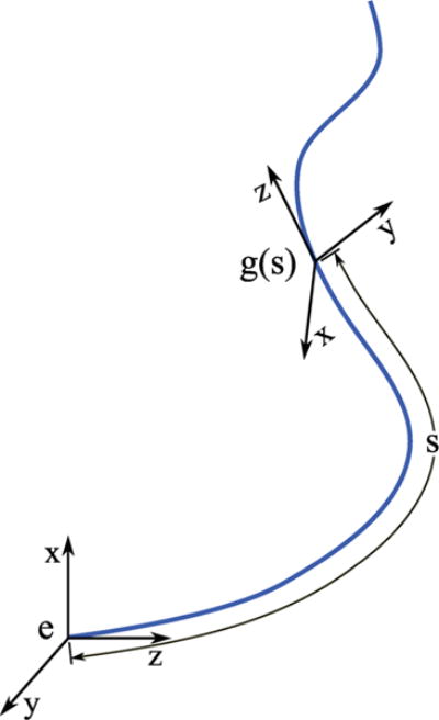
A parametrized set of reference frames defining an elastic filament.

Subject to Dirac delta initial conditions, f(g; 0) = δ(g) (throughout the text, δ will be used as both the Dirac delta and the Kronecker delta; the Kronecker delta will be indicated using subscript arguments such as δ_ab), the solution to the Fokker–Planck equation in eq 4 gives the distribution of relative positions and orientations at a point s along the sequence relative to the proximal end. The solution is a probability density function for each fixed value of s ∈ [0, L],

$$f(g;s)\ge 0\text{and}{\displaystyle {\int }_{G}f(g;s)\mathrm{d}g=1}$$ (6)

Here, the integral is over the group G with respect to the Haar measure dg. The Haar measure is used to provide a notion of consistent volume for the group allowing for a valid definition of an integral.²¹

The diffusion equation in eq 4 has been derived using several different analogies. First, the potential energy for a worm-like chain with flexibility in all six infinitesimal rigid-body motions is

$$\mathcal{V}=\frac{1}{2}{\displaystyle {\int }_0^L{[\xi -{\xi }_0]}^{T}K[\xi -{\xi }_0]\mathrm{d}s}$$

where K is the 6 × 6 stiffness matrix, L is the total length, and 0 ≤ s ≤ L. In several works,^17,22–24 a path integral approach was used viewing this total potential energy as the “kinetic energy” of a rigid body

$$\mathcal{T}=\frac{1}{2}{[\xi -{\xi }_0]}^{T}K[\xi -{\xi }_0]$$ (7)

(with K interpreted as a 6 × 6 inertial matrix) integrated along a trajectory. The relationship between D and K is

$$D\left(s\right)=\left(2k_{\mathrm{B}}T\right)K^{-1}\left(s\right)$$ (8)

where k_B is the Boltzmann constant, T is temperature in degrees Kelvin, and K is measured in units of k_BT. Therefore, the way to interpret eqs 4 and 8 is that diffusion is akin to flexibility, which is amplified by temperature.

Keeping with the analogy between s and time, the stochastic differential equation that is equivalent to eq 4 is

$${\left(g^{-1}\dot{g}\right)}^{\vee }\mathrm{d}s={\xi }_0\left(s\right)\mathrm{d}s+B\mathrm{d}\mathbf{w}$$ (9)

where $\mathrm{d}\mathbf{w}\in {ℝ}^6$ is a vector of uncorrelated unit-strength white noises and B is any matrix such that BB^T = D. For B = (2k_BT)^1/2K^−1/2, eq 9 can be written as

$$K\left(\xi -{\xi }_0\right)\mathrm{d}s=\sqrt{2k_{B}T}{K}^{1/2}\mathrm{d}\mathbf{w}$$ (10)

Equation 10 can be interpreted in such a way that K is neither the stiffness nor the inertia matrix. Rather, it is a damping matrix as if there were a six-dimensional dashpot connecting an infinitesimal part of the filament at curve parameter s, which is also acted on by thermal agitation with strength (2k_BT)^1/2K^1/2 consistent with the fluctuation–dissipation theorem.^25,26 When taking this point of view, $\mathcal{T}$ in eq 7 would not be the kinetic energy but rather this same quantity should be viewed as a Rayleigh dissipation function, and denoted as $ℛ$.

Two methods for solving eq 4 have been presented in the literature corresponding to two different scenarios. The first is for relatively short segments (i.e., those less than one persistence length). In this case, when using exponential coordinates, g = exp X, the approximation

$${{\stackrel{\sim }{E}}_{i}f(g_0(s)\circ {\mathrm{e}}^X)\approx \frac{\partial f}{\partial x_i}|}_{g_0(s)}$$

is valid because the probability density is concentrated around the baseline value. In this case, eq 4 reduces to a classical diffusion equation with a Gaussian solution of the form

$$f(g;s)=\frac{1}{\alpha ({\sum }_{g_0}(s))}\exp \{-\frac{1}{2}{[{(\log (g_0^{-1}(s)\circ g))}^{\vee }]}^T\cdot {[{\sum }_{g_0}(s)]}^{-1}{(\log (g_0^{-1}(s)\circ g))}^{\vee }\}$$ (11)

where

$${\sum }_{g_0}(s)={\displaystyle {\int }_0^s{\text{Ad}}^{-1}(g_0(\tau ))D(\tau ){({\text{Ad}}^{-1}(g_0(\tau )))}^T\mathrm{d}\tau }$$ (12)

and $\alpha ({\sum }_{g_0}(s))$ is a normalizing factor to make the function a pdf for each fixed value of s. For sufficiently concentrated distributions,

$$\alpha (\sum )\approx {(2\pi )}^3{|\sum |}^{1/2}$$ (13)

Alternatively, given f(g; s), the mean, g₀, and covariance, ${\sum }_{g_0}$, for any fixed value of s can be extracted so as to satisfy the conditions

$${\displaystyle {\int }_G{(\log (g_0^{-1}(s)\mathrm{o}g))}^{\vee }f(g;s)\mathrm{d}g}=\mathbf{0}$$ (14)

and

$${\displaystyle {\sum }_{g_0}(s)}={{\displaystyle {\int }_G(\log (g_0^{-1}(s)\circ g))}}^{\vee }{[{(\log (g_0^{-1}(s)\circ g))}^{\vee }]}^{T}f(g;s)\mathrm{d}g$$ (15)

For relatively long segments (from about half of a persistence length and longer), an alternative formulation based on the group Fourier transform is applicable. The only limitation on the filament lengths for which this model is applicable is that it is a phantom model, and does not account for excluded-volume effects. Therefore, in unconfined environments, this method (and the original governing equation, eq 4) is valid perhaps up to two or three persistence lengths. The group Fourier transform and corresponding inversion formula are written abstractly as

$$\begin{array}{l}\widehat{f}(\lambda )={\displaystyle {\int }_{G}f(g)U(g^{-1},\lambda )\mathrm{d}g\text{and}}\\ f(g)={\displaystyle {\int }_{\widehat{G}}\text{tr}[\widehat{f}(\lambda )U(g,\lambda )]\mathrm{d}(\lambda )}\end{array}$$ (16)

where λ is a “frequency” parameter drawn from the unitary dual of G, denoted as Ĝ, and {U(g, λ)|λ ∈ Ĝ} is a complete set of irreducible unitary representation matrices (the “hat” operator $(\widehat{·})$ was previously defined for elements of the Lie algebra; in this context, it will be used to represent the Fourier transform of a function).^16,21,27

The group Fourier transform has operational properties that are useful in solving eq 4. Namely, Fourier-space operator matrices, {W_i}, exist such that

$$\widehat{({\stackrel{\sim }{E}}_{i}f)}(\lambda )=W_i(\lambda )\widehat{f}(\lambda ,s)$$ (17)

This allows us to write

$$\begin{array}{l}\frac{\partial \widehat{f}(\lambda ,s)}{\partial s}=ℬ(s,\lambda )\widehat{f}(\lambda ,s)\text{where}\\ ℬ(s,\lambda )=\frac{1}{2}{\displaystyle \sum _{i,j=1}^6{D}_{ij}(s)W_i(\lambda )W_j(\lambda )}-{\displaystyle \sum _{k=1}^6({\xi }_0(s)\cdot {\mathbf{e}}_k)W_k(\lambda )}\end{array}$$ (18)

In the case when ξ₀(s) and D(s) are not sequence-dependent (e.g., pristine B-form DNA of homogeneous composition), $ℬ(s,\lambda )$ becomes independent of s. In this case, $ℬ(s,\lambda )={ℬ}_0(\lambda )$, and the Fourier-space solution simply becomes the matrix exponential $\widehat{f}(\lambda ,s)=\exp (s{ℬ}_0(\lambda ))$. In the more general case, the linear system of ordinary differential equations can be solved by numerical integration.^16,21,27

3.1. Bent DNA

One application of the elastic-filament model is in analyzing bent DNA. As shown in Figure 4, it is known that proteins bend DNA to activate or repress transcription;^28–34 DNA often forms loops or is wrapped around proteins,^7,35–42 and proteins scan (diffuse) along DNA to search for sites that are more flexible, or pre-bent.^30,43–47

Figure 4.

Five examples of DNA bending. Images generated from PDB data.^48–54

Moreover, many cancer drugs such as Cisplatin primarily target DNA and induce structural and mechanical changes like bending and cross-linking,⁵⁴ which can ultimately lead to apoptosis,^55,56 the desired outcome of cancer therapy. Cisplatin has a success rate of more than 90% against testicular and ovarian cancer but a low success rate for other cancers, such as lung cancer.⁵⁷ The underlying reason for these disparate success rates may be that DNA in different cancer cells responds differently to drug-induced DNA damage, such as DNA bends.^58–61 Cisplatin targets the major groove of DNA^62–64 and forms intrastrand biadducts between purine bases,^65,66 thus bending the major groove and subsequently opening up the minor groove. The major adduct is a 1,2-intrastrand adduct between adjacent guanine bases.⁶⁷ Despite the fact that this drug has been used for several decades, the structural changes induced by cisplatin in a DNA molecule, especially the local changes due to its interaction with a single molecule of cisplatin (e.g., bend angle, bend flexibility, binding geometry) are still debated, even though these properties may play a key role in how cellular proteins process this damage.^67,68 For example, the bend angle of a GG adduct in cisplatinated DNA, as determined by bulk experimental techniques and gel electrophoresis, NMR, and X-ray, ranges from 30 to 80°.^{54,62,69–72} However, recent high resolution X-ray data point to a bend angle between 35 and 40°.⁵⁴ In the discussion below, we compare the techniques derived for the elastic-filament model with experimental data.

Numerical and Experimental Results

Since stiffnesses are measured in terms of k_BT, it follows that, under the extreme condition T → 0, no diffusion would take place, and $f(g;0,s)\to \delta (g_0^{-1}(s)\mathrm{o}g)$. As T increases, these probability densities become less concentrated. For the biologically relevant case (T ≈ 300), eq 4 can be solved using the harmonic analysis approach summarized by eqs 16–18.^21,73,74 If we make the shorthand notation $f_{s_1,s_2}(g)=f(g;s_1,s_2)$, then it will always be the case for s₁ < s < s₂ that (the notations $f_{s_1,s_2}$ and f(s; s₁, s₂) are used interchangeably)

$$f_{s_1,s_2}(g)=(f_{s_1,s}\ast f_{s,s_2})(g)={\displaystyle {\int }_G{f}_{s_1,s}(h)f_{s,s_2}(h^{-1}\circ g)\mathrm{d}h}$$ (19)

This is the convolution of two position and orientation distributions. While eq 19 will always hold for semiflexible phantom chains, for the homogeneous rod, there is the additional convenient properties that

$$\begin{array}{l}f(g;s_1,s_2)=f(g;0,s_2-s_1)\text{and}\\ f(g;s_2,s_1)=f(g^{-1};s_1,s_2)\end{array}$$ (20)

The first of these says that for a uniform chain the position and orientation distribution only depend on the difference of arc length along the chain. The second provides a relationship between the position and orientation distribution for a uniform chain resulting from taking the frame at s₁ to be fixed at the identity and recording the poses visited by s₂, and the distribution of frames that results when s₂ is fixed at the identity. When eq 20 holds, we can use the shorthand f(g; s₁, s₂) = f(g; s₂ − s₁). Note that neither of these nor eq 19 will hold when excluded-volume interactions are taken into account, but our DNAs are short enough that excluded-volume effects are not important.

Since g describes fully the motion permissible in the group being considered, f(g; s) is a joint density in all rigid-body degrees of freedom and any of the usual quantities of interest in polymer theory can be extracted: end-to-end distance, ring closure probabilities, end-to-end orientation distributions, etc. When a bend is present, the distribution of end-to-end position and orientation can be formulated as a convolution of the form f(g; s₁)∗b(g)∗f(g; s₂), where b(g) describes the kind of bend/twist between two segments and convolution is defined as in eq 19. Candidates for the form of b(g), which are a product of delta functions in position and shifted delta functions in orientation, were given by Zhou and Chirikjian.⁷⁵ This convolution approach is particularly useful when coupled with the fact that for the group Fourier transform defined in eq 16

$$(\widehat{f_1\ast f_2})(\lambda )=\widehat{f_2}(\lambda )\widehat{f_1}(\lambda )$$ (21)

Figure 5 shows a series of position measurements along DNA conformations taken with an atomic force microscope (AFM) of an untreated and cisplatined 300 base pair DNA fragment. Conformations have been translocated in order that each proximal end has a common position and orientation. The DNA fragment had a single GG site in its center (G₁₅₀G₁₅₁) at which a GG intrastrand cisplatin cross-link was formed. The cisplatinated fragment had, thus, one central cisplatin-induced bend. The single GG sites in the DNA construct were selected because cisplatin has a high specificity of cross-linking GG sites in DNA.⁷⁶ The DNA substrate was treated with a 500-fold excess of cisplatin for 6 h and purified with a G-50 Sephadex spin column. Using inductively coupled plasma-mass spectrometry (ICP-MS), the platinum/DNA ratio was found to be 0.95, indicating nearly complete platination at the single GG site in the center of the fragment. The AFM images were obtained using deposition and imaging conditions in which the DNA molecules can equilibrate on the two-dimensional mica substrate.⁷⁷ In other words, the AFM-imaged DNA molecules behave like, and can be modeled as, worm-like chains constrained to a plane. The AFM-imaged molecules can then be compared to DNA molecules that were simulated with a range of different parameters, such as different persistence lengths (or diffusion constants) and different bend angles. Figure 6 shows simulated trajectories for unperturbed or “naked” DNA and for the same DNA that has a bend induced in the middle. The comparisons of the R/L distributions of the AFM-imaged DNA molecules and the simulated DNA molecules were done using the chi-squared test, the Ansari–Bradley test,⁷⁸ and the bootstrap method using Matlab statistical subroutines. Here R represents the end-to-end distance and L, the total arc length. Comparing the normalized end-to-end distance distributions of simulated and real DNA molecules, a persistence length of 45 nm was obtained for the unmodified DNA fragment. Comparing the distributions of cisplatinated molecules with the same methods and assuming a persistence length of 45 nm for the DNA arms, a cisplatin-induced bend angle in the range 30–44° was obtained, with the best fit giving a value of 36°.^79,80 This is in very good agreement with the values obtained from gel electrophoresis and X-ray experiments^{54,69,71,72,81} but disagrees with other published values.^70,82

Figure 5.

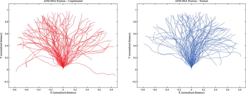
Two ensembles of DNA conformations as measured using an AFM: (left) cisplatinated DNA; (right) naked DNA.

Figure 6.

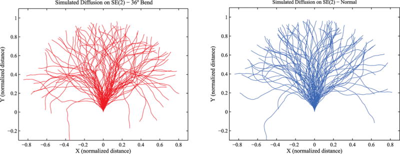
Two simulated ensembles of stochastic trajectories: (left) with a 36° bend; (right) without a bend.

This model is confined to SE(2), the planar motion group; however, most of what has been discussed to this point with regards to SE(3) still holds for SE(2), except for the explicit forms of the elements of SE(2) and its associated Lie algebra, se(2). These are naturally different, since elements of SE(2) only have three degrees of freedom (as opposed to the six for SE(3)). These elements of SE(2) can be represented with homogeneous matrices of the form

$$g(\theta ,r,\varphi )=\left(\begin{array}{lll}\cos (\theta )\hfill & -\sin \theta \hfill & r\cos (\varphi )\hfill \\ \sin (\theta )\hfill & \cos (\theta )\hfill & r\sin (\varphi )\hfill \\ 0\hfill & 0\hfill & 1\hfill \end{array}\right)$$ (22)

using polar coordinates. Similar to eq 2, the infinitesimal generators of SE(2) are

$$E_1=\left(\begin{array}{lll}0\hfill & -1\hfill & 0\hfill \\ 1\hfill & 0\hfill & 0\hfill \\ 0\hfill & 0\hfill & 0\hfill \end{array}\right);E_2=\left(\begin{array}{lll}0\hfill & 0\hfill & 1\hfill \\ 0\hfill & 0\hfill & 0\hfill \\ 0\hfill & 0\hfill & 0\hfill \end{array}\right);E_3=\left(\begin{array}{lll}0\hfill & 0\hfill & 0\hfill \\ 0\hfill & 0\hfill & 1\hfill \\ 0\hfill & 0\hfill & 0\hfill \end{array}\right)$$

We can simulate a model of the worm-like chain to obtain statistics that can be compared with the AFM measurements. For example, the simulated strands in Figure 6 can be generated using a version of eq 9 of the form

$$\left(\begin{array}{l}{\xi }_1\\ {\xi }_2\\ {\xi }_3\end{array}\right)\mathrm{d}s=\left(\begin{array}{l}0\\ 0\\ 1\end{array}\right)\mathrm{d}s+\left(\begin{array}{l}\sqrt{2\eta }\\ 0\\ 0\end{array}\right)\mathrm{d}{w}_1$$ (23)

Thus, the unperturbed path would have a constant “velocity” in the y direction. If we then look at the sampled means and covariances of the simulated and experimental data as defined in eqs 14 and 15 where the integrals are replaced with summations over the sampled values, we can determine whether or not our model accurately reflects the underlying phenomenon. The orientation of the distal end of the experimental data was approximated using the tanget of the curve at the end. For the data shown in Figures 5 and 6 where η = 0.7, the means of the four data sets were very similar. However, we can look at the sample covariances for the naked DNA

$$\begin{array}{l}{\sum }_{\text{AFM}}^{\text{Naked}}=\left(\begin{array}{lll}0.323\hfill & 0.032\hfill & -0.587\hfill \\ 0.032\hfill & 0.057\hfill & -0.073\hfill \\ -0.587\hfill & -0.073\hfill & 1.384\hfill \end{array}\right)\text{and}\\ {\sum }_{\text{Sim}}^{\text{Naked}}=\left(\begin{array}{lll}0.393\hfill & 0.012\hfill & -0.595\hfill \\ 0.012\hfill & 0.046\hfill & -0.018\hfill \\ -0.595\hfill & -0.018\hfill & 1.217\hfill \end{array}\right)\end{array}$$

and the bent DNA

$$\begin{array}{l}{\sum }_{\text{AFM}}^{\text{Bent}}=\left(\begin{array}{lll}0.480\hfill & -0.058\hfill & -0.829\hfill \\ -0.058\hfill & 0.076\hfill & 0.132\hfill \\ -0.829\hfill & 0.132\hfill & 1.781\hfill \end{array}\right)\text{and}\\ {\sum }_{\text{Sim}}^{\text{Bent}}=\left(\begin{array}{lll}0.593\hfill & -0.037\hfill & -0.973\hfill \\ -0.037\hfill & 0.062\hfill & 0.054\hfill \\ -0.973\hfill & 0.054\hfill & 1.853\hfill \end{array}\right)\end{array}$$

These numbers show that the simulated and measured data sets for naked DNA (or bent DNA) are more similar to each other than the two simulated (or measured) data sets are to each other. This can be expressed quantitatively by looking at the Frobenius norm of the difference between these matrices normalized as shown below. These normalized differences are calculated to be

$$\begin{array}{l}\frac{\Vert {\sum }_{\text{AFM}}^{\text{Naked}}-{\sum }_{\text{Sim}}^{\text{Naked}}\Vert }{\Vert {\sum }_{\text{AFM}}^{\text{Naked}}\Vert }=0.1210,\\ \frac{\Vert {\sum }_{\text{AFM}}^{\text{Bent}}-{\sum }_{\text{Sim}}^{\text{Bent}}\Vert }{\Vert {\sum }_{\text{AFM}}^{\text{Bent}}\Vert }=0.1229,\\ \frac{\Vert {\sum }_{\text{AFM}}^{\text{Naked}}-{\sum }_{\text{AFM}}^{\text{Bent}}\Vert }{\Vert {\sum }_{\text{AFM}}^{\text{Naked}}\Vert }=0.3828,\text{and}\\ \frac{\Vert {\sum }_{\text{Sim}}^{\text{Naked}}-{\sum }_{\text{Sim}}^{\text{Bent}}\Vert }{\Vert {\sum }_{\text{Sim}}^{\text{Naked}}\Vert }=0.5637,\end{array}$$

In addition to numerically simulating trajectories, the probability density function on the motion group can be obtained using Fourier techniques. Similar to the approach taken in previous work on SE(3),¹⁷ a probability density function on the motion group SE(2) can be defined to describe the ensemble of conformations of an elastic filament. For the examples presented (contour plots shown in Figure 7), the following was used

$$\frac{\partial f}{\partial s}=(\eta {({\stackrel{\sim }{E}}_1)}^2+{\stackrel{\sim }{E}}_3)f$$ (24)

This is equivalent to the model given in eq 23. Using properties of the group Fourier transform from eqs 16 and 17, we can write

$$\frac{\mathrm{d}\widehat{f}}{\mathrm{d}s}=(\eta {(W_1(\lambda ))}^2+W_3(\lambda ))\widehat{f}$$ (25)

where W_i(λ)’s are found using

$$W_i(\lambda )={\left(\frac{\mathrm{d}}{\mathrm{d}t}U(\exp (s{E}_i),\lambda )\right)|}_{s=0}$$

These matrices, which are infinite-dimensional, can be shown to be

$${[W_1]}_{mk}(\lambda )=-jk{\delta }_{m,k}$$ (26)

$${[W_2]}_{mk}(\lambda )=\frac{j\lambda }{2}[{\delta }_{k,m+1}+{\delta }_{n,m-1}]$$ (27)

$${[W_3]}_{mk}(\lambda )=\frac{\lambda }{2}[{\delta }_{k,m-1}-{\delta }_{k,m+1}]$$ (28)

when the irreducible representation matrices, U(g, λ), used for SE(2) are

$$U_{mk}(g(\theta ,r,\varphi ),\lambda )=j^{k-m}{\mathrm{e}}^{-j[k\theta +(m-k)\varphi ]}{J}_{k-m}(\lambda r)$$

Here J_p(·) is the pth-order Bessel function, j = (−1)^1/2, and matrices are indexed such that m, k ∈ ℤ. It should then be clear that

$$\widehat{f}(\lambda ;s)=\exp (s(\eta {(W_1(\lambda ))}^2+W_3(\lambda )))$$ (29)

and, using the inverse Fourier transform from eq 16,

$$f(g;s)={\displaystyle \sum _{m,k\in \mathbb{Z}}{\displaystyle {\int }_0^{\infty }{\widehat{f}}_{mk}}}(\lambda ;s)U_{km}(g,\lambda )\lambda \text{ d}\lambda$$ (30)

Figure 7.

Distribution of the distal end position of the model relative to the proximal end: (left) with a 36° bend; (right) without a bend.

If we assume a static bend of the form²¹

$$b({\theta }_0)=\frac{\delta (r)}{r}\delta (\theta -{\theta }_0)$$ (31)

where δ(·) is the Dirac delta and θ₀ is the bend angle, we can use eqs 21, 29, and 30 to determine the pdf of two lengths of elastic filament connected by a static bend. Sample contour plots for such distributions are shown in Figure 7 for unit length and η = 0.7. In the bent example, the 36° bend occurs at the midpoint of the filament. Though the largest disparities may occur in the orientation, these contour plots have been marginalized over θ so that just the position remains. This was done because orientation is not as easily measured experimentally.

For the numerical integration, the infinite dimensional Fourier-space operator matrices, {W_i}, were truncated to 29 × 29 before exponentiation. Further truncation to 15 × 15 was performed prior to applying the Fourier inversion formula (eq 30) which was numerically integrated from λ = 0 to 100 using a step size of 0.1.

The contour plots in Figure 7 help to illustrate the differences inherent in the underlying distributions for bent and straight DNA. The broader shape and less severe peak in the contour plot associated with the bent case highlights the “smearing” effect that the addition of a bend has. This effect is more pronounced as η increases.

4. BI-ROD MODEL

In the bi-rod model due to Moakher and Maddocks,⁸³ double-helical DNA is considered to be two intertwined helical elastic rods connected with elastic contacts. On short length scales, this has different properties than the single elastic filament, whereas, on long length scales, it must converge to the single filament model, which has been verified experimentally.

Consider a bi-rod consisting of two elastic filaments described as trajectories l(s),r(s) ∈ G for s ∈ [0,L]. Here we can think of these as a “left” and “right” filament, though they are intertwined and continually reverse order as s increases. In the referential configuration of standard B-form double-helical DNA, the backbone is given by

$$g_0(s)=\left(\begin{array}{ll}{R}_3(2\pi ns/L)\hfill & s{\mathbf{e}}_3\hfill \\ {\mathbf{0}}^T\hfill & 1\hfill \end{array}\right)=\text{screw}({\mathbf{e}}_3,2\pi ns/L,s)$$ (32)

where L/n is the helical repeat length (i.e., the helix makes n revolutions over a length L) and R₃(θ) is the rotation matrix describing counterclockwise rotation around the e₃-axis. The referential shapes of the two elastic filaments in the bi-rod are helical and are defined by

$$r_0(s)=g_0(s)\circ {\delta }_0\text{and}{l}_0(s)=g_0(s)\circ {\delta }_0^{-1}$$

for

$${\delta }_0=\text{trans}\left(\frac{1}{2}w{\mathbf{e}}_1\right)$$ (33)

where w is the distance between the centerlines of each filament in the bi-rod (here δ₀ ∈ G = SE(3) is a small rigid-body motion, and is unrelated to the Kronecker and Dirac delta functions used earlier).

Small deviations from this baseline shape can be described as

$$g(s)=g_0(s)\circ \exp (X_g)\text{and}\delta (s)={\delta }_0\circ \exp (X_{\delta })$$

where $\exp (X_{g,\delta })\approx {\mathbb{I}}_4+X_{g,\delta }$. The left and right filaments can then be written as

$$r(s)=g(s)\circ \delta (s)\text{and}l(s)=g(s)\circ {\delta }^{-1}(s)$$

Figure 8 illustrates the relationship between the left and right frames.

Figure 8.

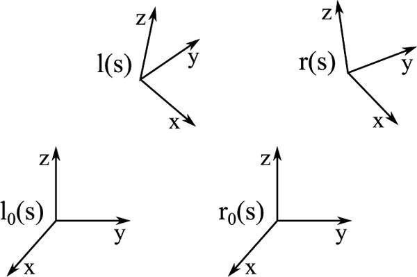
The relationship between reference frames in the bi-rod model.

We now focus on the derivation of f(r, l; s) or alternatively f(g, δ; s), with the ultimate goal of determining D(s) or K(s). The probability density f(r, l; s) is one on the space G × G, which as a group is the direct product of G with itself. As a result, the adjoint matrices in eq 3 extend to G × G as direct sums. For example, Ad(r, l) = Ad(r) ⊕ Ad(l). Similar expressions hold for ad(·), exp(·), and log(·).

The bi-rod version of eq 10 (again with s taking the place of time) can be derived by starting with the Rayleigh dissipation function

$$ℛ=\frac{1}{2}{({\xi }_r-{\xi }_{r_0})}^T{W}_r({\xi }_r-{\xi }_{r_0})+\frac{1}{2}{({\xi }_l-{\xi }_{l_0})}^T{W}_l({\xi }_r-{\xi }_{l_0})$$

and the potential energy

$$\mathcal{V}=\frac{1}{2}{\{\log {({[l^{-1}\circ r]}^{-1}\circ l_0^{-1}\circ r_0)}^{\vee }\}}^{T}W\log {({[l^{-1}\circ r]}^{-1}\circ l_0^{-1}\circ r_0)}^{\vee }$$

Here W_r and W_l are symmetric weighting matrices for the right and left rods. As mentioned before in the context of worm-like chains, in some analogies, these matrices are stiffness matrices and in other analogies they are viewed as inertia matrices. At present, they are viewed as damping matrices. For the potential energy, W is a symmetric matrix that defines the spring force between the two rods. The resulting coordinate-free version of Lagrange’s equations of motion with damping and external forcing, but without inertial terms, will be of the form

$$\frac{\partial ℛ}{\partial {\xi }_l}+{\stackrel{\mathbf{\sim }}{\mathbf{E}}}_l\mathcal{V}={\mathbf{n}}_l(s)\text{and}\frac{\partial ℛ}{\partial {\xi }_r}+{\stackrel{\mathbf{\sim }}{\mathbf{E}}}_r\mathcal{V}={\mathbf{n}}_r(s)$$ (34)

where the total noise vector is related to a vector of uncorrelated unit-strength Wiener processes as

$$\mathbf{n}(s)\mathrm{d}s=\left(\begin{array}{l}{\mathbf{n}}_l(s)\\ {\mathbf{n}}_r(s)\end{array}\right)\mathrm{d}s=\sqrt{2k_{B}T{Z}^{\prime }}\mathrm{d}\mathbf{w}$$

If, in analogy with eq 10 the diffusion and damping satisfy detailed balance conditions, then the coupling matrix Z′ is

$$Z^{\prime }={\left(\begin{array}{ll}{W}_l\hfill & O\hfill \\ O\hfill & W_r\hfill \end{array}\right)}^{1/2}$$

The governing equations (eq 34) can be written explicitly for the case when $X_g^{\vee }$ and $X_{\delta }^{\vee }$ (and their derivatives with respect to s, ${\dot{X}}_g^{\vee }$ and ${\dot{X}}_{\delta }^{\vee }$) have small magnitudes. In this case, neglecting all but the linear terms in $X_g^{\vee }$ and $X_{\delta }^{\vee }$ and their derivatives, the following approximations can be made

$$\begin{array}{l}\log {({[l^{-1}r]}^{-1}{l}_0^{-1}{r}_0)}^{\vee }\approx -\text{Ad}({\delta }_0^{-1})X_{\delta }^{\vee }-X_{\delta }^{\vee }\\ {\stackrel{\mathbf{\sim }}{\mathbf{E}}}_l\mathcal{V}\approx -{\text{Ad}}^T({\delta }_0^{-1}{\delta }_0^{-1})W(\mathbb{I}+\text{Ad}({\delta }_0^{-1}))X_{\delta }^{\vee }\\ {\stackrel{\mathbf{\sim }}{\mathbf{E}}}_r\mathcal{V}\approx W(\mathbb{I}+\text{Ad}({\delta }_0^{-1}))X_{\delta }^{\vee }\\ \frac{\partial ℛ}{\partial {\xi }_l}\approx W_l\text{Ad}({\delta }_0)(\text{ad}(g_0^{-1}{\dot{g}}_0)X_g^{\vee }-\text{ad}(g_0^{-1}{\dot{g}}_0)X_{\delta }^{\vee }+{\dot{X}}_g^{\vee })\\ \frac{\partial ℛ}{\partial {\xi }_r}\approx W_r(\text{ad}({\delta }_0^{-1}{g}_0^{-1}{\dot{g}}_0{\delta }_0)X_{\delta }^{\vee }+\text{Ad}({\delta }_0^{-1})\text{ad}(g_0^{-1}{\dot{g}}_0)X_g^{\vee }+\text{Ad}({\delta }_0^{-1}){\dot{X}}_g^{\vee }+{\dot{X}}_{\delta }^{\vee })\end{array}$$

If we define

$$\mathbf{x}=\left(\begin{array}{l}{X}_g^{\vee }\\ X_{\delta }^{\vee }\end{array}\right)$$

the stochastic differential equations describing the bi-rod can be written in the form

$$\mathrm{d}\mathbf{x}=-Q\mathbf{x}\mathrm{d}t+Z\mathrm{d}\mathbf{w}$$ (35)

where

$$\begin{array}{l}Q=H^{-1}\left(\begin{array}{ll}\text{Ad}({\delta }_0^{-1})\text{ad}(g_0^{-1}{\dot{g}}_0)\hfill & \text{ad}({\delta }_0^{-1}{g}_0^{-1}{\dot{g}}_0{\delta }_0)+W_r^{-1}W(\mathbb{I}+\text{Ad}({\delta }_0^{-1}))\hfill \\ \text{ad}(g_0^{-1}{\dot{g}}_0)\hfill & -\text{ad}(g_0^{-1}{\dot{g}}_0)-\text{Ad}({\delta }_0^{-1})\cdot W_l^{-1}{\text{Ad}}^T({\delta }_0^{-1}{\delta }_0^{-1})\cdot W(\mathbb{I}+\text{Ad}({\delta }_0^{-1}))\hfill \end{array}\right)\\ Z=\sqrt{2k_{B}T}{H}^{-1}\left(\begin{array}{ll}{W}_r^{-1/2}\hfill & \mathbf{0}\hfill \\ \mathbf{0}\hfill & \text{Ad}({\delta }_0^{-1})W_l^{-1/2}\hfill \end{array}\right)\end{array}$$

and

$$H=\left(\begin{array}{ll}\text{Ad}({\delta }_0^{-1})\hfill & \mathbb{I}\hfill \\ \mathbb{I}\hfill & -\mathbb{I}\hfill \end{array}\right)$$

These equations define a degenerate Ornstein–Uhlenbeck process. It is degenerate because the 12 × 12 matrix Q has rank ten with six eigenvalues with a zero real part. In other words, six degrees of freedom have elastic constraints on them from contact between the bi-rods, and six of the degrees of freedom feel only Brownian forcing.

Our goal is to obtain the corresponding probability density f(g, δ; s) and marginalize over δ. This will allow for the reconciliation of the bi-rod model with the elastic-filament model given in section 3. Using the fact that eq 35 is an Ornstein–Uhlenbeck process allows us to say that f(g, δ; s) is Gaussian. Details of the techniques used to demonstrate this can be found in the Supporting Information.

When Q has distinct eigenvalues, it can be expanded using the spectral decomposition as

$$Q=U\mathrm{\Lambda }{V}^T={\displaystyle \sum _{i=1}^n{\lambda }_i{\mathbf{u}}_i{\mathbf{v}}_i^T}$$

Here U = [u₁,…, u_n] and V = [v₁,…, v_n] are matrices such that the columns satisfy the following equations:

$$Q{\mathbf{u}}_i={\lambda }_i{\mathbf{u}}_i{Q}^T{\mathbf{v}}_i={\lambda }_i{\mathbf{v}}_i$$

If Q is independent of s then, as detailed in the Supporting Information, the derivative of the covariance Σ with respect to s is given by

$$\dot{\sum }(s)={\displaystyle \sum _{i,j}\exp (-({\lambda }_i+{\lambda }_j)s)({\mathbf{v}}_i^{T}Z{Z}^T{\mathbf{v}}_j)}{\mathbf{u}}_i{\mathbf{u}}_j^T$$ (36)

Since we know that f(g, δ; s) is Gaussian, we can write

$$f(g,\delta ;s)=\frac{1}{\alpha (\sum (s))}\exp \left(-\frac{1}{2}{\mathbf{x}}^T\sum {(s)}^{-1}\mathbf{x}\right)$$ (37)

for an appropriate normalizing function α(Σ(s)) and

$$\sum (s)=\left(\begin{array}{ll}{\sum }_{g_0}(s)\hfill & {\sum }_{g_0,{\delta }_0}(s)\hfill \\ {\sum }_{g_0,{\delta }_0}^T(s)\hfill & {\sum }_{{\delta }_0}(s)\hfill \end{array}\right)$$

Marginalizing over $X_{\delta }^{\vee }$ yields a probability density in $X_g^{\vee }$ that is also Gaussian with zero mean and covariance ${\sum }_{g_0}(s)$. We can relate this to the equivalent stiffness matrix defined in the context of the single elastic filament. Once ${\sum }_{g_0}(s)$ has been computed, the effective or equivalent diffusion matrix for the worm-like chain can be extracted by inverting eq 12 as

$$D(s)=\text{Ad}(g_0(s)){\dot{\sum }}_{g_0}(s){\text{Ad}}^T(g_0(s))$$

where ${\dot{\sum }}_{g_0}(s)=(\text{d/ds}){\sum }_{g_0}(s)$. The effective stiffness can then be computed using eq 8. This effective stiffness was determined as a function of s for B-form DNA with a width w of 2 nm and a pitch L/n of 3.4 nm. The damping and spring contact matrices used were

$$W_r=W_l=\left(\begin{array}{ll}{c}_1{\mathbb{I}}_3\hfill & O\hfill \\ O\hfill & c_2{\mathbb{I}}_3\hfill \end{array}\right)\text{and}W=\left(\begin{array}{ll}{c}_3{\mathbb{I}}_3\hfill & O\hfill \\ O\hfill & c_4{\mathbb{I}}_3\hfill \end{array}\right)$$

Figures 9 and 10 demonstrate how these effective stiffnesses converge to stable values as s increases. Figure 9 illustrates how individual elements of the effective stiffness matrix converge to steady-state values. In Figure 10, the Frobenius norm of the difference between the equivalent stiffness matrix at s and the steady-state equivalent stiffness matrix is plotted as a function of s. These plots also demonstrate that, although the damping and spring contact matrices for the bi-rod model are constant with respect to s, the effective or equivalent stiffness varies as a function of s. However, since the effective stiffness converges to a steady-state value as s increases, the effective stiffness can be taken as a constant for sufficiently long rods. While the speed of convergence is a function of the parameter values, these examples provide numerical validation that the bi-rod and elastic-filament models indeed do converge as s (and thus length) increases.

Figure 9.

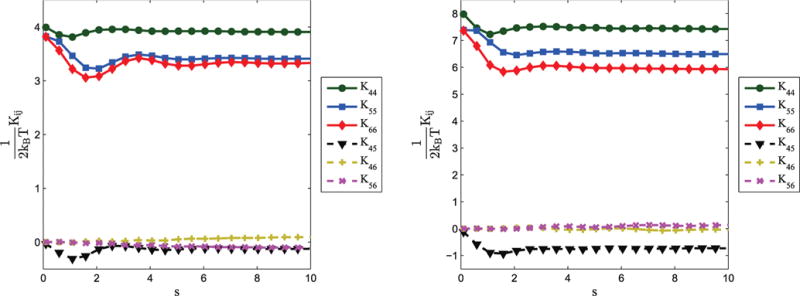
Examples of how the effective stiffness matrix, K(s), varies for the values associated with rotation. Results are shown for two different sets of parameters: (left) c₁ = 10, c₂ = 2, c₃ = 2, c₄ = 1; (right) c₁ = 10, c₂ = 4, c₃ = 5, c₃ = ¹/₂.

Figure 10.

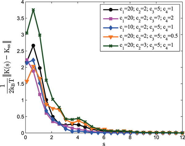
Examples of how the effective stiffness of the bi-rod model, K(s), differs from its steady-state value, K_ss, for various values of W_l/r and W. Here the Frobenius norm is used.

5. RIGID-BASE-PAIR MODELS

The rigid-base-pair model uses a rigid body to represent each base pair in a strand of DNA or RNA. These rigid bodies are attached to adjacent base pairs through elastic constraints. As such, the rigid-base-pair model can be viewed as a discretized version of the single-elastic-filament model by assigning reference frames to each DNA or RNA base pair.

A number of approaches for attaching representative reference frames to base pairs have been used in the literature and in programs used to describe three-dimensional arrangements of DNA and RNA structures. A quantitative description of some of the discrepancies between the different approaches was presented by Lu et al.⁸⁴

We will use the method in which the reference frames are positioned so that complementary bases form an ideal, planar Watson–Crick base-pair in the undistorted reference state with values of hydrogen bond donor–acceptor distances, C1′⋯C1′ virtual lengths, and purine N9–C1′⋯C1′ and pyrimidine N1–C1′⋯C1′ virtual angles consistent with those found in the crystal structures of small molecules.

Given this base frame assignment, we can say that, relative to the previous base pair, the kth base pair has a distribution f_k(g) with mean g_k that satisfies

$$\mathbf{0}={\displaystyle {\int }_G{\log }^{\vee }(g_k^{-1}\circ g)f_k(g)\mathrm{d}g}$$ (38)

and covariance Σ_k defined by

$${\sum }_k={\displaystyle {\int }_G{\log }^{\vee }(g_k^{-1}\circ g){[{\log }^{\vee }(g_k^{-1}\circ g)]}^T{f}_k(g)\mathrm{d}g}$$ (39)

Then, for two base pairs with distributions f₁(g) and f₂(g), means g₁ and g₂, and covariances Σ₁ and Σ₂, the resulting distribution of stacking the two base pairs on top of each other can be represented as the convolution of the two distributions with

$$f_{1\ast 2}(g)=(f_1\ast f_2)(g)={\displaystyle {\int }_G{f}_1(h)f_2(h^{-1}\circ g)\mathrm{d}h}$$ (40)

This new distribution will have mean g_1*2 and covariance Σ_1*2. An exact analytical solution for g_1*2 and Σ_1*2 is not known in general for Lie groups; however, so-called “first-order” and “second-order” approximations do exist for these quantities in SE(3). Such approximations were first introduced by Wang and Chirikjian in the context of serial robotic manipulators.^85–88 A similar concept was later applied to DNA by Becker and Everaers.^89,90

A first-order approximation will be presented here for the convolution of two distributions. Using this recursively allows one to determine the mean and covariance of N base pairs. As will be shown in section 5.2, if N or the individual covariances are sufficiently large, the resulting distribution, f_1*2*⋯*N, is described well with a Gaussian of the form

$$f_{1\ast 2\ast \cdots \ast N}(g)=\frac{1}{\alpha ({\sum }_{1\ast 2\ast \cdots \ast N})}\exp \left\{-\frac{1}{2}{\mathbf{x}}^T{[{\sum }_{1\ast 2\ast \cdots \ast N}]}^{-1}\mathbf{x}\right\}$$ (41)

for

$$\mathbf{x}={(\log (g_{1\ast 2\ast \cdots \ast N}^{-1}\circ g))}^{\vee }$$ (42)

where α(Σ_1*2*⋯*N) is a normalizing factor as described in eq 13.

In the first-order theory of covariance propagation, we make the approximation $\log (g_2^{-1}\circ g_1)=X_1-X_2$ or equivalently ${\left[\log (g_2^{-1}\circ g_1)\right]}^{\vee }={\mathbf{x}}_1-{\mathbf{x}}_2$, where g_i = exp(X_i) are elements of SE(3). This converts the convolution integral over the group into one over the Lie algebra se(3), which can be associated with ℝ⁶ via the ⋁ operator. The results are propagation formulas that produce the mean and covariance of the convolution of two functions in SE(3) from the means and covariances of the two original distributions and the relative motion of the mean of the second distribution relative to the first.^86,87,89 The mean and covariance of this approximation are

$$g_{1\ast 2}=g_1\circ g_2$$ (43)

and

$${\sum }_{1\ast 2}=\text{Ad}(g_2^{-1}){\sum }_1{\text{Ad}}^T(g_2^{-1})+{\sum }_2$$ (44)

These formulas can be used to “piece together” serially connected distributions (each describing small motions) into a distribution that describes the overall distribution of the distal end of a semiflexible chain relative to its base. Using the fact that the adjoint is a homomorphism (i.e., Ad(g₁◦g₂) = Ad(g₁)Ad(g₂) and Ad(g⁻¹) = Ad⁻¹(g)), the covariance propagation formula generalizes to the concatenation of N reference frames with concentrated distributions as

$${\sum }_{1\ast 2\ast \cdots \ast N}={\displaystyle \sum _{k=1}^N{\text{Ad}}^{-1}(g_{k+1}\circ \cdots \circ g_N){\sum }_k{\text{Ad}}^{-T}(g_{k+1}\circ \cdots \circ g_N)}$$ (45)

To simplify the notation in the subsequent sections, the covariance propagation is simply denoted as

$${\sum }_{1,N}={\displaystyle \sum _{k=1}^N{\text{Ad}}_{g(k)}^{-1}{\sum }_k{\text{Ad}}_{g(k)}^{-T}}$$ (46)

It should be noted that the first-order covariance propagation detailed in eq 46 works relatively well for convolving distributions that are relatively concentrated (i.e., small values of ‖Σ_k‖). This is typically the case for DNA and RNA, as they are relatively stiff. However, in cases where this assumption breaks down, a second-order approximation can be used. The details of this second-order propagation can be found in the literature.⁸⁸

5.1. Inverse Propagation of Covariance

The recursive propagation scheme presented in eqs 44 and 46 assumes that values for Σ_k’s are known. This may not always be the case. However, if Σ_1,N = Σ_data is known or can be obtained through dynamics simulations, then estimates of Σ_k can be obtained. These estimates assume that Σ_k is not dependent on k.

Since covariance matrices have a defined form, they can be represented as

$$\sum ={\displaystyle \sum _{i=1}^P{\sigma }_i{S}_i}$$ (47)

where Si is the ith basis element for the set of all possible symmetric 6 × 6 matrices and P is the number of basis elements. Since a symmetric n × n matrix is defined by n(n + 1)/2 independent entries, there are 21 independent entries in an SE(3) covariance matrix. Since the choice of the basis {S_i} is not unique, a natural choice for S_i is a matrix of the form ${\mathbf{e}}_j{\mathbf{e}}_j^T$ for the diagonal elements and ${\mathbf{e}}_j{\mathbf{e}}_k^T+{\mathbf{e}}_k{\mathbf{e}}_j^T$ for the off-diagonal elements, where e_j are the natural basis vectors for ℝ⁶.

Expanding Σ_data and Σ_k from eq 46 in this way so that ${\sum }_{\text{data}}={\displaystyle {\sum }_{i=1}^P{\sigma }_i^{\text{data}}{S}_i}$ and ${\sum }_k={\displaystyle {\sum }_{i=1}^P{\sigma }_i^k{S}_i}$, we have

$${\displaystyle \sum _{i=1}^P{\sigma }_i^{\text{data}}{S}_i={\displaystyle \sum _{k=1}^N{\text{Ad}}_{g(k)}^{-1}({\displaystyle \sum _{i=1}^P{\sigma }_i^k{S}_i}){\mathrm{Ad}}_{g(k)}^{-T}}}$$ (48)

$$={\displaystyle \sum _{i=1}^P{\sigma }_i^k({\displaystyle \sum _{k=1}^N{\text{Ad}}_{g(k)}^{-1}(S_i){\mathrm{Ad}}_{g(k)}^{-T}})}$$ (49)

The symmetric matrix ${\sum }_{k=1}^N{\text{Ad}}_{g(k)}^{-1}(S_i){\text{Ad}}_{g(k)}^{-T}$ can be expressed as

$${\displaystyle \sum _{k=1}^N{\text{Ad}}_{g(k)}^{-1}}(S_i){\mathrm{Ad}}_{g(k)}^{-T}={\displaystyle \sum _{m=1}^P{\psi }_{im}{S}_m}$$ (50)

and

$$\begin{array}{l}{\displaystyle \sum _{i=1}^P{\sigma }_i^{\text{data}}{S}_i}={\displaystyle \sum _{i=1}^P{\sigma }_i^k{\displaystyle \sum _{m=1}^P{\psi }_{\mathit{im}}{S}_m}}\\ ={\displaystyle \sum _{m=1}^P{\sigma }_m^k{\displaystyle \sum _{i=1}^P{\psi }_{\mathit{mi}}{S}_i}}\\ ={\displaystyle \sum _{m=1}^P{\displaystyle \sum _{i=1}^P{\psi }_{\mathit{mi}}{\sigma }_m^k{S}_i}}\end{array}$$

Thus, it is clear that

$${\displaystyle \sum _{i=1}^P({\sigma }_i^{\text{data}}}-{\displaystyle \sum _{m=1}^P{\psi }_{mi}{\sigma }_m^k)S_i=0}$$ (51)

and

$${\sigma }_i^{\text{data}}={\displaystyle \sum _{m=1}^P{\psi }_{mi}{\sigma }_m^k}$$

for i = 1, 2, …, P. Since S_i is a basis element, the resulting relation simplifies to the matrix expression

$${\sigma }^{\text{data}}={\mathbf{\Psi }}^T{\sigma }^k$$ (52)

where

$$\begin{array}{c}{\sigma }^{\text{data}}={[{\sigma }_1^{\text{data}},{\sigma }_2^{\text{data}},\dots ,{\sigma }_P^{\text{data}}]}^T\\ {\sigma }^k={[{\sigma }_1^k,{\sigma }_2^k,\dots ,{\sigma }_P^k]}^T\end{array}$$

Then, if Ψ^T is invertible, we can solve for σ^k and then compute the helix stiffness parameters from $(1/2k_{B}T)K={\sum }_k^{-1}$. This problem is similar to the estimation of model parameters for steerable needles described by Park et al.⁹¹

5.2. Statistics of Molecular Dynamics Simulations

Molecular dynamics simulations have been used to explore both rigid-base and rigid-base-pair models of DNA.^92,93 In this work, to determine whether the model proposed in eq 41 is valid, molecular dynamics simulations were performed on standard A-RNA helices which are stiffer than B-DNA. These models were built using Insight II (Accelrys, San Diego, CA, USA). Each helix consists of 14 base pairs with different compositions. The simulations were done for 16 ns using Amber 8.0.⁹⁴ The simulations used the ff99 Cornell force field for RNA,⁹⁵ which has proven to be a reliable force field for nucleic acids and the Amber molecular dynamics software. For the discussions below, we will say that simulations were simulated for n_t time steps and that the rigid-body transformation between the distal base pairs (g₁ and g_N) at time step i is $g^i=g_1^{-1}{g}_N$ for i = 1, 2,…, n_t. The mean of all gⁱ’s will be noted as g_μ.

Time Series Analysis and Stationarity of Molecular Dynamics Simulation

To analyze the stationarity of the helix during the molecular dynamics simulation, the transformation matrix g_μ is used to compute the cross-covariance matrices. For the Lie group of rigid-body motions, the cross-covariance matrices at lag l are computed as

$${\mathrm{\Gamma }}_{n_t}(l)=\frac{1}{n_t}{\displaystyle \sum _{i=1}^{n_t}[\log {(g_{\mu }^{-1}\circ g_i)}^{\vee }]{[\log {(g_{\mu }^{-1}\circ g_{i+l})}^{\vee }]}^T]}$$

Frequently, autocorrelation plots are used to check randomness in a data set. Randomness can be ascertained by computing autocorrelations for data values at varying time lags. Random data sets have autocorrelations near zero for the time-lag separations. Conversely, if the data set is not random, then one or more of the autocorrelations will be significantly nonzero. To generate an autocorrelation plot of the cross-covariance elements, we first calculated the singular values of the cross-covariance matrix. We then plotted the singular values against several different values for the lag, with the maximum lag equal to n_t/4. Autocorrelation plots are shown in Figures 11 and 12. For each sequence, g_i and g_μ represent the relative transformation from base-pair 3 to 12. The first and last two base-pairs were excluded from the calculations to prevent the inclusion of artifacts that might be due to end-effects during simulation.

Figure 11.

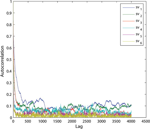
GCGC autocorrelation plot for the singular values of the cross-covariance matrix.

Figure 12.

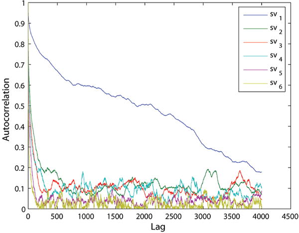
GCCG autocorrelation plot for the singular values of the cross-covariance matrix.

As can be seen in Figure 11, the autocorrelation for a GCGC sequence has singular values quickly approaching zero and remaining near zero for different values of lag. This indicates that we can assume stationarity in our molecular dynamics simulations. Similar autocorrelation plots were obtained for sequences GCAU, AUAU, and AUUA. The only exception to this is the first singular value for the GCCG helix, as shown in Figure 12. This helix cannot be assumed to have stationarity and should definitely be examined further, as the equilibrium assumption may not hold.

Normality of Molecular Dynamics Simulation

To test for normality, first a few univariate tests are performed on the six components of $g_{\mu i}=\log {(g_{\mu }^{-1}\circ g_i)}^{\vee }$. The pdf and the corresponding normal fit curves for two of the components of g_μi are plotted in Figures 13 and 14 for the GCGC helix. Similar normal probability plots are seen for the remaining four components of the GCGC helix as well as the other sequences. As in the time series calculations, g_μi represents the relative transformation from base-pair 3 to 12. The first and last two base-pairs were again excluded.

Figure 13.

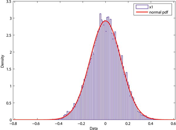
Probability density function with fit for the GCGC sequence for x₁.

Figure 14.

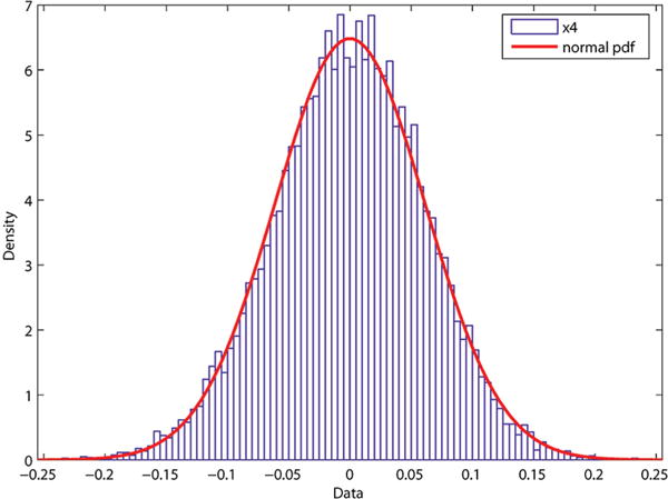
Probability density function with fit for the GCGC sequence for x₄.

To further test for normality, we use the multivariate normality test using the chi-squared plot shown in Figure 15 for the six rigid-body parameters of g_μi. The straight dashed line indicates a multivariate normal fit, and our data closely resembles this fit. Furthermore, the p-value obtained for the Chi-squared test agrees with a hypothesis of multivariate normality. Comparable results for both the univariate and multivariate fitness tests are seen for the other helix sequences.

Figure 15.

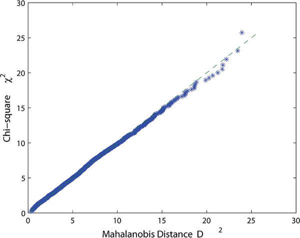
Chi-squared plot for the GCGC sequence parameters.

6. RIGID-BASE MODELS

Consider a double-helical DNA structure composed of N rigid bases, each of which can be connected to the others locally. Let the bases be numbered by the scheme shown below, where the horizontal direction indicates base pairs and vertical is the sequential direction.

$$\begin{array}{l}i+4\to i+5\\ \nwarrow \\ i+2\to i+3\\ \nwarrow \\ i\to i+1\\ \nwarrow \\ i-2\to i-1\end{array}$$

Let ${\overline{g}}_i$ denote the position and orientation of the ith such body in a static minimal energy conformation, an unperturbed state. The relative transformation between body i and body j is then ${\overline{g}}_i^{-1}\circ {\overline{g}}_j$.

Let the ith rigid body move by the small amount $\exp (X_i)\approx {\mathbb{I}}_4+X_i$, where $X_i={\sum }_{l=1}^6{x}_{i,l}{E}_l$ for $X_i^{\vee }={\mathbf{x}}_i={\left[x_{i,1},x_{i,2},\dots ,x_{i,6}\right]}^T$. Then, the relative motion between bodies i and j after the small motion is

$${[{\overline{g}}_i({\mathbb{I}}_4+X_i)]}^{-1}[{\overline{g}}_j({\mathbb{I}}_4+X_j)]=({\mathbb{I}}_4-X_i)({\overline{g}}_i^{-1}{\overline{g}}_j)({\mathbb{I}}_4+X_j)$$

Retaining terms to first order, the result can be written as

$$({\overline{g}}_i^{-1}{\overline{g}}_j)[{\mathbb{I}}_4+X_j-({\overline{g}}_i^{-1}{\overline{g}}_j^{-1})X_i({\overline{g}}_i^{-1}{\overline{g}}_j)]$$

and the change in relative pose between body i and j is

$$\mathrm{\Delta }{g}_{ij}={\mathbb{I}}_4+X_j-{({\overline{g}}_i^{-1}{\overline{g}}_j)}^{-1}{X}_i({\overline{g}}_i^{-1}{\overline{g}}_j)$$

The corresponding 6D vector of small motions is ${\mathbf{x}}_{ij}={(\mathrm{\Delta }{g}_{ij}-{\mathbb{I}}_4)}^{\vee }$ which can be written as

$${\mathbf{x}}_{ij}={\mathbf{x}}_j-\text{Ad}({\overline{g}}_j^{-1}{\overline{g}}_j){\mathbf{x}}_i$$

Given a 6 × 6 stiffness K_ij connecting these two bodies, the corresponding potential energy is

$$\begin{array}{l}{\mathcal{V}}_{ij}=\frac{1}{2}{\mathbf{x}}_{ij}^T{K}_{ij}{\mathbf{x}}_{ij}\\ =\frac{1}{2}[{\mathbf{x}}_i^T,{\mathbf{x}}_j^T]\left(\begin{array}{ll}\text{Ad}{({\overline{g}}_j^{-1}{\overline{g}}_i)}^T{K}_{ij}\text{Ad}({\overline{g}}_j^{-1}{\overline{g}}_i)\hfill & -\text{Ad}{({\overline{g}}_j^{-1}{\overline{g}}_i)}^T{K}_{ij}\hfill \\ -K_{ij}\text{Ad}({\overline{g}}_j^{-1}{\overline{g}}_i)\hfill & K_{ij}\hfill \end{array}\right)\left[\begin{array}{l}{\mathbf{x}}_i\hfill \\ {\mathbf{x}}_j\hfill \end{array}\right]\end{array}$$ (53)

and the total potential energy will be

$$\mathcal{V}={\displaystyle \sum _{i=0}^{N-2}{\displaystyle \sum _{j=i+1}^{N-1}{\mathcal{V}}_{ij}}}=\frac{1}{2}{\mathbf{x}}^T\stackrel{\sim }{K}\mathbf{x}$$ (54)

where x ∈ ℝ^6N−6 is a composite vector of all small rigid-body motions of the structure (relative to the base 0) and $\stackrel{\sim }{K}$ is a composite (6N − 6) × (6N − 6) stiffness matrix.

Equation 54 shows that the potential energy of the system run at equilibrium is in quadratic form which leads to the probability density function that will be used, the Boltzmann distribution. This corresponding conformational Boltzmann distribution is

$$f(\mathbf{x})=\frac{1}{\alpha (2k_{B}T{\stackrel{\sim }{K}}^{-1})}\exp \left(-\frac{1}{2(2k_{B}T)}{\mathbf{x}}^T\stackrel{\sim }{K}\mathbf{x}\right)$$ (55)

Here $\alpha (2k_{B}T{\stackrel{\sim }{K}}^{-1})$ is the conformational partition function that normalizes f(x) as a probability density. This is a Gaussian distribution, the covariances of which can be related to the stiffness matrix as

$$\sum ={\displaystyle {\int }_{\mathbf{x}\in {ℝ}^{6N-6}}\mathbf{x}{\mathbf{x}}^{T}f(\mathbf{x})}\mathrm{d}x=2k_{\mathrm{B}}T{\stackrel{\sim }{K}}^{-1}$$

This model can be viewed as a discrete version of the bi-rod. If Δs is the step-length between stacked bases in the continuum model and W_l, W_r, and W in sectoin 4 are viewed as being functions of the curve parameter, s, then

$$\begin{array}{l}{W}_l(p\mathrm{\Delta }s)=K_{2p,2p+2},W_r(p\mathrm{\Delta }s)=K_{2p+1,2p+3},\text{and}\\ W(p\mathrm{\Delta }s)=K_{2p,2p+1}\end{array}$$ (56)

for p ∈ {0, 1, 2, …}.

The reference frame in the middle of g₀ and g₁ defines the proximal end of the chain, and the frame in the middle of g_N−2 and g_N−1 is the distal end. Let g_d represent the frame at the “midpoint” of the distal end of the chain. The reconciliation between this model and other models results from marginalizing over all degrees of freedom except those that are present in

$$g_d={(g_0^{-1}\circ g_1)}^{-1/2}\circ g_0^{-1}\circ g_{N-2}\circ {(g_{N-2}^{-1}\circ g_{N-1})}^{1/2}$$ (57)

If we let $g_d={\overline{g}}_d(\mathbb{I}+X_d)$, then we can look at the covariance matrix Σ_d associated with x_d by determining the relationship between x_d and x₁, x_N−2, and x_N−1. We can start by letting $g_0\circ {(g_0^{-1}\circ g_1)}^{1/2}=e$ and use the referential configuration given by eqs 32 and 33. As shown in the Supporting Information, section S2, this leads to

$$\begin{array}{l}{g}_d={\overline{g}}_{N-2}[{\mathbb{I}}_4+X_{N-2}+\frac{1}{2}\log (\mathrm{trans}(w{\mathbf{e}}_1))\\ -\frac{1}{2}{X}_{N-2}\text{trans}(w{\mathbf{e}}_1)+\frac{1}{2}{X}_{N-1}\\ +\frac{5}{8}{X}_{N-2}\log (\mathrm{trans}(w{\mathbf{e}}_1))-\frac{1}{8}{X}_{N-1}\log (\mathrm{trans}(w{\mathbf{e}}_1))]\end{array}$$ (58)

and

$$\begin{array}{l}{\mathbf{x}}_d=\frac{1}{8}[3{\mathbb{I}}_4+\mathrm{Ad}(\mathrm{trans}(-w{\mathbf{e}}_1))]{\mathbf{x}}_{N-2}\\ +\frac{1}{8}[5{\mathbb{I}}_4-\mathrm{Ad}(\mathrm{trans}(-w{\mathbf{e}}_1))]{\mathbf{x}}_{N-1}\end{array}$$ (59)

Using the definition of the covariance, ${\sum }_d=\int {\mathbf{x}}_d{\mathbf{x}}_d^{T}f({\mathbf{x}}_d)d{\mathbf{x}}_d$, allows us to compute Σ_d using blocks of $(2k_{\mathrm{B}}T){\stackrel{\sim }{K}}^{-1}$. Let

$$(2k_{\mathrm{B}}T){\stackrel{\sim }{K}}^{-1}=\left(\begin{array}{lll}{\sum }_{11}\hfill & {\sum }_{12}\hfill & \dots \hfill \\ {\sum }_{12}^T\hfill & \ddots \hfill & \hfill \\ ⋮\hfill & \hfill & {\sum }_{(N-2)(N-2)}{\sum }_{(N-2)(N-1)}\hfill \\ \hfill & \hfill & {\sum }_{(N-2)(N-2)}^T{\sum }_{(N-1)(N-1)}\hfill \end{array}\right)$$

then

$$\begin{array}{l}{\sum }_d=\frac{1}{64}(A_1{\sum }_{(N-2)(N-2)}{A}_1^T+A_1{\sum }_{(N-2)(N-1)}{A}_2^T)\\ +A_2{\sum }_{(N-2)(N-1)}^T{A}_1^T+A_2{\sum }_{(N-1)(N-1)}{A}_2^T)\end{array}$$ (60)

for $A_1=3{\mathbb{I}}_4+\text{Ad}(\mathrm{trans}(-w{\mathbf{e}}_1))$ and $A_2=5{\mathbb{I}}_4-\text{Ad}(\mathrm{trans}(-w{\mathbf{e}}_1))$. This can then be used to compare the rigid-base model to other models.

One way this can be used is to compare the rigid-base model to the rigid-base-pair model. Given stiffness values for the rigid-base model, we can determine the covariance associated with x_d. If we assume that Σ_d equals Σ_data as discussed in section 5, the inverse propagation techniques in section 5.1 can be employed to determine the equivalent covariance between two adjacent base pairs for the rigid-base-pair model. This allows us to determine the stiffness between rigid-base pairs that would lead to equivalent end-to-end distributions for the rigid-base-pair model and rigid-base model.

For example, consider a rigid-base model where the “left” and “right” chain have the same stiffness such that

$$\frac{1}{2k_{\mathrm{B}}T}{K}_{2p,2p+2}=\frac{1}{2k_{B}T}{K}_{2p+1,2p+3}=\left(\begin{array}{ll}{c}_1{\mathbb{I}}_3\hfill & O\hfill \\ O\hfill & c_2{\mathbb{I}}_3\hfill \end{array}\right)$$

and the stiffness between chains is of the form

$$\frac{1}{2k_{\mathrm{B}}T}{K}_{2p,2p+1}=\left(\begin{array}{ll}{c}_3{\mathbb{I}}_3\hfill & O\hfill \\ O\hfill & c_4{\mathbb{I}}_3\hfill \end{array}\right)$$

Then, for 10 bases of B-form DNA with a width w of 2 nm, a pitch L/n of 3.4 nm, and steps δs of 0.34 nm, we obtain

$${\sum }_d={10}^{-2}\left(\begin{array}{llllll}8.4641\hfill & -0.4457\hfill & -0.0072\hfill & -0.0366\hfill & -3.9053\hfill & 0.1719\hfill \\ -0.4457\hfill & 9.1275\hfill & 0.0376\hfill & 4.9258\hfill & 0.2085\hfill & -0.0283\hfill \\ -0.0072\hfill & 0.0376\hfill & 7.5779\hfill & -0.3084\hfill & 0.0456\hfill & -0.3202\hfill \\ -0.0366\hfill & 4.9258\hfill & -0.3084\hfill & 25.0342\hfill & -0.5587\hfill & -0.0680\hfill \\ -3.9053\hfill & 0.2085\hfill & 0.0456\hfill & -0.5587\hfill & 24.4314\hfill & -0.2027\hfill \\ 0.1719\hfill & -0.0283\hfill & -0.3202\hfill & -0.0680\hfill & -0.2027\hfill & 22.6683\hfill \end{array}\right)$$

for c₁ = 20, c₂ = 10, c₃ = 5, and c₄ = 5. Using the inverse propagation technique in section 5.1 for a chain of five rigid base pairs, we calculate the covariance between base pairs to be

$${\sum }_k={10}^{-2}\left(\begin{array}{llllll}2.7254\hfill & -0.1777\hfill & -0.0113\hfill & 0.2806\hfill & -0.1961\hfill & 0.0403\hfill \\ -0.1777\hfill & 0.6725\hfill & 0.0053\hfill & -0.2313\hfill & -0.2376\hfill & 0.0398\hfill \\ -0.0113\hfill & 0.0053\hfill & 1.8945\hfill & -0.0770\hfill & -0.0765\hfill & -0.0801\hfill \\ 0.2806\hfill & -0.2313\hfill & -0.0770\hfill & 6.4387\hfill & -0.4306\hfill & 0.0322\hfill \\ -0.1961\hfill & -0.2376\hfill & -0.0765\hfill & -0.4306\hfill & 4.1842\hfill & -0.0240\hfill \\ 0.0403\hfill & 0.0398\hfill & -0.0801\hfill & 0.0322\hfill & -0.0240\hfill & 5.6671\hfill \end{array}\right)$$

This leads to an equivalent stiffness for the rigid-base-pair model of

$$\frac{1}{2k_{\mathrm{B}}T}{K}_{\text{eqiv}}={\displaystyle {\sum }_k^{-1}=\left(\begin{array}{llllll}37.2319\hfill & 4.0365\hfill & 0.2177\hfill & -1.3506\hfill & 1.8375\hfill & -0.2744\hfill \\ 4.0365\hfill & 61.0976\hfill & 0.0841\hfill & 2.2820\hfill & 3.8923\hfill & -0.4528\hfill \\ 0.2177\hfill & 0.0841\hfill & 52.8888\hfill & 0.6930\hfill & 1.0576\hfill & 0.7456\hfill \\ -1.3506\hfill & 2.2820\hfill & 0.6930\hfill & 15.7946\hfill & 1.7038\hfill & -0.0791\hfill \\ 1.8375\hfill & 3.8923\hfill & 1.0576\hfill & 1.7038\hfill & 24.4016\hfill & 0.0684\hfill \\ -0.2744\hfill & -\mathrm{0.\; 4528}\hfill & 0.7456\hfill & -0.0791\hfill & 0.0684\hfill & 17.6622\hfill \end{array}\right)}$$

Here we have illustrated a method for reconciling the rigid-base and rigid-base-pair models through the use of a frame located between the two distal bases in the rigid-base model. By comparing the statistics of this new frame with the frame attached to the distal end of a rigid-base-pair model of equal length, we can relate the stiffnesses between neighboring rigid bases to an equivalent 6D stiffness between rigid-base pairs. In this example, the equivalent stiffness was assumed to be homogeneous along the length of the equivalent rigid-base-pair model.

7. CONCLUSIONS

We have presented models of DNA and RNA at a number of scales. These models, both continuous and discrete, range from anisotropic elastic filaments (the coarsest) to rigid-base models (the finest). This spectrum of models has been unified through the use of standardized Lie group notation. Moreover, new analytical verification has been presented to reconcile and compare the different models. For example, we showed that, as expected, the bi-rod model does indeed converge to the single filament model as the filament length increases.

Additionally, molecular dynamics simulations and AFM measurements have been introduced to validate the use of some of these models. The molecular dynamics simulations and time series analysis were performed to validate the use of Gaussian models over exponential coordinates. The AFM measurements of naked and cisplatinated DNA have been shown to correspond well with the single elastic filament model in the plane. This example, which involved determining the bend angle, also highlights how these models can be used to determine physical characteristics of DNA or RNA.

Future investigations can be performed to further determine the lengths and stiffnesses for which each of these models is best suited. This may include determining how to appropriately transition from one model to another.

References

- 1.Leontis NB, Westhof E. RNA. 2001;7:499–512. doi: 10.1017/s1355838201002515. [DOI] [PMC free article] [PubMed] [Google Scholar]
- 2.Vologodskii A. Topology and Physics of Circular DNA. CRC Press; Boca Raton, FL: 1992. [Google Scholar]
- 3.Bustamante C, Marko JF, Siggia ED, Smith S. Science. 1994;265:1599–1600. doi: 10.1126/science.8079175. [DOI] [PubMed] [Google Scholar]
- 4.Bustamante C, Smith SB, Liphardt J, Smith D. Curr Opin Struct Biol. 2000;10:279–285. doi: 10.1016/s0959-440x(00)00085-3. [DOI] [PubMed] [Google Scholar]
- 5.Nelson P. Biological Physics: Energy, Information, Life. W. H. Freeman; New York: 2004. [Google Scholar]
- 6.Widom J. Q Rev Biophys. 2001;34:269–324. doi: 10.1017/s0033583501003699. [DOI] [PubMed] [Google Scholar]
- 7.Rippe K, von Hippel PH, Langowski J. Trends Biochem Sci. 1995;20:500–506. doi: 10.1016/s0968-0004(00)89117-3. [DOI] [PubMed] [Google Scholar]
- 8.Shore D, Langowski J, Baldwin RL. Proc Natl Acad Sci USA. 1981;78:4833–4837. doi: 10.1073/pnas.78.8.4833. [DOI] [PMC free article] [PubMed] [Google Scholar]
- 9.Wiggins PA, van der Heijden T, Moreno-Herrero F, Spakowitz A, Phillips R, Widom J, Dekker C, Nelson PC. Nat Nanotechnol. 2006;1:137–141. doi: 10.1038/nnano.2006.63. [DOI] [PubMed] [Google Scholar]
- 10.Cloutier TE, Widom J. Mol Cell. 2004;14:355–362. doi: 10.1016/s1097-2765(04)00210-2. [DOI] [PubMed] [Google Scholar]
- 11.Lankas F, Sponer J, Langowski J, Cheatham TE. Biophys J. 2003;85:2872–2883. doi: 10.1016/S0006-3495(03)74710-9. [DOI] [PMC free article] [PubMed] [Google Scholar]
- 12.Mazur AK. Biophys J. 2006;91:4507–4518. doi: 10.1529/biophysj.106.091280. [DOI] [PMC free article] [PubMed] [Google Scholar]
- 13.Hagerman PJ. Annu Rev Biochem. 1990;29:755–781. doi: 10.1146/annurev.bi.59.070190.003543. [DOI] [PubMed] [Google Scholar]
- 14.Okonogi TM, Alley SC, Reese AW, Hopkins PB, Robinson BH. Biophys J. 2000;78:2560–2571. doi: 10.1016/S0006-3495(00)76800-7. [DOI] [PMC free article] [PubMed] [Google Scholar]
- 15.Afonin KA, Bindewald E, Yaghoubian AJ, Voss N, Jacovetty E, Shapiro BA, Jaeger L. Nat Nanotechnol. 2010;5:676–682. doi: 10.1038/nnano.2010.160. [DOI] [PMC free article] [PubMed] [Google Scholar]
- 16.Chirikjian GS. Stochastic Models, Information Theory, and Lie Groups: Analytic Methods and Modern Applications. Vol. 2 Birkhauser; Boston, MA: 2011. [Google Scholar]
- 17.Chirikjian GS, Wang Y. Phys Rev E. 2000;62:880–892. doi: 10.1103/physreve.62.880. [DOI] [PubMed] [Google Scholar]
- 18.Chirikjian GS. J Phys: Condens Matter. 2010;22 doi: 10.1088/0953-8984/22/32/323103. [DOI] [PMC free article] [PubMed] [Google Scholar]
- 19.Coleman BD, Olson WK, Swigon D. J Chem Phys. 2003;118:7127–7140. [Google Scholar]
- 20.Mehraeen S, Sudhanshu B, Koslover EF, Spakowitz AJ. Phys Rev E. 2008;77 doi: 10.1103/PhysRevE.77.061803. [DOI] [PubMed] [Google Scholar]
- 21.Chirikjian GS, Kyatkin AB. Engineering applications of noncommutative harmonic analysis: with emphasis on rotation and motion groups. CRC Press; Boca Raton, FL: 2001. [Google Scholar]
- 22.Kleinert H. Path integrals in quantum mechanics, statistics, and polymer physics. 2nd. World Scientific; River Edge, NJ: 1995. [Google Scholar]
- 23.Odijk T. Macromolecules. 1995;28:7016–7018. [Google Scholar]
- 24.Yamakawa H. Helical wormlike chains in polymer solutions. Springer; Berlin, Germany: 1997. [Google Scholar]
- 25.Nyquist H. Phys Rev. 1928;32:110–113. [Google Scholar]
- 26.Callen HB, Welton TA. Phys Rev. 1951;83:34–40. [Google Scholar]
- 27.Chirikjian GS, Kyatkin AB. J Fourier Anal Appl. 2000;6:583–606. [Google Scholar]
- 28.Carmona M, Magasanik B. J Mol Biol. 1996;261:348–356. doi: 10.1006/jmbi.1996.0468. [DOI] [PubMed] [Google Scholar]
- 29.Crothers DM, Gartenberg MR, Shrader TE. Methods Enzymol. 1991;208:118–146. doi: 10.1016/0076-6879(91)08011-6. [DOI] [PubMed] [Google Scholar]
- 30.Erie DA, Yang G, Schultz HC, Bustamante C. Science. 1994;266:1562–1566. doi: 10.1126/science.7985026. [DOI] [PubMed] [Google Scholar]
- 31.Griffith JD, Makhov A, Zawel L, Reinberg D. J Mol Biol. 1995;246:576–584. doi: 10.1016/s0022-2836(05)80107-x. [DOI] [PubMed] [Google Scholar]
- 32.Perez-Martin J, Espinosa M. Science. 1993;260:805–807. doi: 10.1126/science.8387228. [DOI] [PubMed] [Google Scholar]
- 33.Rees WA, Keller RW, Vesenka JP, Yang G, Bustamante C. Science. 1993;260:1646–1649. doi: 10.1126/science.8503010. [DOI] [PubMed] [Google Scholar]
- 34.van der Vliet PC, Verrijzer CP. Bioessays. 1993;15:25–32. doi: 10.1002/bies.950150105. [DOI] [PubMed] [Google Scholar]
- 35.Allen DJ, Makhov A, Grilley M, Taylor J, Thresher R, Modrich P, Griffith JD. EMBO J. 1997;16:4467–4476. doi: 10.1093/emboj/16.14.4467. [DOI] [PMC free article] [PubMed] [Google Scholar]
- 36.Lobell RB, Schleif RF. Science. 1990;250:528–533. doi: 10.1126/science.2237403. [DOI] [PubMed] [Google Scholar]
- 37.Rippe K, Guthold M, von Hippel PH, Bustamante C. J Mol Biol. 1997;270:125–138. doi: 10.1006/jmbi.1997.1079. [DOI] [PubMed] [Google Scholar]
- 38.Su W, Porter S, Kustu S, Echols H. Proc Natl Acad Sci USA. 1990;87:5504–5508. doi: 10.1073/pnas.87.14.5504. [DOI] [PMC free article] [PubMed] [Google Scholar]
- 39.Wong OK, Guthold M, Erie DA, Gelles J. PLoS Biol. 2008;6:2028–2042. doi: 10.1371/journal.pbio.0060232. [DOI] [PMC free article] [PubMed] [Google Scholar]
- 40.Wyman C, Grotkopp E, Bustamante C, Nelson HC. EMBO J. 1995;14:117–123. doi: 10.1002/j.1460-2075.1995.tb06981.x. [DOI] [PMC free article] [PubMed] [Google Scholar]
- 41.Rivetti C, Guthold M. In: RNA polymerases and associated factors. Adhya SL, Garges S, editors. Vol. 370. Elsevier Academic Press; San Diego, CA: 2003. pp. 34–50. [Google Scholar]
- 42.Rivetti C, Guthold M, Bustamante C. EMBO J. 1999;18:4464–4475. doi: 10.1093/emboj/18.16.4464. [DOI] [PMC free article] [PubMed] [Google Scholar]
- 43.Guthold M, Zhu X, Rivetti C, Yang G, Thomson NH, Kasas S, Hansma HG, Smith B, Hansma PK, Bustamante C. Biophys J. 1999;77:2284–2294. doi: 10.1016/S0006-3495(99)77067-0. [DOI] [PMC free article] [PubMed] [Google Scholar]
- 44.Bustamante C, Guthold M, Zhu X, Yang G. J Biol Chem. 1999;274:16665–16668. doi: 10.1074/jbc.274.24.16665. [DOI] [PubMed] [Google Scholar]
- 45.Mirny L, Slutsky M, Wunderlich Z, Tafvizi A, Leith J, Kosmrlj A. J Phys A: Math Theor. 2009;42 [Google Scholar]
- 46.von Hippel PH, Berg OG. J Biol Chem. 1989;264:675–678. [PubMed] [Google Scholar]
- 47.Tafvizi A, Mirny LA, van Oijen AM. ChemPhysChem. 2011;12:1481–1489. doi: 10.1002/cphc.201100112. [DOI] [PMC free article] [PubMed] [Google Scholar]
- 48.Berman HM, Westbrook J, Feng Z, Gilliland G, Bhat TN, Weissig H, Shindyalov IN, Bourne PE. Nucleic Acids Res. 2000;28:235–242. doi: 10.1093/nar/28.1.235. [DOI] [PMC free article] [PubMed] [Google Scholar]
- 49.Jmol: an open-source Java viewer for chemical structures in 3D. version 12.0.41; http://www.jmol.org.
- 50.Rice PA, Yang S, Mizuuchi K, Nash HA. Cell. 1996;87:1295–1306. doi: 10.1016/s0092-8674(00)81824-3. [DOI] [PubMed] [Google Scholar]
- 51.Mouw KW, Rice PA. Mol Microbiol. 2007;63:1319–1330. doi: 10.1111/j.1365-2958.2007.05586.x. [DOI] [PubMed] [Google Scholar]
- 52.Schultz SC, Shields GC, Steitz TA. Science. 1991;253:1001–1007. doi: 10.1126/science.1653449. [DOI] [PubMed] [Google Scholar]
- 53.Abrescia NGA, Malinina L, Subirana JA. J Mol Biol. 1999;294:657–666. doi: 10.1006/jmbi.1999.3280. [DOI] [PubMed] [Google Scholar]
- 54.Todd RC, Lippard SJ. J Inorg Biochem. 2010;104:902–908. doi: 10.1016/j.jinorgbio.2010.04.005. [DOI] [PMC free article] [PubMed] [Google Scholar]
- 55.Zamble DB, Mikata Y, Eng CH, Sandman KE, Lippard S. J Inorg Biochem. 2002;91:451–462. doi: 10.1016/s0162-0134(02)00472-5. [DOI] [PubMed] [Google Scholar]
- 56.He Q, Liang CH, Lippard SJ. Proc Natl Acad Sci USA. 2000;97:5768–5772. doi: 10.1073/pnas.100108697. [DOI] [PMC free article] [PubMed] [Google Scholar]
- 57.Hambley TW. J Chem Soc, Dalton Trans. 2001:2711–2718. [Google Scholar]
- 58.Chaney SG, Campbell SL, Bassett E, Wu Y. Crit Rev Oncol Hemat. 2005;53:3–11. doi: 10.1016/j.critrevonc.2004.08.008. [DOI] [PubMed] [Google Scholar]
- 59.Lin X, Ramamurthi K, Mishima M, Kondo A, Christen RD, Howell SB. Cancer Res. 2001;61:1508–1516. [PubMed] [Google Scholar]
- 60.Raymond E, Faivre S, Chaney S, Woynarowski J, Cvitkovic E. Mol Cancer Ther. 2002;1:227–235. [PubMed] [Google Scholar]
- 61.Vaisman A, Varchenko M, Umar A, Kunkel TA, Risinger JI, Barrett JC, Hamilton TC, Chaney SG. Cancer Res. 1998;58:3579–3585. [PubMed] [Google Scholar]
- 62.Bellon SF, Coleman JH, Lippard SJ. Biochemistry. 1991;30:8026–8035. doi: 10.1021/bi00246a021. [DOI] [PubMed] [Google Scholar]
- 63.Jamieson ER, Lippard SJ. Chem Rev. 1999;99:2467–2498. doi: 10.1021/cr980421n. [DOI] [PubMed] [Google Scholar]
- 64.Pascoe JM, Roberts JJ. Biochem Pharmacol. 1974;23:1345–1357. doi: 10.1016/0006-2952(74)90354-2. [DOI] [PubMed] [Google Scholar]
- 65.Bernal-Méndez E, Boudvillain M, González-Vlchez F, Leng M. Biochemistry. 1997;36:7281–7287. doi: 10.1021/bi9703148. [DOI] [PubMed] [Google Scholar]
- 66.Kelland L. Nat Rev Cancer. 2007;7:573–584. doi: 10.1038/nrc2167. [DOI] [PubMed] [Google Scholar]
- 67.Wang D, Lippard SJ. Nat Rev Drug Discovery. 2005;4:307–320. doi: 10.1038/nrd1691. [DOI] [PubMed] [Google Scholar]
- 68.Wang H, Yang Y, Schofield MJ, Du C, Fridman Y, Lee SD, Larson ED, Drummond JT, Alani E, Hsieh P, Erie DA. Proc Natl Acad Sci USA. 2003;100:14822–14827. doi: 10.1073/pnas.2433654100. [DOI] [PMC free article] [PubMed] [Google Scholar]
- 69.Bellon SF, Lippard SJ. Biophys Chem. 1990;35:179–188. doi: 10.1016/0301-4622(90)80007-t. [DOI] [PubMed] [Google Scholar]
- 70.Gelasco A, Lippard S. J Biochemistry. 1998;37:9230–9239. doi: 10.1021/bi973176v. [DOI] [PubMed] [Google Scholar]
- 71.Stehlikova K, Kostrhunova H, Brabec V. Nucleic Acids Res. 2002;30:2894–2898. doi: 10.1093/nar/gkf405. [DOI] [PMC free article] [PubMed] [Google Scholar]
- 72.Takahara PM, Frederick CA, Lippard SJ. J Am Chem Soc. 1996;118:12309–12321. [Google Scholar]
- 73.Chirikjian GS, Wang YF. Phys Rev E. 2000;62:880–892. doi: 10.1103/physreve.62.880. [DOI] [PubMed] [Google Scholar]
- 74.Chirikjian GS, Kyatkin AB. J Fourier Anal Appl. 2000;6:583–606. [Google Scholar]
- 75.Zhou Y, Chirikjian GS. J Chem Phys. 2003;119:4962–4970. [Google Scholar]
- 76.Davies MS, Berners-Price SJ, Hambley TW. J Am Chem Soc. 1998;120:11380–11390. [Google Scholar]
- 77.Rivetti C, Guthold M, Bustamante C. J Mol Biol. 1996;264:919–932. doi: 10.1006/jmbi.1996.0687. [DOI] [PubMed] [Google Scholar]
- 78.Ansari AR, Bradley RA. Ann Math Stat. 1960;31:1174–1189. [Google Scholar]
- 79.Dutta S. Ph.D. Thesis. Wake Forest University; Winston-Salem, NC: 2011. Studying the interaction of cancer and thrombosis therapeutics with protein and DNA. [Google Scholar]
- 80.Dutta S, Rivetti C, Gassman NR, Young CG, Jones BT, Scarpinato KM. G. Analysis of single cisplatin-induced DNA bends by atomic force microscopy and simulations. Microsc Microanal. 2012 doi: 10.1002/jmr.2731. to be submitted for publication. [DOI] [PMC free article] [PubMed] [Google Scholar]
- 81.Takahara PM, Rosenzweig AC, Frederick CA, Lippard SJ. Nature. 1995;377:649–652. doi: 10.1038/377649a0. [DOI] [PubMed] [Google Scholar]
- 82.Dunham SU, Turner CJ, Lippard SJ. J Am Chem Soc. 1998;120:5395–5406. [Google Scholar]
- 83.Moakher M, Maddocks JH. Arch Ration Mech Anal. 2005;177:53–91. [Google Scholar]
- 84.Lu XJ, Babcock MS, Olson WK. J Biomol Struct Dyn. 1999;16:833–843. doi: 10.1080/07391102.1999.10508296. [DOI] [PubMed] [Google Scholar]
- 85.Wang Y, Chirikjian GS. In: Advances in Robotic Kinematics. Lenarcic J, Roth B, editors. Springer; Dordrecht, The Netherlands: 2006. pp. 95–102. [Google Scholar]
- 86.Wang Y, Chirikjian GS. IEEE Trans Robotics. 2006;22:591–602. [Google Scholar]
- 87.Wang Y, Chirikjian GS. Proceedings of the IEEE International Conference on Robotics and Automation. Orlando, FL: May 15–19, 2006. pp. 1848–1853. [Google Scholar]
- 88.Wang Y, Chirikjian GS. Int J Robotics Res. 2008;27:1258–1273. doi: 10.1177/0278364908097583. [DOI] [PMC free article] [PubMed] [Google Scholar]
- 89.Becker NB, Everaers R. Phys Rev E. 2007;76 doi: 10.1103/PhysRevE.76.021923. [DOI] [PubMed] [Google Scholar]
- 90.Becker NB, Everaers R. J Chem Phys. 2009;130 doi: 10.1063/1.3082157. [DOI] [PubMed] [Google Scholar]
- 91.Park W, Reed KB, Okamura AM, Chirikjian GS. Proceedings of the IEEE International Conference on Robotics and Automation. Anchorage, AK: May 3–7, 2010. pp. 3703–3708. [DOI] [PMC free article] [PubMed] [Google Scholar]
- 92.Lavery R, Zakrzewska K, Beveridge D, Bishop TC, Case DA, Cheatham T, III, Dixit S, Jayaram B, Lankas F, Laughton C, et al. Nucleic Acids Res. 2010;38:299–313. doi: 10.1093/nar/gkp834. [DOI] [PMC free article] [PubMed] [Google Scholar]
- 93.Lankas F, Gonzalez O, Heffler LM, Stoll G, Moakher M, Maddocks JH. Phys Chem Chem Phys. 2009;11:10565–10588. doi: 10.1039/b919565n. [DOI] [PubMed] [Google Scholar]
- 94.Case DA, Darden TA, Cheatham TE, III, Simmerling CL, Wang J, Duke RE, Luo R, Merz KM, Wang B, Pearlman DA, et al. Amber 8. University of California; San Francisco, CA: 2004. [Google Scholar]
- 95.Wang JM, Cieplak P, Kollman PA. J Comput Chem. 2000;21 [Google Scholar]
Associated Data
This section collects any data citations, data availability statements, or supplementary materials included in this article.