ChIP-BIT: Bayesian inference of target genes using a novel joint probabilistic model of ChIP-seq profiles

Abstract

Chromatin immunoprecipitation with massively parallel DNA sequencing (ChIP-seq) has greatly improved the reliability with which transcription factor binding sites (TFBSs) can be identified from genome-wide profiling studies. Many computational tools are developed to detect binding events or peaks, however the robust detection of weak binding events remains a challenge for current peak calling tools. We have developed a novel Bayesian approach (ChIP-BIT) to reliably detect TFBSs and their target genes by jointly modeling binding signal intensities and binding locations of TFBSs. Specifically, a Gaussian mixture model is used to capture both binding and background signals in sample data. As a unique feature of ChIP-BIT, background signals are modeled by a local Gaussian distribution that is accurately estimated from the input data. Extensive simulation studies showed a significantly improved performance of ChIP-BIT in target gene prediction, particularly for detecting weak binding signals at gene promoter regions. We applied ChIP-BIT to find target genes from NOTCH3 and PBX1 ChIP-seq data acquired from MCF-7 breast cancer cells. TF knockdown experiments have initially validated about 30% of co-regulated target genes identified by ChIP-BIT as being differentially expressed in MCF-7 cells. Functional analysis on these genes further revealed the existence of crosstalk between Notch and Wnt signaling pathways.

INTRODUCTION

The advent of chromatin immunoprecipitation with massively parallel DNA sequencing (ChIP-seq) has dramatically accelerated the field of genomic research in gaining an in-depth understanding of complex functions of regulatory elements in the finest scale (1). Recently, ChIP-seq profiling of eukaryote cells has been used successfully to identify histone modifications (2), distal-acting enhancers (3) and proximal transcription factor binding sites (TFBSs) at promoter regions (4). With the TFBSs identified from ChIP-seq data, it is now possible to reliably define target genes for specific transcription factors (TFs) (5). If multiple ChIP-seq data sets are available, researchers can investigate the extent of co-association among multiple TFs based on TF-gene binding patterns (6). Hence, it is important to develop accurate computational approaches for identifying binding sites and target genes from ChIP-seq data (7).

Traditionally, target genes are predicted by using peak calling methods and gene annotation tools. ChIP-seq peaks can be detected or called using MACS (8), PeakSeq (9) or other peak calling methods; peak-to-gene assignment tools such as GREAT (10) can then be used to construct a binary binding relationship with a predefined promoter region related to transcription starting site (TSS). Several computational tools have been proposed and developed to identify target genes directly from ChIP-seq data. Ouyang et al. proposed to use a weighted sum of ChIP-seq binding signals at each gene's promoter region for target gene identification (11). In their method, the regulatory effect on gene transcription (with respect to the relative location of TFBS to TSS) was modeled by an exponential distribution function. Cheng et al. proposed a probabilistic method (called TIP) to address the same problem by constructing a joint distribution of ChIP-seq binding signals and their relative locations to TSS (5). Chen et al. further improved the TIP method for target gene prediction by incorporating the significance information of peaks (12). To investigate potential association of multiple TFs, Giannopoulou et al. scored each called peak based on its location at the promoter region of a target gene and further clustered DNA-binding proteins using a non-negative matrix factorization method (6). Guo et al. proposed a generative probabilistic model to discover TF-gene binding events by integrating ChIP-seq data and DNA motif information (13). Wong et al. proposed a hierarchical model (in their SignalSpider tool) to learn TF clusters at enhancer or gene promoter regions by using multiple normalized ChIP-seq signal profiles (14).

Despite the initial success of these methods, most are developed based on available peaks by selecting highly significant signals of sample ChIP-seq data when compared with those of input data. Only TIP and SignalSpider consider the contribution of weak signals in sample ChIP-seq data. However, reliable identification of weak binding signals from background signals (i.e. non-specific binding signals) is a challenging task itself, since it requires a high sequencing depth of both sample and input ChIP-seq data sets (15). If the sequencing depth is not sufficient, existing peak detection methods return a high rate of false positives in the so-called weak binding signals. The high false positive rate makes the use of weak binding signals unreliable and impractical in such tools as TIP and SignalSpider. To reduce the false positive rate, we have proposed a novel probabilistic approach for TFBS and target gene identification where: (i) sample and input ChIP-seq data are jointly analyzed to reliably identify weak binding signals; (ii) the effect of TFBS on downstream gene transcription is also incorporated. Our proposed approach takes into account three major factors that determine the possibility of a proximal region containing a TF binding event: sample read intensity, input read intensity and relative distance of the TFBS to its TSS (16). We jointly model these three factors within a Bayesian framework, ChIP-BIT (Bayesian Inference of Target genes using ChIP-seq profiles).

The basic idea of the ChIP-BIT approach can be briefly described to highlight its novelty and uniqueness. ChIP-BIT uses a Gaussian mixture model (consisting of global and local Gaussian components) to capture both binding and background signals in the sample data. A unique feature is that the Gaussian component modeling background signals is specially designed as a local Gaussian distribution that can be estimated accurately from the input data. An exponential distribution is used to model the relative distance of TFBS to TSS, which is further incorporated into the Bayesian approach of ChIP-BIT for target gene inference. Estimated by an expectation-maximization (EM) algorithm, a posterior probability is assigned to each TFBS under consideration, indicating the likelihood of a TF-gene binding event. While genes co-regulated by a pair of TFs can be predicted using the methods introduced in (6,14), the negative impact of false positive peaks in weak binding signals cannot be ignored. For a pair of associated TFs, ChIP-BIT estimates a co-regulation probability for each common target gene based on the probabilities of individual binding events and their relative distance at promoter region.

To demonstrate the capability of ChIP-BIT on TFBS detection and target gene identification, we have applied it to several simulated or real ChIP-seq data sets with known or validated binding peaks at promoter regions, and compared its performance with several existing peak detection and gene prediction methods. For TF co-regulation identification, we have further tested ChIP-BIT on a large-scale data set consisting of over 100 ChIP-seq profiles of leukemia K562 cell line obtained from the ENCODE project (17). Finally, we have applied ChIP-BIT to an in-house ChIP-seq profiling study focused on NOTCH3 and PBX1 to help understand their functional roles in breast cancer cells. The effect of NOTCH3 and PBX1 co-regulation on target genes was investigated in conjunction with TF knockdown gene expression data. Our analysis of ChIP-seq data showed that NOTCH3 and PBX1 are also involved in the regulation of Wnt signaling pathway, indicating that crosstalk may exist between the Notch and Wnt signaling pathways.

MATERIALS AND METHODS

Workflow of the proposed approach

The workflow of the proposal approach is illustrated in Figure 1. Sample ChIP-seq data and its matched input are jointly analyzed in this framework such that a majority of mappability and GC content biases could be resolved. We first search for genomic regions with read coverage in a TF-DNA binding profile (sample ChIP-seq data) by using uniquely aligned ChIP-seq reads. After accommodating genome mappability variation, filtering out regions containing low read coverage and normalizing the control binding profile (input ChIP-seq data) against the sample data, we identify an initial set of candidate genomic regions. We then perform promoter region partition based on the UCSC hg19 RefSeq file, map candidate regions to small windows each with a size of 200 base pairs (bps), and calculate read intensities of sample and input data, respectively, in each window. Major steps of ChIP-seq data preprocessing are described in Supplementary Material S1, as shown in Supplementary Figures S1 and S2.

Figure 1.

Flowchart of the proposed ChIP-BIT approach. ChIP-BIT features (i) a joint analysis of sample and input ChIP-seq data with a unique Gaussian mixture model for transcription factor binding site (TFBS) identification, and (ii) a Bayesian framework to incorporate the location information of TFBS for target gene identification.

The proposed ChIP-BIT method is then used to compute a posterior probability for each window in order to call whether or not a window contains TFBS. Specifically, ChIP-BIT jointly analyzes sample read intensity and input read intensity using a Bayesian framework. Under the Bayesian framework, ChIP-BIT models the sample read intensity with a Gaussian mixture model, consisting of a global Gaussian component for binding signals and a local Gaussian component for background signals. Importantly, the local Gaussian component can be accurately estimated from the input read intensity, making it possible to detect weak binding signals reliably because of the lower false positive rate. The relative distance of TFBS to TSS is modeled by an exponential distribution function and incorporated into the Bayesian approach of ChIP-BIT for target gene inference. An EM algorithm estimates a posterior probability that each window contains a true TFBS for target gene regulation. Windows with posterior probabilities over a predefined probability threshold are merged together if they are continuous. The merged windows are finally reported as TFBSs for potential binding events to occur, and their associated target genes are also reported accordingly. In Supplementary Material S2, an overall workflow of the ChIP-BIT implementation is shown in Supplementary Figure S3; the formats of its input and output files are summarized in Supplementary Table S1. Additionally for core functions of ChIP-BIT, an example including input and output signals is shown in Supplementary Figure S4.

Model description of ChIP-BIT

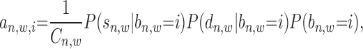
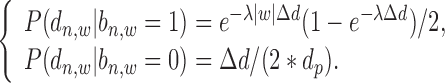
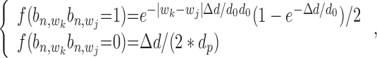
We define the scale of promoter region as ±10k bps from the TSS (5) and divide each promoter region into small non-overlapping windows. For ChIP-seq data analysis, the window-based approach has been used in several peak detection methods including SICER (18), BCP (19) and HOMER (20). To use a standard way to incorporate the information of relative distance to the TSS, we choose a window size of 200 bps to define a basic window unit, whose midpoint to TSS is defined as the relative distance for all binding signals falling in this window. We map candidate enriched regions to windows and use read intensity , the natural log of the read coverage, to represent the read enrichment status in each window, as shown in Figure 2.

Figure 2.

Model description of ChIP-BIT on TFBS detection and target gene identification. A ‘red’ bar represents the read intensity of a TFBS and a ‘blue’ bar represents the read intensity of a background region. Those ‘gray’ bars represent input signals at the same locations of any ‘red’ or ‘blue’ bars. For each window, read intensities from sample and input data are jointly analyzed for reliable TFBS identification; relative distance to (transcription starting site) TSS is also considered in a Bayesian framework for target gene prediction.

ChIP-seq data can be treated as a mixture of TFBSs and background signals. Background signals are fully represented in the input data, but TFBSs need to be distinguished from background signals in the sample data. Hence, each enriched region has two hidden states: binding occurrence and non-occurrence , with probabilities and , respectively. The sum of these two probabilities equals to 1. If , this region is more likely to contain a TFBS, shown as a ‘red’ bar in Figure 2; otherwise, it is a background region, shown as a ‘blue’ bar in Figure 2. Read intensity is a major signature to help identify TFBS. The value of read intensity in the sample data (‘red’ or ‘blue’ bars) and its differentiation against from the input data (‘gray’ bars) altogether determine whether or not this binding event truly occurs. The regulatory effect of peaks on target gene transcription also must be considered for TFBS prediction. This effect is mainly reflected by the relative distance of to its nearest TSS. The shorter is, the more possible is sampled from an effective TFBS, shown as the ‘red’ curve in Figure 2. However, if comes from a background region, no matter where it is located, its contribution to gene regulation is non-informative (the ‘blue’ curve in Figure 2). We have developed a probabilistic approach using a Bayesian framework to achieve TFBS detection and target gene identification simultaneously.

Bayesian framework for TFBS and target gene prediction

We use to index target genes and to index windows at the -th gene promoter region. The binding variable has two hidden states as binding occurrence () and non-binding occurrence (). Each binding variable () has three observations as read intensity in the sample data, read intensity in the input data, and binding location information (referring to as the relative distance to TSS). For each = 1 or 0, we define a posterior probability as:

(1)

Given an enriched window, the relationship between its binding signal intensity and relative distance to TSS is assumed to be conditionally independent. Then, Equation (1) can be extended as:

(2)

where 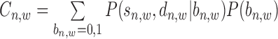is a normalization factor.

Based on the available literature and real data examinations, read intensity follows a mixture Gaussian distribution (14), as and in Figure 2. More details about how to calculate read intensity can be found in Supplementary Material S3 (see Supplementary Figure S5 for an illustration and Supplementary Figure S6 for an example). The conditional probability in Equation (2) can be calculated as:

(3)

where for , is sequenced from a TFBS so it follows a global Gaussian distribution with mean and variance ; while for , is sequenced from background region so it follows a local Gaussian distribution with mean (its input signal) and variance . is the variance of background signals, which can be directly calculated from the input data. The values of and are both unknown and need to be estimated from all with state .

The second conditional probability in (2), , is determined by the relative distance to TSS as well as the binding state . is defined as the distance between middle point of the -th window to TSS of -th gene.

(4)

where denotes window size, and = . The total number of windows at one side of promoter, , is defined by . represents the length of half promoter region (positive side or negative side to TSS). We set = 200 bps and = 10k bps for all the experiments conducted in this paper.

The regulatory effect of a TFBS on its target gene decays exponentially when increases (6,7,11,21,22). This decaying effect is TF specific (11) and the parameter of its exponential distribution needs to be properly optimized so as to provide the most reliable gene prediction performance (6) (which has been demonstrated to be better than binary peak-gene assignment (7)). We have examined this feature in real ChIP-seq data of TFs under different conditions using similar ways as in (21,22) (Supplementary Material S3). From Supplementary Figures S7 and S8, it can be clearly seen that the average read enrichment in sample ChIP-seq data follows an exponential distribution along gene promoter region while this distribution in input ChIP-seq data is relatively uniform. When is very large, the read enrichment of ChIP-seq binding is much lower than that at proximal regions. Since different TFs may have different features on their binding signal location distributions at promoter region, a parameter is introduced as shown in Equation (5):

(5)

Parameter needs to be estimated from all with . Detailed derivation of Equation (5) can be found in Supplementary Material S4 and Supplementary Figure S9. For , is treated as background signal so that is assumed to follow a uniform distribution with a discrete probability density function .

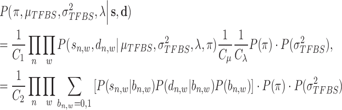
For the prior probability in Equation (2), since there is no prior knowledge about the proportion of regions that containing TFBSs, we define the prior probability as

(6)

From the above discussion, we have formulated the TFBS detection problem as a parameter estimation problem: how to estimate parameters , , and hence to calculate the posterior probability . We assume uniform prior on , uniform prior on , inverse Gamma prior on (conjugate prior of Gaussian distribution) and Beta prior on  (conjugate prior of Binomial distribution) as follows (23):

(7)

(8)

(9)

(10)

where and are hyper-parameters for inverse Gamma distribution and and are hyper-parameters for Beta distribution.

We assume inverse Gamma distribution on variance because we want to limit most binding signals around . This is consistent with the ChIP-seq data generation process, since most segments selected (‘picked up’) by the antibody are sequenced to a similar depth. Some background regions are also sequenced by the machine but, due to the lack of antibody selection, their sequence depth is lower than binding regions. In addition, after read tag assembly, there are usually some segments showing extremely high coverage. As demonstrated in (24), these regions are mainly caused by segment duplication (high copy number), not TF-specific binding locations. Therefore, we assume an inverse Gamma distribution on to lower the impact of noise on TFBS binding signal distribution estimation.

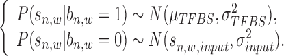
To estimate the parameters described above, we define a second posterior probability as

(11)

where and are constant values.

Within this Bayesian framework, we can estimate all parameters (, , and ) and the posterior probability () using an EM approach. We set the initial values of all to 0.5, beta distribution parameters and to 5.0, and inverse gamma distribution parameters and to 1.0. Then, we carry out the E-step and the M-step iteratively to estimate all parameters until the improvement of the posterior probability defined in Equation (11) is less than 1.0e-6. The E-step and M-step are mathematically detailed as follows:

E-step:

(12)

M-step:

(13)

(14)

(15)

(16)

Based on our experiments on several ChIP-seq data sets, iteration of the E-step and the M-step usually converges within 50 rounds. More detailed deviation about the estimation of each parameter in Equations (12–16) can be found in Supplementary Material S5. For ChIP-seq data analysis, we select as high confident binding events those windows whose probabilities are over 0.9. Since each binding event has been associated with a target gene, we obtain a target gene list as identified for a particular TF under investigation.

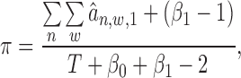
Co-regulated target gene prediction

For a pair of TFs of interest, based on the results of ChIP-BIT, we can also calculate the probability for each common target gene to reveal the two TFs’ co-regulatory effect on gene transcription. After processing the ChIP-seq data for each TF using ChIP-BIT, we extract all enriched windows whose probabilities are larger than a threshold of 0.5. For each gene, if multiple windows are enriched at it promoter region, we select the window with the highest probability to denote both binding location and binding confidence. We define a variable with two states as co-regulation occurrence ( = 1) and non-occurrence ( = 0) for -th TF and -th TF at the promoter region of -th target gene. Then, the posterior probability for is defined by

(17)

where and denote window indices of -th TF and -th TF, respectively. Candidate states for , , are (1,1,1), (0,1,0), (0,0,1) and (0,0,0). Alternatively, these are two states: = 1 and = 0.

The conditional probability with state (1,1,1) depends on the relative distance of two binding sites in the same gene's promoter region. If these binding sites are proximal, e.g. within 1k bps, the likelihood for co-regulation occurrence will be high. If these sites are located distantly, their co-regulation likelihood will be low. For all other states with = 0, no co-regulation event occurs; hence, this likelihood function is not dependent on any distance information. We assume an exponential distribution for the likelihood with state = 1, and an uniform distribution for the likelihood with state = 0 as in the following equation:

(18)

where is an effective region parameter that is set to 1k bps.

Probability (or 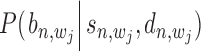) represents the posterior probability for each binding event of -th TF (or -th TF), which can be estimated as (or ) using Equation (12). With these two probabilities and with incorporated into Equation (17), the co-regulation probability with state (1,1,1) can be calculated as follows:

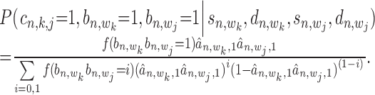(19)

Consequently, common target genes co-regulated by both TFs can be ranked according to the posterior probability calculated in Equation (19).

RESULTS

To demonstrate the effectiveness of ChIP-BIT on TFBS (or peak) and target gene prediction, we tested ChIP-BIT on simulated and experimental ChIP-Seq data sets and compared the results with several available peak-calling methods including MACS, PeakSeq, BCP, Dfilter and MOSAiCS. MACS (8) and PeakSeq (9) are the two most widely used peak calling methods; these tools use local Poisson or Binomial statistics to identify enriched peaks. BCP (19) uses a Bayesian change point approach to model read coverage change along the genome and identifies peak boundaries. Dfilter (25) calculates the form of an optimal detection filter with reads from input data and then applies this filter to reads from sample data for peak prediction. MOSAiCS (26) uses a negative binomial mixture model to identify enriched windows based on read counts from sample and input data. The detailed parameters used to run each tool can be found in Supplementary Material S6.

Performance evaluation by realistic simulation studies

We generated a list of realistic genomic regions by applying PeakSeq (9) to MYC ChIP-seq data acquired from a leukemia study of cell line K562 in the ENCODE project (http://genome.ucsc.edu/ENCODE/). We selected those peaks falling on chromosome 1 and mapped them to the UCSC hg19 RefSeq file. Consistent with our model design, we set the promoter region as ±10k bps around TSS for this simulation study. We observed an exponential-like distribution of the relative distances of these peaks to the TSS. Then, about 6000 proximal peaks in promoter regions were extracted for simulation data generation. We randomly selected half of the peaks as ‘true’ peaks and treated the remaining regions as ‘background’. Using a simulation tool developed in (27), we simulated sample data and input data with the same total number of reads (denoted as Case 1). Read intensities of peaks or background regions and their relative distance TSS can be found in Supplementary Material S7, Supplementary Figure S10A and C. We called peaks by using ChIP-BIT and other comparable peak calling tools; a successful call is counted if a detected peak overlaps with any ‘true’ peak in the promoter region. The precision/recall performances of ChIP-BIT and other competing methods on peak detection are shown in Figure 3. Note that the denominator used in the precision calculation is the number of peaks within the promoter regions. From Figure 3A, we can see that the precision/recall performance of ChIP-BIT is the best in Case 1, where the joint model of sample and input data and informative distance distribution significantly promote the precision of ChIP-BIT. As shown in Figure 3B, ChIP-BIT has a strong detection capability on weak binding signals (whose read intensity are lower than the mean value of read intensities in sample data), which promotes the overall performance of ChIP-BIT. Read intensities and relative distances to TSS of peaks detected by ChIP-BIT can be found in Supplementary Material S7, Supplementary Figure S10B and D.

Figure 3.

Precision and recall performance of ChIP-BIT and existing peak calling methods on simulated ChIP-seq data. (A) Detection performance on all peaks in simulation Case 1; (B) detection performance on weak binding signals in simulation Case 1; (C) detection performance on all peaks in simulation Case 2; (D) detection performance on weak binding signals in simulation Case 2; (E) false positive rate of the detected weak binding signals in simulation Case 1; (F) false positive rate of the detected weak binding signals in simulation Case 2.

To show that ChIP-BIT still works well when the relative distance distribution is more uniform (rather than exponential) along the promoter region, we simulated another pair of data sets (denoted as Case 2) based on genomic regions enriched in our in-house NOTCH3 ChIP-seq data acquired from MCF-7 breast cancer cells. In Case 2, when the distribution of peaks along the promoter region is more uniform and the read intensity difference between TFBSs and background regions is smaller (Supplementary Material S7, Supplementary Figure S11), the overall detection performance of ChIP-BIT on simulated peaks in promoter regions is still better than competing methods, as shown in Figure 3C. The performance improvement in Case 2 mainly reflects joint modeling of read intensities from the sample and input data. The Gaussian mixture model has enabled ChIP-BIT to detect more weak binding signals at promoter regions than any other existing method, as clearly shown in Figure 3D.

F-measure was calculated as 2*precision*recall/(precision+recall) to assess the overall performance of each method, as summarized in Table 1 for all the methods in comparison. From Figure 3A–D and Table 1, it can be seen that the detection performance of ChIP-BIT on simulated peaks in the gene promoter region is better than existing peak callers, especially in terms of its detection performance on weak binding signals. In Figure 3E and F, we further present the false positive rate of weak binding signals as detected by each method, when the overall precision (precision on all peaks) is fixed at the same level (in a range of 0.70–0.95) for all the methods in comparison. From the figures, we can clearly see that ChIP-BIT has the lowest false positive rate on the detected weak binding signals, a major benefit of ChIP-BIT's joint modeling of the sample and input data. We also calculated the F-measure of each peak caller under default or recommended settings for TF peak detection, as shown in Supplementary Material S7, Supplementary Tables S2 and S3. It can be found that ChIP-BIT achieves the highest performance in both cases. Consequently, in this stimulation study, the ability of ChIP-BIT in differing binding sites from background regions at gene promoter region is better than other competing methods, resulting in an improved performance of ChIP-BIT.

Table 1. Overall precision-recall performance, F-measure, on peak detection.

Method	ChIP-BIT	MOSAiCS	PeakSeq	MACS	BCP	Dfilter
Case 1 (all peaks)	0.9045	0.8477	0.8289	0.8100	0.8076	0.7932
Case 1 (weak binding signals)	0.8318	0.7989	0.7352	0.7700	0.7493	0.7452
Case 2 (all peaks)	0.9078	0.8179	0.8398	0.8123	0.8037	0.7664
Case 2 (weak binding signals)	0.8328	0.7775	0.7084	0.7692	0.7253	0.7233

Accuracy of the peak boundary detection for those correctly called peaks (denoted by the overlap proportion between detected peaks and ground truth) also must be evaluated. ChIP-BIT does not emphasize boundary detection, due to its use of a window based genome partition, but how much it covers background regions (precision) or cuts off binding effective regions (recall) needs to be quantitatively evaluated. We summarized the performance of peak boundary detection for different methods in Supplementary Material S7, Supplementary Tables S4 and S5. The highest precision value of ChIP-BIT demonstrated its capability to identify sharp peaks. The recall performance of ChIP-BIT was mainly caused by the low read intensity at peak boundaries. The other methods, except for PeakSeq, reported a high recall value but a much lower precision, indicating that they captured some background regions close to the binding site. The overall peak length distributions of ‘true’ peaks and peaks called by each method are shown in Supplementary Material S7, Supplementary Figures S12 and S13. It can be found that most of the true peaks are quite sharp with length smaller than 500 bps. ChIP-BIT and PeakSeq provided similar peak length distributions to that of the true peaks, while peak length distributions of the other methods had an overall shift to the ‘wide’ region.

Finally, we compared the performance of ChIP-BIT for target gene prediction with that of method as proposed by Ouyang et al. (11), TIP as proposed in (5) and its improved version as proposed in (12). In the previous simulation study of ChIP-BIT, we set the candidate promoter region as ±10k bps from TSS. However, the true promoter region might be closer to TSS, e.g. ±5k bps, ±2k bps or even less. In real data analysis, it has been noted that different promoter regions may provide different results for target gene prediction (5,10). To evaluate the performance for different promoter regions, we therefore generated another two simulation cases for either Case 1 or 2 with ‘true’ peaks within ±5k bps or ±2k bps promoter from the TSS, respectively (in addition to the simulation data of ±10k bps promoter region). We applied ChIP-BIT, method proposed by Ouyang et al., TIP and improved TIP to each data set for target gene prediction. The area under the ROC curve (AUC) values are summarized in Table 2. As shown in Supplementary Material S7, Supplementary Figure S14, the performance of method proposed by Ouyang et al. is sensitive to the speed of its exponential decaying weight function. Thus, we tested multiple values of exponential decaying speed and presented the best performance in Table 2. ChIP-BIT outperformed the three peer methods. Interestingly, in Case 1 the performance of TIP or its improved version increases when the region of true binding signals gets closer to the TSS, but their performance degrades in Case 2. After detailed examination, we found that in Case 1 the location-specific weight distribution learned by TIP has a sharp peak around TSS, as shown in Supplementary Material S7, Supplementary Figure S15A and B. Therefore, if ‘true’ TFBSs are located close to the TSS, TIP can predict target gene more accurately. However, in Case 2 binding signals are spread across all promoter regions more evenly. In this case, the location-specific weight learned by TIP is more uniformly distributed along the promoter region, as shown in Supplementary Material S7, Supplementary Figure S15C and D. If ‘true’ binding sites are located very close to the TSS, such as within ±2k bps, and TIP is used to predict target genes, the contamination of background signals distant to TSS will be significant because the sum of weight within ±2k bps is not significantly higher than that from ±2k bps to ±10k bps. In real genomic studies, there is often no prior knowledge of the binding signal distribution around TSS, and knowledge of the length of promoter regions is also limited. Under such practical conditions, ChIP-BIT would have a more robust performance for target gene identification than the other existing methods.

Table 2. AUC performance on target gene prediction.

Method	Case 1			Case 2
	Promoter region			Promoter region
	±10k bps	±5k bps	±2k bps	±10k bps	±5k bps	±2k bps
ChIP-BIT	0.923	0.948	0.972	0.943	0.972	0.982
Ouyang	0.730	0.801	0.846	0.819	0.836	0.892
Improved TIP	0.786	0.839	0.875	0.896	0.855	0.810
TIP	0.698	0.753	0.812	0.819	0.822	0.797

Performance comparison using real ChIP-seq data

It is a challenging task to validate a large number of TFBSs identified from ChIP-seq data. Several metrics have been used in ChIP-seq studies to tackle this challenge, including motif enrichment, ChIP-qPCR, benchmark of peaks, TF knockdown with small interfering RNA (siRNA) or short hairpin RNA (shRNA) followed by RNA-seq profiling, enrichment of histone modification or methylation signals and functional enrichment of target genes. In this study, we compared the results of different peak calling methods on validated benchmark of peaks, target genes identified through TF knockdown with shRNA followed by RNA-seq profiling and enrichment of histone modification for active promoters.

Benchmarks of three TFs, MAX, NRSF and SRF, have been manually curated by Rye et al. (28) using their ChIP-seq data. We downloaded the ChIP-seq data and the benchmarks of MAX, NRSF and SRF (28). All peak calling methods were run with default or recommended settings for TFBS identification. For each TF, using results of PeakSeq we calculated the proportion of peaks within gene promoter regions among peaks detected from the whole genome, as shown in Supplementary Material S8, Supplementary Figure S16. For these three TFs, on average ∼50% of peaks are located at gene promoter regions. Then, we performed a filtering step on both benchmarks and identified peaks of each method using gene promoter regions for a fair comparison between ChIP-BIT and competing methods. Numbers of filtered benchmark regions and peaks are summarized in Supplementary Material S8, Supplementary Tables S6 and S7. For each TF, read intensities of peaks identified by ChIP-BIT in sample or input data are shown in Supplementary Material S8, Figures S17–S19. Furthermore, the rates of false positives (peaks overlapping with ‘negative’ regions), calculated according to the definition in (28) each time a new true positive (peak overlapping with a ‘positive’ region) is encountered, are shown in Figure 4A–C, for MAX, NRSF and SRF, respectively. As we can see from Figure 4A, all the methods worked well with a very similar performance in detecting peaks of MAX in promoter regions. As shown in Figure 4B, ChIP-BIT had a significantly lower false positive rate than others on detecting proximal peaks of NRSF. ChIP-BIT also exhibited a better performance than most of the competing methods for proximal peak detection of SRF (see Figure 4C).

Figure 4.

Performance comparison using real ChIP-seq data. (A) False positive rate of K562 MAX peaks; (B) False positive rate of K562 NRSF peaks; (C) False positive rate of Gm12878 SRF peaks; (D) Average overlap of RNA-seq validated target genes of each method; (E) Overlap rate of promoter bound peaks with H3K4me3 enriched active promoters; (F) Overlap rate of promoter bound peaks of PcG proteins with bivalent promoters enriched by both H3K4me3 and H3K27me3.

To compare the prediction performance of different methods in identifying target genes, we downloaded K562 cell line ATF3, EGR1 and SRF ChIP-seq data from the ENCODE project and the matched RNA-seq data before or after specific short hairpin RNA (shRNA) treatment for each TF (GEO access number GSE33816). For these specific TFs, on average ∼55% of peaks are identified from gene promoter regions, as shown in Supplementary Material S8, Supplementary Figure S20. TF-specific shRNA shall efficiently lower (with at least a 70% reduction) the expression of the protein of interest. We compared the prediction performance of different methods in terms of differentially expressed downstream target genes when a specific upstream regulator was knocked down. Detailed procedures to identify differentially expressed genes using RNA-seq data can be found in Supplementary Material S8.2 and the heatmap of the identified target genes can be found in Supplementary Figure S21. Specifically, we selected two peak callers, PeakSeq and MACS, for TFBS prediction using ChIP-seq data as they have been widely used in the ENCODE project. The identified peaks were annotated using GREAT (10) for target gene prediction. TIP was also applied to each ChIP-seq sample data to predict target genes directly. Numbers of ChIP-seq target genes and those differentially expressed ones are summarized in Supplementary Material S8, Supplementary Tables S8–S10. It can be found that the rate of differentially expressed genes among all ChIP-seq targets is ∼10–15%, regardless of the varying number of target genes predicted by individual method. This is consistent to previous observations that about 14.7% of target genes were differentially expressed following the knockdown of a specific TF (29). However, TIP had a relatively lower rate, indicating a higher false positive rate due to that no ChIP-seq input data were used. Since there was no ground truth of target genes, we compared the ‘average overlap with other methods’ (i.e. proportion of target genes overlapped with other methods) on those differentially expressed target genes identified by each method, as shown in Figure 4D. We assumed that ‘true’ target genes should be differentially expressed when its regulator was knocked down and be detected more consistently using different methods. Note that the measure of ‘average overlap with other methods’ has been used for peak comparison among different peak calling approaches when ground truth evidence is not available (30). As shown in Figure 4D, ChIP-BIT exhibited the highest average overlap while TIP, using sample ChIP-seq data only, had the lowest average overlap for all three TFs.

Finally, we investigated the enrichment of ‘active’ marker H3K4me3 at promoter bound peaks identified by each peak calling method. It has been demonstrated that about 91% of all the Pol II islands are correlated with H3K4me3 islands, and H3K4me3 enrichment correlates with gene expression positively (31). Therefore, H3K4me3 enrichment can be used as a positive indicator to locate active bindings at target gene promoters. We downloaded H3K4me3 enriched regions of the same cell line, K562, from the ENCODE project and calculated the average overlap rate (defined by the number of promoter bound peaks overlapped with H3K4me3 enrichment divided by the number of all promoter bound peaks) of the five TFs (ATF3, EGR1, MAX, NRSF and SRF) for each peak calling method. It can be seen from Figure 4E that peaks identified by ChIP-BIT had a significantly higher overlap rate with H3K4me3 enriched regions than the other methods. Hence, ChIP-BIT, by incorporating distance-based regulatory effect on target genes, shows its effectiveness in locating active bindings of TFs as indicted by the H3K4me3 enrichment.

TF co-association clusters in Leukemia K562 cell line

We applied ChIP-BIT to a large-scale ChIP-seq data set (with 117 ChIP-seq profiles of leukemia K562 cell line 17) to demonstrate its usefulness for binding site identification. With the binding sites identified by ChIP-BIT, we then studied the co-association relationship among the 117 TFs profiled. TF co-association on leukemia cell line K562 has been investigated by the ENCODE group (17), where MACS and PeakSeq were used as the major peak calling tools. It is reported that over 40% of the reported peaks are within ±2.5k bps of TSS. In this paper, for those representative TFs, 50–60% of peaks are identified in gene promoter regions when a larger promoter region (±10k bps from TSS) is investigated (resulting in an increase of (at least) 10% peaks identified). We applied ChIP-BIT to an updated data collection including 117 ChIP-seq data sets and selected peaks with a probability ≥0.9 to generate a TF co-association map by following the same strategy (17). Several clustering approaches including hierarchical clustering (32), affinity propagation clustering (33) and k-means (34) were carried out in our study to identify those robust TF clusters. A TF co-association map can be found in Supplementary Material S8.3, Supplementary Figure S22.

We compared our clustering results with the original clusters (17). Six of the clusters, C1–C6, show a very high similarity with the original clusters. Cluster C7 is a unique one and includes SUZ12, EZH2, RNF2, CBX2 and CBX8. These TFs are mainly members of Polycomb-group (PcG) complex and their ChIP-seq profiles were lately added to the ENCODE ChIP-seq data set (they were not included in the original work). From our clustering analysis of the binding sites, this PcG complex shows a robust and unique pattern as its binding event occurs in leukemia cells. Therefore, all clusters identified here are either consistent with the original clusters reported (Cluster C1–C6) or well supported by available biological knowledge on members of the PcG (Cluster C7). In summary, ChIP-BIT not only can identify TF binding sites from ChIP-seq profiles effectively, but can it also provide reliable TF co-association pattern from large-scale ChIP-seq profiling studies based the important binding information captured.

We also compared the peak detection results from different peak calling methods on the Cluster C7 consisting of PcG proteins. PcG proteins usually serve as transcriptional repressors and bind at bivalent domain to poise the transcription of regulatory genes (35). Bivalent domain is a particular chromatin signature at promoter region that harbors histone modifications of both ‘repressive’ marker H3K27me3 and ‘active’ marker H3K4me3 (36). Thus, this signature can be used to examine PcG's TFBSs in support of their transcriptional regulation. We downloaded the enriched regions of H3K27me3 and H3K4me3 of K562 cell line from the ENCODE project and mapped the identified peaks of each TF in Cluster C7 to bivalent promoters enriched by both H3K27me3 and H3K4me3. The average overlap rate (as defined by the number of promoter bound peaks overlapping with bivalent domain divided by the number of all promoter bound peaks) of each method is shown in Figure 4F. It can be seen from the figure that ChIP-BIT showed a higher overlap rate with bivalent domain than that of the other competing methods.

Association between PBX1 and NOTCH3 in breast cancer

NOTCH3-mediated signaling plays an important role in the proliferation of breast cancer cells and has emerged as a possible therapeutic target (37). In this signaling pathway, previously we reported that PBX1 is a target of NOTCH3 in ovarian cancer (38). An interaction of PBX1 and NOTCH3 in breast cancer cells is implied by the correlation of their gene expression data and the target genes identified from PBX1 ChIP-seq data (39); NOTCH3 and PBX1 control the expression of a large number of genes associated with endocrine therapy resistance in breast cancer cells. We have acquired NOTCH3 ChIP-seq data from MCF-7 breast cancer cells to further investigate the association between PBX1 and NOTCH3. The raw distributions of read intensity and relative distance to TSS for NOTCH3 or PBX1 can be found in Supplementary Material S9, Supplementary Figure S23. Most binding sites of PBX1 are located quite close to the TSS, while binding sites of NOTCH3 are distributed more evenly across the promoter region. Additionally, the read intensity distributions of the peaks detected by ChIP-BIT using different thresholds can be found in Supplementary Material S9, Supplementary Table S11.

Following the procedure shown in Figure 1, we identified 2871 target genes by applying ChIP-BIT to NOTCH3 ChIP-seq data. We also applied ChIP-BIT to a PBX1 ChIP-Seq data set acquired from MCF-7 cells (39) and identified 5280 target genes in total. For comparison, we called peaks using PeakSeq or MACS and predicted target genes using GREAT by setting promoter regions as ±10k bps to the TSS. TIP was applied to the sample ChIP-seq data only to directly predict target genes. Results of peak calling and gene identification using different methods can be found in Supplementary Material S9, Supplementary Tables S12 and S13. Since PeakSeq reports read enrichment in sample or input ChIP-seq data for each detected peak, its read intensity distributions of the detected peaks are comparatively shown with those of ChIP-BIT for NOTCH3 or PBX1 in Figure 5.

Figure 5.

Peak calling results of NOTCH3 or PBX1 by using ChIP-BIT and PeakSeq. (A) Read intensities of PeakSeq detected NOTCH3 peaks in sample data (red) and input data (gray); (B) read intensities of ChIP-BIT detected NOTCH3 peaks; (C) relative distances of ChIP-BIT detected peaks to TSS; (D), (E) and (F) represent the same set of information obtained from PBX1 ChIP-seq data analysis as that of (A), (B) and (C).

Read intensity distributions of NOTCH3 peaks reported by PeakSeq and ChIP-BIT are shown in Figure 5A and B, respectively. We can see from Figure 5B that ChIP-BIT separates binding signals from sample and input data sets quite well. Although some peaks have relative ‘weak’ enrichment in the NOTCH3 sample profile, their fold changes are large enough for peak calling. The average fold change of read enrichment between sample and input data is 6.57 for the NOTCH3 peaks identified by ChIP-BIT, which is higher than a commonly used fold change threshold of 4. Even though our exponential distribution assumption assigns higher weights to those peaks close to the TSS, as shown in Figure 5C, some relatively distant peaks can still be detected if their enrichment in the sample data is significantly higher than that in input data. For PBX1, ChIP-BIT also provides a better separation of sample and input binding signals as well, as shown in Figure 5E. The average fold change of read enrichment between sample and input data is 7.26 for the PBX1 peaks identified by ChIP-BIT, also much higher than a commonly used fold change threshold of 4. By comparing Figure 5F–C, we can see that TFBS location-wise distributions are different for different TFs.

For target gene prediction, similar to previous real data analysis on K562 cell line, we present the average gene overlap rate of a particular method to the other methods in Supplementary Material S9, Supplementary Table S13. ChIP-BIT has the highest average overlap rate among all four methods for either NOTCH3 or PBX1. Moreover, by applying functional enrichment analysis using QIAGEN's Ingenuity Pathway Analysis (http://www.ingenuity.com) and DAVID (http://david.abcc.ncifcrf.gov) on NOTCH3 target genes in the NCI/Nature interaction, QIAGEN pathway and KEGG pathway databases (links to pathway databases can be found in Supplementary Material S10), we identified 22 Notch signaling pathway genes from the NOTCH3 target gene list of ChIP-BIT (P-value: 1.5e-2). For the target genes obtained by other methods (i.e. PeakSeq, MACS and TIP), as shown in Supplementary Material S10, Supplementary Table S16, the enrichment of Notch signaling pathway is much less significant in terms of the number of genes or the statistical significance (P-value). Furthermore, to identify target genes co-regulated by NOTCH3 and PBX1, we calculated the posterior probability for each common target (Equation (19)), as shown in Supplementary Material S10, Supplementary Figure S24. By setting the threshold at 0.95, in total we identified 621 NOTCH3-PBX1 co-regulated target genes. ChIP-BIT identified target genes regulated by NOTCH3, PBX1 or both can be found in Supplementary Material, Supplementary Table S14. Note that for other methods (PeakSeq, MACS and TIP), we directly took the intersection of two gene lists identified from NOTCH3 and PBX1 ChIP-Seq data as the co-regulated target genes; the number of co-regulated target genes is shown in Supplementary Material S10, Supplementary Table S15.

It has been known that Notch and Wnt signaling pathways share some common functions (40) and cooperate in breast and ovarian cancers (41,42). Both pathways are related to cancer stem cells, which are regarded as a main source of cancer recurrence and chemo-resistance (43). Functional enrichment analysis on ChIP-BIT identified NOTCH3-PBX1 co-regulated target genes highlights enrichment of the Notch signaling pathway (P-value: 1.5e-3), including ARNT, BLOC1S1, CNTN1, DLL4, DTX4, FIGF, HES1, HEY1, NCOA1, NOTCH4 and RBPJ, and Wnt signaling pathway (P-value: 4.7e-2), including CEBPD, IL6, KLF5, PIAS1, PRICKLE1, SMAD4, SOX2, SOX9, WNT2, WNT2B and WNT4. The details of the enriched pathways can be found in Supplementary Material S10, Supplementary Figures S25 and S26. However, the enrichment of these two pathways from the target genes identified by other methods (i.e. PeakSeq, MACS and TIP) is much lower, as shown in Supplementary Material S10, Supplementary Tables S17 and S18. Binding sites of NOTCH3 and PBX1 on selected co-regulated target genes identified by ChIP-BIT are shown in Figure 6. In summary, the functional enrichment of key pathways (i.e. Notch and Wnt) from the identified targets by ChIP-BIT is more significant than that from other competing methods.

Figure 6.

Binding signals of PBX1 (blue) and NOTCH3 (red) on selected target genes. (A) HES1, (B) RBPJ and (C) HEY1 are known key genes in Notch signaling pathway; (D) WNT2B, (E) PIAS1 and (F) SOX9 are known key genes in Wnt signaling pathway.

Target gene validation using TF knockdown experiments

As an initial step to validate the ChIP-BIT identified target genes co-regulated by NOTCH3 and PBX1, we used gene expression data acquired from inhibition and knockdown experiments of NOTCH3 and PBX1. First, we inhibited Notch signaling with 1 μM GSI (γ-secretase inhibitor I, EMD Chemicals, San Diego, CA, USA), a well-known Notch signaling inhibitor (38), for 48 h; both NOTCH3 and PBX1 are inhibited by GSI. Since most ChIP-seq target genes are marginally differentially expressed (29), we set a relatively low fold change threshold, 1.3 (0.3 in its log2 format), for differential expression analysis. A total of 331 (53%) of ChIP-BIT identified NOTCH3-PBX1 co-regulated target genes are differentially expressed. More details about the differentially expressed target gene identification can be found in Supplementary Material S11.

Second, we used small interfering RNA (siRNA) to knockdown NOTCH3 and PBX1 specifically, since siRNAs are more specific inhibitors of NOTCH3 and PBX1 than the GSI. PBX1 knockdown experiment using siPBX1 was performed previously and microarray gene expression data were made available to us by the authors (39). In this study, we further knocked down NOTCH3 using siNOTCH3 and acquired gene expression data for NOTCH3-PBX1 co-regulated target gene validation. For the knockdown experiment, MCF-7 cells were transfected with NOTCH3 siRNA for 48 h followed by Western blotting to confirm the knockdown efficiency as shown in Figure 7A. NOTCH3 expression was clearly inhibited with siNOTCH3 compared with its negative control.

Figure 7.

TF knockdown experiments for target gene validation. (A) Western blot of NOTCH3 protein expression after transfecting MCF-7 breast cancer cells with siRNA of NOTCH3 and scramble (SCR) for 48 h, including full length (FL), transmembrane form (TM) and intracellular domain (ICD); (B) mRNA expression levels of PBX1 and NOTCH3 across siRNA samples; (C) mRNA expression pattern of functional PBX1-NOTCH3 co-regulated target genes, which is shown in terms of the fold change (log2) of expression level for each TF knockdown experiment.

We then performed microarray mRNA profiling by using Illumina HumanHT-12 v4 Expression BeadChip before and after siNOTCH3 is introduced to the cells. Under each condition, we generated two replicates. The normalized mRNA expression of NOTCH3 for each siRNA sample is shown in Figure 7B. NOTCH3 expression was down regulated significantly (P-value 9.7e-3) with siNOTCH3.

Among the common genes targeted by NOTCH3-PBX1, gene transcription can be regulated by PBX1, NOTCH3 or both, as illustrated in Supplementary Material S11, Supplementary Figure S27. Knockdown of either TF will provide a set of differentially expressed genes among 621 co-regulated target genes, but these two sets of genes are not necessarily the same. With a predefined fold change threshold of 1.3 (0.3 in log2 format), there are 62 genes differentially expressed in the siPBX1 sample, 81 genes differentially expressed in the siNOTCH3 sample and 50 genes differentially expressed in both siRNA samples. A total of 193 (30%) of target genes are differentially expressed. It is expected that a majority of genes identified from siRNA experiments be also differently expressed after GSI treatment because GSI will inhibit both PBX1 and NOTCH3 simultaneously (as described before). After comparing to the differentially expressed genes (331 genes) with or without GSI treatment, we found 149 genes that overlapped, as shown in Supplementary Material S11, Supplementary Figure S28. Differentially expressed gene list under each condition is summarized in Supplementary Material, Supplementary Table S19. Functional enrichment analysis was carried out on these 149 differentially expressed NOTCH3-PBX1 co-regulated target genes. Notch signaling pathway including BLOC1S1, CNTN1, HEY1, NCOA1, RBPJ and Wnt signaling pathway including CEBPD, IL6, PIAS1, PRICKLE1, SOX2, SOX9 are enriched with P-values of 6.7e-4 and 3.2e-3, respectively. Fold changes (before and after siRNA transfection) of these functional target genes’ expression are presented in Figure 7C, where other co-regulated target genes involved in these two pathways (identified from previous section) are also listed, although their gene expression changes are less significant.

In summary, with our ChIP-seq profiling study, we have shown that both Notch and Wnt signaling pathways are enriched among functional target genes co-regulated by NOTCH3 and PBX1. While further biological validation experiments are likely needed, our computational analysis supports the hypothesis that crosstalk between these two pathways may exist downstream of transcription factors PBX1 and NOTCH3. The existence of such crosstalk would require further experiments for biological validation so as to establish the association of Notch and Wnt signaling pathways with the development and progression of breast cancer.

DISCUSSION

In this paper, a Bayesian approach, ChIP-BIT, was developed and applied to identify ChIP-seq binding peaks and their target genes. While there are a few peak calling tools like PeakSeq or MACS available for ChIP-seq data analysis, by using the same peak annotation tool as GREAT it appears that the target genes they report are different. Differences in input-sample data normalization, background region filtering, wide peak partition, mathematical models and thresholds for peak selection likely explain the final differences in target gene identification. Our objective was to identify ChIP-Seq peaks and target genes simultaneously using an integrative approach rather than taking multiple independent steps.

In contrast to conventional peak detection methods, ChIP-BIT will compute a probability for each peak reported rather than a significance P-value. All peaks are modeled with a global probabilistic model so that probabilities of different peaks are directly comparable. Strong or weak binding signals are defined according to their read intensities in the sample ChIP-seq data. Weak binding regions have an overall lower read intensity in the sample ChIP-seq data but as TF specific binding sites, compared to the low local input signal, their fold changes are still significant. Such weak binding signals can be used in any post-processing step by incorporating their probabilities of binding occurrences. In addition, ChIP-BIT predicts TFBSs and target genes simultaneously, where each TFBS has been assigned to a target gene. As a straightforward extension, for a pair of TFs, their co-regulated target genes can be called based on the probabilities reported by ChIP-BIT. Rather than using peak overlap or gene overlap, we model each co-binding event using the probability for each binding and their relative distance at gene's promoter region. Finally, ChIP-BIT assigns each common target gene a probability indicating the co-regulation strength of both TFs.

The method is applied to identify peaks that lay in promoter regions around TSSs, whose results can be easily integrated with gene expression data for functional target gene identification or gene regulatory network inference. Those target genes with a high probability can be validated by using ChIP-qPCR to show the existence of specific TF binding signals at their promoter region. In addition, genes identified from cell line studies can be further investigated among tumor samples acquired from patients. However, due to the limited scale of the promoter region (±10k) and sharp peak preference, the proposed method cannot be directly applied to identify distant enhancers or broad histone modifications. As enhancers or histone modifications may be located quite distant from a gene's TSS, or cover the whole gene body, these are usually investigated without an emphasis on target gene association. To address this problem, we will modify the ChIP-BIT algorithm in the future to find an alternative solution to distance-free enriched region detection.

In summary, to identify target genes associated with TFBSs, we have developed a probabilistic method called ChIP-BIT to identify ChIP-seq enriched peaks. Each peak is annotated by a target gene and more importantly, has a probability reflecting its binding strength. ChIP-BIT is a novel Bayesian approach in that (i) a Gaussian mixture model is developed to help improve weak binding event detection; (ii) an exponential distribution is incorporated to model the effect of TFBSs on their target gene transcription. Through simulation studies, we have demonstrated that ChIP-BIT distinguishes enriched peaks especially those weak ones from background signals better than most available tools. By using ChIP-BIT to identify target genes co-regulated by both PBX1 and NOTCH3 in MCF-7 cells, we have found that there is a significant interaction between PBX1 and NOTCH3 on target gene regulation. Functional enrichment analysis in breast cancer cells supports crosstalk between the Wnt signaling and Notch signaling pathways downstream of PBX1 and NOTCH3.

AVAILABILITY

MATLAB and R scripts of ChIP-BIT are made available to the research community, which can be downloaded at http://www.cbil.ece.vt.edu/software.htm.

SUPPLEMENTARY DATA

Supplementary Data are available at NAR Online.

FUNDING

National Institutes of Health (NIH) [CA149653 and CA164384 to J.X., CA149147 and CA184902 to R.C., NS29525–18 to Y.W., CA148826 and CA187512 to T.-L.W. in part]. Funding for open access charge: National Institutes of Health (NIH) [CA149653] and Virginia Tech's Open Access Subvention Found (VT OASF).

Conflict of interest statement. None declared.

REFERENCES

- 1.Encode Project Consortium. An integrated encyclopedia of DNA elements in the human genome. Nature. 2012;489:57–74. doi: 10.1038/nature11247. [DOI] [PMC free article] [PubMed] [Google Scholar]
- 2.Wang J., Lunyak V.V., Jordan I.K. BroadPeak: a novel algorithm for identifying broad peaks in diffuse ChIP-seq datasets. Bioinformatics. 2013;29:492–493. doi: 10.1093/bioinformatics/bts722. [DOI] [PubMed] [Google Scholar]
- 3.Visel A., Rubin E.M., Pennacchio L.A. Genomic views of distant-acting enhancers. Nature. 2009;461:199–205. doi: 10.1038/nature08451. [DOI] [PMC free article] [PubMed] [Google Scholar]
- 4.Heidari N., Phanstiel D.H., He C., Grubert F., Jahanbani F., Kasowski M., Zhang M.Q., Snyder M.P. Genome-wide map of regulatory interactions in the human genome. Genome Res. 2014;24:1905–1917. doi: 10.1101/gr.176586.114. [DOI] [PMC free article] [PubMed] [Google Scholar]
- 5.Cheng C., Min R., Gerstein M. TIP: a probabilistic method for identifying transcription factor target genes from ChIP-seq binding profiles. Bioinformatics. 2011;27:3221–3227. doi: 10.1093/bioinformatics/btr552. [DOI] [PMC free article] [PubMed] [Google Scholar]
- 6.Giannopoulou E.G., Elemento O. Inferring chromatin-bound protein complexes from genome-wide binding assays. Genome Res. 2013;23:1295–1306. doi: 10.1101/gr.149419.112. [DOI] [PMC free article] [PubMed] [Google Scholar]
- 7.Sikora-Wohlfeld W., Ackermann M., Christodoulou E.G., Singaravelu K., Beyer A. Assessing computational methods for transcription factor target gene identification based on ChIP-seq data. PLoS Comput. Biol. 2013;9:e1003342. doi: 10.1371/journal.pcbi.1003342. [DOI] [PMC free article] [PubMed] [Google Scholar]
- 8.Zhang Y., Liu T., Meyer C.A., Eeckhoute J., Johnson D.S., Bernstein B.E., Nusbaum C., Myers R.M., Brown M., Li W., et al. Model-based analysis of ChIP-Seq (MACS) Genome Biol. 2008;9:R137. doi: 10.1186/gb-2008-9-9-r137. [DOI] [PMC free article] [PubMed] [Google Scholar]
- 9.Rozowsky J., Euskirchen G., Auerbach R.K., Zhang Z.D., Gibson T., Bjornson R., Carriero N., Snyder M., Gerstein M.B. PeakSeq enables systematic scoring of ChIP-seq experiments relative to controls. Nat. Biotechnol. 2009;27:66–75. doi: 10.1038/nbt.1518. [DOI] [PMC free article] [PubMed] [Google Scholar]
- 10.McLean C.Y., Bristor D., Hiller M., Clarke S.L., Schaar B.T., Lowe C.B., Wenger A.M., Bejerano G. GREAT improves functional interpretation of cis-regulatory regions. Nat. Biotechnol. 2010;28:495–501. doi: 10.1038/nbt.1630. [DOI] [PMC free article] [PubMed] [Google Scholar]
- 11.Ouyang Z., Zhou Q., Wong W.H. ChIP-Seq of transcription factors predicts absolute and differential gene expression in embryonic stem cells. Proc. Natl. Acad. Sci. U.S.A. 2009;106:21521–21526. doi: 10.1073/pnas.0904863106. [DOI] [PMC free article] [PubMed] [Google Scholar]
- 12.Chen X., Shi X., Shajahan-Haq A.N., Hilakivi-Clarke L., Clarke R., Xuan J.H. Statistical identification of co-regulatory gene modules using multiple ChIP-Seq experiments. Bioinformatics 2014: Proceedings of the International Conference on Bioinformatics Models, Methods and Algorithms. 2014:109–116. [Google Scholar]
- 13.Guo Y., Mahony S., Gifford D.K. High resolution genome wide binding event finding and motif discovery reveals transcription factor spatial binding constraints. PLoS Comput. Biol. 2012;8:e1002638. doi: 10.1371/journal.pcbi.1002638. [DOI] [PMC free article] [PubMed] [Google Scholar]
- 14.Wong K.C., Li Y., Peng C., Zhang Z. SignalSpider: probabilistic pattern discovery on multiple normalized ChIP-Seq signal profiles. Bioinformatics. 2015;31:17–24. doi: 10.1093/bioinformatics/btu604. [DOI] [PubMed] [Google Scholar]
- 15.Xu H., Handoko L., Wei X., Ye C., Sheng J., Wei C.L., Lin F., Sung W.K. A signal-noise model for significance analysis of ChIP-seq with negative control. Bioinformatics. 2010;26:1199–1204. doi: 10.1093/bioinformatics/btq128. [DOI] [PubMed] [Google Scholar]
- 16.Budden D.M., Hurley D.G., Crampin E.J. Predictive modelling of gene expression from transcriptional regulatory elements. Brief. Bioinform. 2014;16:616–628. doi: 10.1093/bib/bbu034. [DOI] [PubMed] [Google Scholar]
- 17.Gerstein M.B., Kundaje A., Hariharan M., Landt S.G., Yan K.K., Cheng C., Mu X.J., Khurana E., Rozowsky J., Alexander R., et al. Architecture of the human regulatory network derived from ENCODE data. Nature. 2012;489:91–100. doi: 10.1038/nature11245. [DOI] [PMC free article] [PubMed] [Google Scholar]
- 18.Zang C., Schones D.E., Zeng C., Cui K., Zhao K., Peng W. A clustering approach for identification of enriched domains from histone modification ChIP-Seq data. Bioinformatics. 2009;25:1952–1958. doi: 10.1093/bioinformatics/btp340. [DOI] [PMC free article] [PubMed] [Google Scholar]
- 19.Xing H., Mo Y., Liao W., Zhang M.Q. Genome-wide localization of protein-DNA binding and histone modification by a Bayesian change-point method with ChIP-seq data. PLoS Comput. Biol. 2012;8:e1002613. doi: 10.1371/journal.pcbi.1002613. [DOI] [PMC free article] [PubMed] [Google Scholar]
- 20.Heinz S., Benner C., Spann N., Bertolino E., Lin Y.C., Laslo P., Cheng J.X., Murre C., Singh H., Glass C.K. Simple combinations of lineage-determining transcription factors prime cis-regulatory elements required for macrophage and B cell identities. Mol. Cell. 2010;38:576–589. doi: 10.1016/j.molcel.2010.05.004. [DOI] [PMC free article] [PubMed] [Google Scholar]
- 21.Mokry M., Hatzis P., Schuijers J., Lansu N., Ruzius F.P., Clevers H., Cuppen E. Integrated genome-wide analysis of transcription factor occupancy, RNA polymerase II binding and steady-state RNA levels identify differentially regulated functional gene classes. Nucleic Acids Res. 2012;40:148–158. doi: 10.1093/nar/gkr720. [DOI] [PMC free article] [PubMed] [Google Scholar]
- 22.Cheng C., Gerstein M. Modeling the relative relationship of transcription factor binding and histone modifications to gene expression levels in mouse embryonic stem cells. Nucleic Acids Res. 2012;40:553–568. doi: 10.1093/nar/gkr752. [DOI] [PMC free article] [PubMed] [Google Scholar]
- 23.Sun N., Carroll R.J., Zhao H. Bayesian error analysis model for reconstructing transcriptional regulatory networks. Proc. Natl. Acad. Sci. U.S.A. 2006;103:7988–7993. doi: 10.1073/pnas.0600164103. [DOI] [PMC free article] [PubMed] [Google Scholar]
- 24.Pickrell J.K., Gaffney D.J., Gilad Y., Pritchard J.K. False positive peaks in ChIP-seq and other sequencing-based functional assays caused by unannotated high copy number regions. Bioinformatics. 2011;27:2144–2146. doi: 10.1093/bioinformatics/btr354. [DOI] [PMC free article] [PubMed] [Google Scholar]
- 25.Kumar V., Muratani M., Rayan N.A., Kraus P., Lufkin T., Ng H.H., Prabhakar S. Uniform, optimal signal processing of mapped deep-sequencing data. Nat. Biotechnol. 2013;31:615–622. doi: 10.1038/nbt.2596. [DOI] [PubMed] [Google Scholar]
- 26.Kuan P.F., Chung D.J., Pan G.J., Thomson J.A., Stewart R., Keles S. A statistical framework for the analysis of ChIP-Seq data. J. Am. Stat. Assoc. 2011;106:891–903. doi: 10.1198/jasa.2011.ap09706. [DOI] [PMC free article] [PubMed] [Google Scholar]
- 27.Zhang Z.D., Rozowsky J., Snyder M., Chang J., Gerstein M. Modeling ChIP sequencing in silico with applications. PLoS Comput. Biol. 2008;4:e1000158. doi: 10.1371/journal.pcbi.1000158. [DOI] [PMC free article] [PubMed] [Google Scholar]
- 28.Rye M.B., Saetrom P., Drablos F. A manually curated ChIP-seq benchmark demonstrates room for improvement in current peak-finder programs. Nucleic Acids Res. 2011;39:e25. doi: 10.1093/nar/gkq1187. [DOI] [PMC free article] [PubMed] [Google Scholar]
- 29.Cusanovich D.A., Pavlovic B., Pritchard J.K., Gilad Y. The functional consequences of variation in transcription factor binding. PLoS Genet. 2014;10:e1004226. doi: 10.1371/journal.pgen.1004226. [DOI] [PMC free article] [PubMed] [Google Scholar]
- 30.Laajala T.D., Raghav S., Tuomela S., Lahesmaa R., Aittokallio T., Elo L.L. A practical comparison of methods for detecting transcription factor binding sites in ChIP-seq experiments. BMC Genomics. 2009;10:618. doi: 10.1186/1471-2164-10-618. [DOI] [PMC free article] [PubMed] [Google Scholar]
- 31.Barski A., Cuddapah S., Cui K., Roh T.Y., Schones D.E., Wang Z., Wei G., Chepelev I., Zhao K. High-resolution profiling of histone methylations in the human genome. Cell. 2007;129:823–837. doi: 10.1016/j.cell.2007.05.009. [DOI] [PubMed] [Google Scholar]
- 32.Eisen M.B., Spellman P.T., Brown P.O., Botstein D. Cluster analysis and display of genome-wide expression patterns. Proc. Natl. Acad. Sci. U.S.A. 1998;95:14863–14868. doi: 10.1073/pnas.95.25.14863. [DOI] [PMC free article] [PubMed] [Google Scholar]
- 33.Frey B.J., Dueck D. Clustering by passing messages between data points. Science. 2007;315:972–976. doi: 10.1126/science.1136800. [DOI] [PubMed] [Google Scholar]
- 34.Quackenbush J. Computational analysis of microarray data. Nat. Rev. Genet. 2001;2:418–427. doi: 10.1038/35076576. [DOI] [PubMed] [Google Scholar]
- 35.Di Croce L., Helin K. Transcriptional regulation by Polycomb group proteins. Nat. Struct. Mol. Biol. 2013;20:1147–1155. doi: 10.1038/nsmb.2669. [DOI] [PubMed] [Google Scholar]
- 36.Voigt P., Tee W.W., Reinberg D. A double take on bivalent promoters. Genes Dev. 2013;27:1318–1338. doi: 10.1101/gad.219626.113. [DOI] [PMC free article] [PubMed] [Google Scholar]
- 37.Yamaguchi N., Oyama T., Ito E., Satoh H., Azuma S., Hayashi M., Shimizu K., Honma R., Yanagisawa Y., Nishikawa A., et al. NOTCH3 signaling pathway plays crucial roles in the proliferation of ErbB2-negative human breast cancer cells. Cancer Res. 2008;68:1881–1888. doi: 10.1158/0008-5472.CAN-07-1597. [DOI] [PubMed] [Google Scholar]
- 38.Park J.T., Shih Ie M., Wang T.L. Identification of Pbx1, a potential oncogene, as a Notch3 target gene in ovarian cancer. Cancer Res. 2008;68:8852–8860. doi: 10.1158/0008-5472.CAN-08-0517. [DOI] [PMC free article] [PubMed] [Google Scholar]
- 39.Magnani L., Stoeck A., Zhang X., Lanczky A., Mirabella A.C., Wang T.L., Gyorffy B., Lupien M. Genome-wide reprogramming of the chromatin landscape underlies endocrine therapy resistance in breast cancer. Proc. Natl. Acad. Sci. U.S.A. 2013;110:E1490–E1499. doi: 10.1073/pnas.1219992110. [DOI] [PMC free article] [PubMed] [Google Scholar]
- 40.Hayward P., Kalmar T., Arias A.M. Wnt/Notch signalling and information processing during development. Development. 2008;135:411–424. doi: 10.1242/dev.000505. [DOI] [PubMed] [Google Scholar]
- 41.Collu G.M., Brennan K. Cooperation between Wnt and Notch signalling in human breast cancer. Breast Cancer Res. 2007;9:105. doi: 10.1186/bcr1671. [DOI] [PMC free article] [PubMed] [Google Scholar]
- 42.Chen X., Stoeck A., Lee S.J., Shih Ie M., Wang M.M., Wang T.L. Jagged1 expression regulated by Notch3 and Wnt/beta-catenin signaling pathways in ovarian cancer. Oncotarget. 2010;1:210–218. doi: 10.18632/oncotarget.127. [DOI] [PMC free article] [PubMed] [Google Scholar]
- 43.Takebe N., Harris P.J., Warren R.Q., Ivy S.P. Targeting cancer stem cells by inhibiting Wnt, Notch, and Hedgehog pathways. Nat. Rev. Clin. Oncol. 2011;8:97–106. doi: 10.1038/nrclinonc.2010.196. [DOI] [PubMed] [Google Scholar]
Associated Data
This section collects any data citations, data availability statements, or supplementary materials included in this article.