High-Resolution ¹H-MRSI of the Brain Using SPICE: Data Acquisition and Image Reconstruction

Abstract

Purpose

To develop data acquisition and image reconstruction methods to enable high-resolution ¹H MR spectroscopic imaging (MRSI) of the brain, using the recently proposed subspace-based spectroscopic imaging framework called SPICE (SPectroscopic Imaging by exploiting spatiospectral CorrElation).

Theory and Methods

SPICE is characterized by the use of a subspace model for both data acquisition and image reconstruction. For data acquisition, we propose a novel spatiospectral encoding scheme that provides hybrid data sets for determining the subspace structure and for image reconstruction using the subspace model. More specifically, we use a hybrid chemical shift imaging (CSI)/echo-planar spectroscopic imaging (EPSI) sequence for two-dimensional (2D) MRSI and a dual-density, dual-speed EPSI sequence for three-dimensional (3D) MRSI. For image reconstruction, we propose a method that can determine the subspace structure and the high-resolution spatiospectral reconstruction from the hybrid data sets generated by the proposed sequences, incorporating field inhomogeneity correction and edge-preserving regularization.

Results

Phantom and in vivo brain experiments were performed to evaluate the performance of the proposed method. For 2D MRSI experiments, SPICE is able to produce high SNR spatiospectral distributions with an approximately 3 mm nominal in-plane resolution from a 10-min acquisition. For 3D MRSI experiments, SPICE is able to achieve an approximately 3 mm in-plane and 4 mm through-plane resolution in about 25 min.

Conclusion

Special data acquisition and reconstruction methods have been developed for high-resolution ¹H-MRSI of the brain using SPICE. Using these methods, SPICE is able to produce spatiospectral distributions of ¹H metabolites in the brain with high spatial resolution, while maintaining a good SNR. These capabilities should prove useful for practical applications of SPICE.

INTRODUCTION

Significant efforts have been made in the last several decades to achieve fast, high-resolution MR spectroscopic imaging (MRSI), through the development of fast sequences (1–10) and advanced image reconstruction methods (11–25). SPICE (SPectroscopic Imaging by exploiting spatiospectral CorrElation) is a relatively new approach that we recently proposed to achieve high-resolution MRSI with good signal-to-noise ratio (SNR) and speed (26). A key feature of SPICE is the use of a subspace model for both data acquisition and image reconstruction. Specifically, SPICE proposes a novel spatiospectral encoding strategy to generate hybrid data sets, from which the subspace structure and the spatiospectral distribution are recovered. In this work, we present pulse sequences and algorithms to implement SPICE for high-resolution¹H-MRSI of the brain.

One practical issue in SPICE data acquisition lies in balancing the resolution, speed, and SNR tradeoff when acquiring the hybrid data sets for subspace determination and for subspace-based reconstruction, respectively. To this end, we propose a hybrid chemical shift imaging (CSI)/echo-planar spectroscopic imaging (EPSI) sequence to achieve an extended (k,t)-space coverage in a short acquisition period for 2D MRSI using SPICE. The CSI component has limited k-space coverage but high SNR, and uses the entire free induction decay (FID) period for spectral encoding; it is used to acquire the data needed for accurate subspace estimation (denoted as ${\mathcal{D}}_1$). The EPSI component has high data acquisition speed and allows an extended k-space coverage within a short period; it is used to acquire the data needed for high-resolution spatiospectral reconstruction (denoted as ${\mathcal{D}}_2$). For 3D MRSI using SPICE, however, this sequence may be too slow for practical applications. To address this issue, we propose a dual-density, dual-speed sequence that performs a hybrid of slow EPSI scans (to acquire ${\mathcal{D}}_1$) and rapid EPSI-like scans (to acquire ${\mathcal{D}}_2$), which benefits from the increased sensitivity offered by 3D encoding. The proposed hybrid sampling scheme, enabled by the subspace model, effectively combines the advantages of slow scans (i.e., high SNR and full spectral encoding) and rapid scans (i.e., high resolution) for accelerated MRSI using sparse sampling.

Given the (k,t)-space data acquired using the proposed acquisition scheme, the main issues for SPICE reconstruction are estimation of the subspace structure (or the basis spanning the low- dimensional subspace) from ${\mathcal{D}}_1$ and reconstruction of the underlying spatiospectral/spatiotemporal function from ${\mathcal{D}}_2$. A key problem in subspace estimation is the removal of B₀ field inhomogeneity effects from the limited k-space data. Assuming the availability of a high-resolution field map, we utilize a regularized super-resolution reconstruction scheme to solve this problem. With the subspace determined from the field corrected data, the reconstruction problem can be translated into the estimation of a set of spatial coefficients, with a significantly reduced number of degrees-of-freedom compared to the high-dimensional spatiospectral/spatiotemporal function of interest (making possible a high SNR reconstruction from the very noisy and sparse data). This problem can then be solved using a regularized linear least-squares formulation that incorporates an explicit low-rank model as well as the capability to incorporate field inhomogeneity correction and edge-preserving regularization. The use of regularization not only serves to stabilize the coefficient estimation problem but also enables the incorporation of additional prior information for improved reconstruction.

We have obtained results from both phantom and healthy volunteers to evaluate the performance and in vivo feasibility of the proposed SPICE data acquisition and image reconstruction methods. In particular, for in vivo 2D MRSI experiments, the proposed method is able to produce¹H metabolite maps with an 80 × 80 matrix size over a 220 × 220mm² field of view (FOV) with an 8 mm slice thickness (i.e., a nominal 2.75 mm in-plane resolution) in a 10-minute acquisition with a similar SNR to an equivalent-time CSI scan. For in vivo 3D MRSI experiments, the proposed method is able to produce metabolite distributions with an 80 × 80 × 20 matrix size over a 240 × 240 × 72 mm³ FOV (i.e., a nominal 3 mm in-plane and 3.6 mm through-plane resolution) in a 25-minute acquisition. In the subsequent sections, the proposed acquisition and reconstruction methods are described in detail, and accompanied by some representative results.

THEORY

Subspace Model

SPICE exploits the spatiotemporal partial separability (PS) of high-dimensional spectroscopic signals and models the spatiotemporal function ρ (r; t) (the Fourier counterpart of the underlying spatiospectral function of interest $\stackrel{\sim }{\rho }(\mathbf{r},f))$ as (26–29)

$$\rho \left(\mathbf{r},t\right)={\displaystyle \sum _{l=1}^L{c}_l}\left(\mathbf{r}\right){\varphi }_l\left(t\right)={\displaystyle \sum _{l_1=1}^{L_1}{c}_{l_1}}\left(\mathbf{r}\right){\varphi }_{l_1}\left(t\right)+{\displaystyle \sum _{l_2=1}^{L_2}{c}_{l_2}\left(\mathbf{r}\right)}{\varphi }_{l_2}\left(t\right),$$ [1]

where ${\left\{{\varphi }_{l_1}\right(t\left)\right\}}_{l_1=1}^{L_1}$ and ${\left\{{\varphi }_{l_2}\right(t\left)\right\}}_{l_2=1}^{L_2}$ represent the sets of temporal basis functions for the metabo lite signal of interest and the “nuisance” signals (e.g., the water, lipid, and baseline signals), ${\left\{c_{l_1}\right(\mathbf{r}\left)\right\}}_{l_1=1}^{L_1}$ and ${\left\{c_{l_2}\right(\mathbf{r}\left)\right\}}_{l_2=1}^{L_2}$ the corresponding spatial coefficients, and L₁ and L₂ the model or ders (typically a small number) for each signal component. Note that the PS model in Eq. [1] implies that the following Casorati matrix formed from ρ (r; t) over any point set ${\left\{\right({\mathbf{r}}_n,t_m\left)\right\}}_{n,m=1}^{N,M}$

$$\rho =\left[\begin{array}{cccc}\rho \left({\mathbf{r}}_1,t_1\right)& \rho \left({\mathbf{r}}_1,t_2\right)& \dots & \rho \left({\mathbf{r}}_1,t_M\right)\\ \rho \left({\mathbf{r}}_2,t_1\right)& \rho \left({\mathbf{r}}_2,t_2\right)& \dots & \rho \left({\mathbf{r}}_2,t_M\right)\\ ⋮& ⋮& \ddots & ⋮\\ \rho \left({\mathbf{r}}_N,t_1\right)& \rho \left({\mathbf{r}}_N,t_2\right)& \dots & \rho \left({\mathbf{r}}_N,t_M\right)\end{array}\right]$$

is low rank (with the rank upper-bounded by the model order). This model significantly reduces the number of degrees-of-freedom in the imaging problem, providing a better tradeoff for SNR, resolution, and speed. Furthermore, it decouples the spatial and temporal variations of ρ (r, t), thus enabling special methods for both data acquisition and image reconstruction to achieve fast, high-resolution MRSI with good SNR. The proposed data acquisition and reconstruction methods are described in the subsequent sections.

Data Acquisition

The low-dimensional subspace/low-rank model described above presents new flexibilities for spatiospectral encoding, which are not available with the conventional Fourier model. One straightforward approach to using the model for accelerating data acquisition is to perform a random undersampling in the corresponding (k,t)-space of ρ (r, t) and perform low-rank matrix recovery to jointly determine ϕ_l(t) and c_l(r) from the undersampled data. Although such a joint subspace pursuit and reconstruction approach has been successfully used in various dynamic imaging applications (e.g., (30–32)), it is not effective for high-resolution in vivo MRSI due to the limited SNR. An alternative is to acquire complementary data sets that allows for determining ϕ_l(t) and c_l(r) separately. Such a scheme is desirable because if ϕ_l(t) is predetermined, a high SNR and high-resolution reconstruction can be obtained from sparse and very noisy data by estimating only c_l(r). Figure 1 compares these two scenarios in a simulation setting to demonstrate this point, using a numerical phantom with additional features to increase the spatiospectral complexity (Details on the numerical phantom can be found in (26, 28)). The gold standard (first row in Fig. 1) has a rank of 8. A noisy data set was generated by adding complex white Gaussian noise onto the noiseless spatiotemporal distribution. The results from a rank-8 truncation of the noisy data (third row in Fig. 1) represent the best one can do if jointly estimating ϕ_l(t) and c_l(r) from a single very noisy data set (in the maximum likelihood sense). By comparing them to the images in the last row obtained by projecting the noisy data onto the predetermined subspace, we can observe that the subspace model with known subspace structure clearly leads to better recovered spatiospectral features. It is worth noting that the acquisition of complementary data sets also supports joint determination of ϕ_l(t) and c_l(r).

Figure 1.

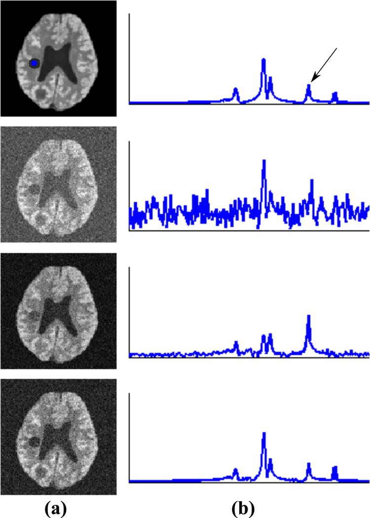
Illustration of two different scenarios for data acquisition consideration (see text) in a simulation setting: (a) the spatial maps for the spectral component identified by the arrow (in b) from the gold standard (first row), a fully sampled noisy data set (second row), a rank-8 truncation of the noisy data (third row), and the projection of the same noisy data onto the known subspace (fourth row); (b) the spectra for each case from the voxels whose locations are indicated by the blue dot. As can be seen, for the case where the spatial coefficients and subspace are jointly estimated from very noisy data (third row), strong spectral distortion is observed. This highlights the importance of an accurate predetermined subspace.

To implement the above described hybrid acquisition strategy, we propose a hybrid CSI/EPSI sequence for 2D MRSI using SPICE. The proposed sequence is shown in Fig. 2a, where the CSI component is used to obtain ${\mathcal{D}}_1$ for determining ϕ_l(t) (subspace), and the EPSI component is used to obtain ${\mathcal{D}}_2$ for determining c_l(r) (spatial coefficients). Note that the CSI data have good SNR which is desirable for subspace estimation; the EPSI data have extended k-space coverage which is desirable for achieving high-resolution in c_l(r). Figure 2b illustrates the corresponding (k,t)-space trajectories. As can be seen, only a limited portion of the central k-space is covered for ${\mathcal{D}}_1$ (due to SNR and speed consideration) while ${\mathcal{D}}_2$ covers an extended k-space (for the desired spatial resolution). Note that the proposed EPSI encoding has a highly flexible temporal sampling design, i.e., it does not have to satisfy the spectral Nyquist criterion, bypassing the tradeoff between the achievable spectral bandwidth (BW) and the extent of k-space coverage in the conventional EPSI sequences due to gradient limitations (2, 8). Additionally, this allows for using lower sampling BWs to further reduce the noise level.

Figure 2.

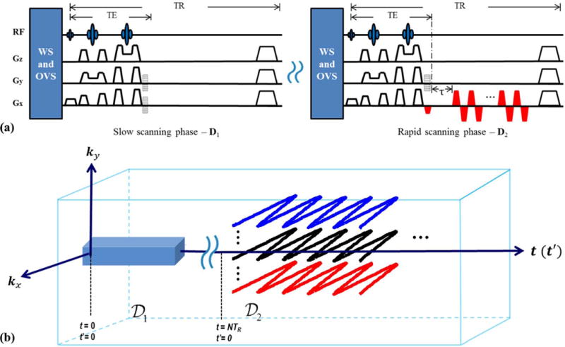
The proposed SPICE sequence for 2D¹H-MRSI: (a) the hybrid CSI/EPSI sequence with the CSI component (left) to acquire ${\mathcal{D}}_1$ and the EPSI-like component (right) to acquire ${\mathcal{D}}_2$; (b) the (k,t)-space trajectories generated by the sequence in (a). See the text for more detailed description of the sequence.

While the proposed hybrid CSI/EPSI sequence can be readily extended to 3D by adding additional phase encodings along the third spatial dimension, it may be too slow to provide the desired number of spatiospectral encodings for practical high-resolution 3D¹H-MRSI (e.g., acquiring 12 × 12 × 12 spatial encodings using a 3D CSI for ${\mathcal{D}}_1$ alone would take about 30 minutes with TR= 1 s). To address this problem, we propose a dual-density, dual-speed EPSI sequence to further accelerate the spatiospectral encoding for 3D MRSI using SPICE. More specifically, for the acquisition of ${\mathcal{D}}_1$, we replace the CSI component with a slow 3D EPSI scan (with a lower readout bandwidth) that covers a limited region of k-space and has full spectral encoding (Fig. 3a, left column). Moreover, this 3D EPSI scan has two-dimensional phase encodings, making the acquisition time for ${\mathcal{D}}_1$ equivalent to the CSI encoding in the 2D SPICE sequence. For the acquisition of ${\mathcal{D}}_2$, we can further reduce the data acquisition time by performing a rapid EPSI scan (Fig. 3a, right column) that simultaneously encodes two spatial dimensions (e.g., x and y) as well as the spectral dimension during each FID. The third spatial dimension (e.g., z) is phase encoded, and multiple echo shifts are used to obtain additional spectral encodings. The resulting (k,t)-space trajectories for such a 3D sequence are shown in Fig. 3b. As can be seen, the entire (k_y, k_x) plane is traversed by each echo shift in ${\mathcal{D}}_2$, providing many spatial encodings after each excitation.

Figure 3.

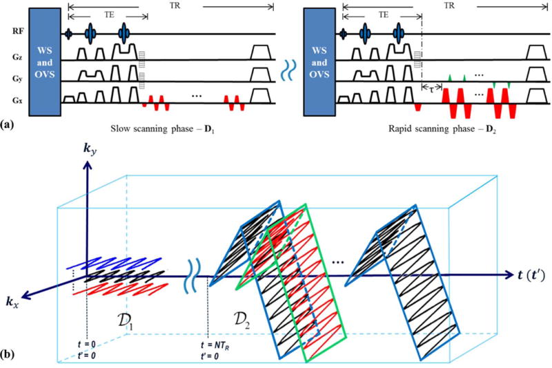
The proposed SPICE sequence for 3D¹H-MRSI: (a) the dual-density, dual-speed EPSI sequence with the slow EPSI component (left) to acquire ${\mathcal{D}}_1$ and the rapid EPSI component to acquire ${\mathcal{D}}_2$. τ denotes the timing for the echo shifts that can be used for additional spectral encodings; (b) the corresponding (k,t)-space trajectories generated by the sequence in (a).

Image Reconstruction

The measured (k,t)-space MRSI data can be expressed as

$$s_c\left(\mathbf{k},t\right)={\displaystyle \underset{V}{\int }\left({\rho }_m\left(\mathbf{r},t\right)+{\rho }_{ns}\left(\mathbf{r},t\right)\right)S_c}\left(\mathbf{r}\right)e^{-i\gamma \mathrm{\Delta }B\left(\mathbf{r}\right)t}{e}^{-i2\pi \mathbf{k}\mathbf{r}}d\mathbf{r}+\xi \left(\mathbf{k},t\right),$$ [2]

where V is the excited volume, γ the gyromagnetic ratio, S_c(r) the sensitivity profile of the c^th coil, ∆B (r) the B₀ field inhomogeneity map (assumed to be readily available from an auxiliary scan), ξ (k; t) contains the measurement noise (modeled as complex white Gaussian), ρ_m (r, t) represents the metabolite signal of interest and ρ_ns (r, t) the residual nuisance signal components, i.e., the residual water, subcutaneous fat and baseline signals for¹H-MRSI of the brain. Accordingly, a discretized data model can be used as

$${\mathrm{s}}_c=\mathrm{\Omega }\left\{\mathrm{F}\left[\mathrm{B}\odot \left({\mathit{\rho }}_{c,m}+{\mathit{\rho }}_{c,ns}\right)\right]\right\}+{\mathit{\xi }}_c$$ [3]

where s_c is a vector containing the data for the c^th coil, Ω a (k,t)-space sampling operator, F a Fourier transform matrix, B a phase term modeling the field inhomogeneity effects as described in Eq. [2] $\left(\text{with}{\mathrm{B}}_{nm}=e^{-i\mathrm{\gamma }\mathrm{\Delta }B\left({\mathbf{r}}_n\right)t_m}\right)$, ⊙ denotes entry-wise multiplication, ρ_c,m and ρ_c,ns are matrix representations of ρ_m (r, t) S_c (r) and ρ_ns (r, t) S_c (r), and ξ_c the noise vector. In the following discussions, for notational convenience, we assume a uniform sensitivity profile (i.e., S_c(r) = 1) and drop the coil index.¹

For image reconstruction from ${\mathcal{D}}_1$ $\left(\text{expressed}\text{as}{\mathcal{D}}_1={\left\{d_1\left({\mathbf{k}}_n,t_m\right)\right\}}_{n,m=1}^{N_1,M_1}\right)$ and ${\mathcal{D}}_2$ (expressed as ${\mathcal{D}}_2={\left\{d_2\right({\widehat{\mathbf{k}}}_n,{\widehat{t}}_m\left)\right\}}_{n,m=1}^{N_2,M_2}$), we incorporate low-rank models on ρ_m and ρ_ns (based on the PS representation in Eq. [1]) and use the following imaging equation (26,27,30)

$$\mathbf{s}=\mathrm{\Omega }\left\{\mathbf{F}\left[\mathbf{B}\odot \left({\mathbf{C}}_m{\mathbf{\Phi }}_m+{\mathbf{C}}_{ns}{\mathbf{\Phi }}_{ns}\right)\right]\right\}+\mathit{\xi },$$ [4]

where ${\mathbf{C}}_m\in {ℂ}^{N_2\times L_1}$, ${\mathbf{C}}_{ns}\in {ℂ}^{N_2\times L_2}$, ${\mathbf{\Phi }}_m\in {ℂ}^{L_1\times M_1}$ and ${\mathbf{\Phi }}_{ns}\in {ℂ}^{L_2\times M_1}$ are low-rank matrices (L₁, L₂ < min {N₂; M₁}). If the contribution of the nuisance signals is negligible (or removed from the data in preprocessing (29)), we can let C_ns Φ_ns = 0. Otherwise, this component can be included to capture the remaining nuisance signals. According to Eq. [4], SPICE defines the reconstruction problem as determining Φ = [Φ_m; Φ_ns] and C = [C_m, C_ns].

Subspace Estimation

According to Eqs. [3] and [4], Φ can be easily estimated from ${\mathcal{D}}_1$ (e.g., through singular value decomposition (26, 27)) in the absence of field inhomogeneity. In the presence of non-negligible field inhomogeneity, as it is the case for in vivo experiments, its effects need to be removed (28). The challenge in solving this problem lies in the limited data available in ${\mathcal{D}}_1$ (33). We propose to obtain a field inhomogeneity corrected ${\widehat{\mathit{\rho }}}_1$ by solving the following regularized reconstruction problem using a coil-combined ${\mathcal{D}}_1$, denoted by a vector ${\mathrm{d}}_1\in {ℂ}^{N_1{M}_1\times 1}$,

$${\widehat{\mathit{\rho }}}_1=\text{arg}\underset{\rho }{\min }{\Vert {\mathbf{d}}_1-{\mathrm{\Omega }}_1\left\{\mathbf{F}\left(\mathbf{B}\odot \mathit{\rho }\right)\right\}\Vert }_2^2+\mathrm{\lambda }{\Vert \mathit{\rho }\Vert }_{\ast },$$ [5]

where ${\widehat{\mathit{\rho }}}_1$ has a size of ${\widehat{N}}_1\times M_1$ (with ${\widehat{N}}_1$ matching the grid size of the field map to ensure accurate field inhomogeneity modeling (33)), Ω₁ is a sampling operator for data in ${\mathcal{D}}_1$, and F and B the same as described in Eq. [3]. The regularization term ∥·∥_* is the nuclear-norm penalty (34) and λ is the regularization parameter. While other choices for the regularization term can be used, the low-rankness encouraging nuclear-norm penalty is well motivated by the low-dimensional subspace model of the underlying ρ. We solve Eq. [5] using the augmented Lagrange multiplier method described in (35). After ${\widehat{\mathit{\rho }}}_1$ is obtained, it is rearranged into a Casorati matrix to which a singular value decomposition (SVD) can be applied. The first L right singular vectors are then chosen to form the matrix Φ. The model order L is selected based on examining the singular value decay of the Casorati matrix. For further separation of the subspaces for metabolite and nuisance signals, i.e., Φ_m and Φ_ns, please refer to (29).

Estimation of Spatial Coefficients

Given the estimated subspace, the model in Eq. [4] can be further specified as

$${\mathbf{d}}_2={\mathrm{\Omega }}_2\left\{\mathbf{F}\left[\mathbf{B}\odot \left({\mathbf{C}}_m{\mathbf{\Phi }}_m+{\mathbf{C}}_{ns}{\mathbf{\Phi }}_{ns}\right)\right]\right\}+{\mathit{\xi }}_2$$ [6]

where ${\mathrm{d}}_2\in {ℂ}^{N_2{M}_2\times 1}$ denotes the vector containing data from ${\mathcal{D}}_2$, Ω₂ the sparse sampling operator for data in ${\mathcal{D}}_2$, and ξ₂ the noise vector. Accordingly, image reconstruction can be done by estimating C_m and C_ns, which can be formulated into the following regularized least-squares problem

$$\begin{array}{l}{\widehat{\mathbf{C}}}_m,{\widehat{\mathbf{C}}}_{ns}=\text{arg}\underset{{\mathbf{C}}_m,{\mathbf{C}}_{ns}}{\min }{\Vert {\mathbf{d}}_2-{\mathrm{\Omega }}_2\left\{\mathbf{F}\left[\mathbf{B}\odot \left({\mathbf{C}}_m{\mathbf{\Phi }}_m+{\mathbf{C}}_{ns}{\mathbf{\Phi }}_{ns}\right)\right]\right\}\Vert }_2^2\\ +{\mathrm{\lambda }}_1{\mathrm{\Psi }}_1\left({\mathbf{C}}_m,{\mathbf{\Phi }}_m\right)+{\mathrm{\lambda }}_2{\mathrm{\Psi }}_2\left({\mathbf{C}}_{ns},{\mathbf{\Phi }}_{ns}\right),\end{array}$$ [7]

where ${\Vert \cdot \Vert }_2^2$ measures the data consistency and Ψ₁(·) and Ψ₁(·) represent the regularization functionals for metabolite and nuisance signals, respectively, with regularization parameters λ₁ and λ₂. Many choices can be made for Ψ_1,2(·) to incorporate prior information about the unknown spatiospectral/spatiotemporal function (e.g., those in (19, 23)). In this work, we choose the following regularization form for the metabolite signal component

$${\mathrm{\Psi }}_1\left({\mathbf{C}}_m,{\mathbf{\Phi }}_m\right)={\Vert \mathbf{W}\mathbf{D}{\mathbf{C}}_m{\mathbf{\Phi }}_m\mathbf{\Psi }\Vert }_1,$$ [8]

where D is a finite difference operator, W contains edge weights derived from high-resolution anatomical images (17) and Ψ denotes a temporal sparsifying transform (e.g., the Fourier transform for MRSI (24)). This choice is motivated by the advantages of such edge-preserving (or non-quadratic) penalties shown in recent developments for sparse sampling and denoising. Similar forms of regularization can also be found in the context of dynamic imaging (36–39). For the nuisance signal component, an ℓ₂ regularization was used as in (29) for better conditioning and faster computation, although more sophisticated schemes can also be considered in the future. A number of efficient algorithms can be used to solve the problem in Eq. [7] with the non-quadratic regularization in Eq. [8]. Here, we use a variable splitting reformulation and an alternating direction method of multipliers (ADMM) based algorithm. Further description of this algorithm can be found in the appendix.

METHODS

Practical Implementations

Sampling Consideration

Given a subspace with dimension L, the number of spatial encodings in ${\mathcal{D}}_1$ (i.e., N₁) theoretically has at least to be greater than L. This is easy to satisfy since L is typically a small number with the field inhomogeneity effects removed (26,28). In practice, however, a sufficiently large N₁ is needed for effective field inhomogeneity correction and nuisance signal removal. Based on our experience in simulation and experimental studies, an N₁ greater than 12 × 12 for 2D and 12 × 12 × 12 for 3D provides a good tradeoff between acquisition time and the performance of field inhomogeneity correction and nuisance signal removal (29,33). Meanwhile, the number of echoes (or echo shifts) acquired for ${\mathcal{D}}_2$ typically ranges from 4L to 6L in order to provide reasonable conditioning for the spatial coefficient fitting problem.

Echo Inconsistency Correction

For maximizing encoding efficiency, we have incorporated the capability of acquiring data on both polarities of the gradients into the SPICE sequences. To make use of all the data, the inconsistency between echoes acquired on positive and negative gradients (referred to as “odd” and “even” echoes) need to be corrected (9). To this end, two navigator echo trains with reversed x-gradients (without phase encoding and water suppression) were acquired preceding the actual EPSI encoding. With these data, the k-space center misalignments (∆k) were first estimated from each pair of positive and negative gradients and the averaged ∆k was then used to correct the misalignment between odd and even echoes in the actual EPSI encodings. In addition, a phase correction term was estimated from the aligned echoes of the navigators and applied to the even echoes in the EPSI encodings. The advantages of using such navigators for echo correction are: 1) since no water suppression is applied, the estimated correction parameters will have high fidelity due to the high SNR of the water signals; and 2) the phase differences estimated from the time-matched gradients from the navigators do not include chemical-shift-induced phase differences thus only reflects the effects of the gradients.

Nuisance Signal Removal and Multi-Coil Processing

For¹H-MRSI of the brain, the strong nuisance water and subcutaneous fat signals need to be removed for the SPICE reconstruction. To this end, a recently proposed subspace-based nuisance signal removal method is included in the data processing (29). Since multiple coils are used for acquisition, the removal is applied coil by coil to both ${\mathcal{D}}_1$ and ${\mathcal{D}}_2$. Afterwards, the nuisance signal removed ${\mathcal{D}}_1$ data are combined using an SVD-based scheme (40) for subsequent field inhomogeneity correction and subspace estimation. After the subspace is estimated, a spline-based interpolation is applied to the temporal basis functions (rows of Φ) to match the temporal sampling grids of ${\mathcal{D}}_2$ for spatial coefficient estimation, which is also performed in a coil-by-coil fashion followed by an SVD-based combination to form the final spatiotemporal reconstruction. All the regularization parameters were selected using the discrepancy principle (43). A flow chart summarizing the entire data processing pipeline for¹H-MRSI of the brain using SPICE is shown in Figure S1 (Supporting Materials).

Experimental Studies

Experimental¹H-MRSI data from both a physical phantom and healthy volunteers have been acquired to evaluate the performance of the proposed method (also referred to as SPICE hereafter) and demonstrate its feasibility for obtaining high-resolution¹H metabolite distributions from the brain. All experiments were performed on a Siemens Trio 3T scanner (Siemens Medical Solutions, Erlangen, Germany) equipped with a 12-channel receiver headcoil.

Phantom Experiments

A customized brain metabolite phantom was built using a cylindrical jar (made with polymethylpentene) filled with NaCl-doped water and three rows of vials with different diameters to demonstrate the resolution capability of the SPICE. The vials contained solutions of N-acetylaspartate (NAA), creatine (Cr), choline (Cho), and myo-inositol (mI) with physiologically relevant concentrations (41). The design of the phantom is illustrated in Fig. 4a. More specifically, the bottom row (vials with the largest diameter) contains approximately 20 mmol/L NAA, 15 mmol/L Cr, 5 mmol/L Cho and 10 mmol/L mI. The middle row contains approximately 10 mmol/L NAA, 10 mmol/L Cr, 5 mmol/L Cho and 10 mmol/L mI. The top row (vials with the smallest diameter) contains approximately 15 mmol/L NAA, 10 mmol/L Cr, 5 mmol/L Cho and 10 mmol/L mI.

Figure 4.

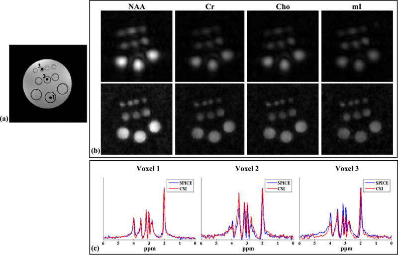
Experimental results from the metabolite phantom obtained by a 24 × 24 CSI and an 80 × 80 SPICE with equivalent data acquisition time. The GRE image in (a) shows the structural arrangement of the phantom. The images in (b) compare the spatial maps (obtained by peak integral) of NAA (first column), Cr (second column), Cho (third column) and mI (fourth column) for CSI (top row) and SPICE (bottom row). The NAA maps were normalized such that the maximum intensity is 1 (for both CSI and SPICE), while the other metabolite maps were normalized to the NAA maps. All reconstructions were zero-filled to 110 × 110 grids. The images in (c) show spectra from the three numbered voxels indicated in (a) for CSI (red) and SPICE (blue). Each spectrum was normalized to its maximum value individually.

Data from this phantom were acquired using the proposed 2D SPICE sequence. The 2D acquisition was performed with 12 × 12 spatial encodings in ${\mathcal{D}}_1$, each having 512 temporal samples, and 80 × 80 spatial encodings in ${\mathcal{D}}_2$, each having 128 echoes. Six averages were acquired for ${\mathcal{D}}_2$ (with a factor of 9/10 partial Fourier sampling), making the total acquisition time 9.7 minutes. An equivalent-time standard CSI acquisition with 24 × 24 spatial encodings was performed. The other relevant imaging parameters were (for both acquisitions): FOV=220 × 220 mm², volume of excitation (VOX)=160 × 160 × 10 mm³, TR/TE=1000/30 ms, WET water suppression BW=80 Hz (water suppression enhanced through T1 effects, see (42) for details), and delta frequency (for PRESS excitation)=−2.4 ppm (water at 0 ppm). The sampling BWs for the CSI and EPSI scans were 2 kHz and 100 kHz, respectively. A high-resolution 2D GRE image (with a matrix size of 192 × 192) and a 2D ∆B₀ map (with a matrix size of 110 × 110) were acquired for extracting edge information and performing field inhomogeneity correction. These images were co-registered to the spectroscopic data and had the same FOV and slice thickness.

For 3D acquisitions, ${\mathcal{D}}_1$ contained 12 × 12 × 12 (k_x-k_y-k_z) spatial encodings each with 512 echoes. The spectral BW was approximately 1700 Hz. ${\mathcal{D}}_2$ contained 48 echo shifts (uniformly spaced by 1.57 ms) each with 72 × 72 × 20 spatial encodings. Other imaging parameters were: FOV=220 × 220 × 72 mm³, VOX=160 × 160 × 56 mm³, TR/TE=1000/30ms, and water suppression BW=80 Hz. The sampling BWs for the slow and rapid EPSI scans were 60 kHz and 100 kHz, respectively. The total acquisition time was 18.5 minutes. Co-registered multi-slice GRE images and ∆B₀ maps with a matrix size of 110 × 110 × 36 and matched FOV (isotropic 2 mm resolution) were also acquired.

In Vivo Experiments

Human brain¹H-MRSI data were acquired with the approval of the Institutional Review Board at the University of Illinois and the written consent of the participants. For in vivo experiments, a 3D, T₁-weighted structural scan (MPRAGE, 0.9×0.9×1.0 mm³ voxel size) was first performed for localizing the MRSI slice/volume and for extracting anatomical information used in data processing, e.g., segmented water and fat images for nuisance signal removal (29) and edge structures for reconstruction.

For 2D acquisitions, 12 × 12 spatial encodings each with 512 temporal samples (for ${\mathcal{D}}_1$) and 80 × 80 spatial encodings each with 128 echoes (for ${\mathcal{D}}_2$) were acquired. Four signal averages were used for ${\mathcal{D}}_2$, making the total acquisition time 10 minutes. The rest of the imaging parameters were: FOV=220 × 220 mm², VOX=150 × 160 × 8 mm³, TR/TE=1300/30 ms and water suppression BW=80 Hz. Eight outer volume suppression (OVS) slabs were included for lipid suppression. The sampling BWs for the CSI and EPSI scans were 2 kHz and 100 kHz. Moreover, as in phantom experiments, a ∆B₀ map was acquired for field inhomogeneity modeling and correction (with matched FOV and slice thickness, and a matrix size of 110 × 110). To further demonstrate the capability of SPICE in achieving a combination of high resolution and high SNR, equivalent-time CSI and conventional EPSI scans were also performed for comparison. In the same data acquisition time (10 min), the CSI acquisition generated 22 × 22 spatial encodings while the EPSI acquisition had 80 × 80 spatial encodings with three averages and two temporal interleaves (to satisfy the spectral Nyquist criterion). The other imaging parameters remained the same.

For 3D¹H-MRSI experiments on the brain, the proposed data acquisitions contained 16 × 16 × 16 spatial encodings each with 512 echoes in ${\mathcal{D}}_1$ (spectral BW≈1500 Hz) and 80 × 80 × 20 spatial encodings in ${\mathcal{D}}_2$ each with 120 echoes. The other important imaging parameters were: FOV=240 × 240 × 72 mm³, VOX=240 × 240 × 64 mm³, TR/TE=1100/20ms, water suppression BW=80 Hz and number of OVS slabs=8. The sampling BWs for the slow and rapid EPSI scans were 68 kHz and 125 kHz, respectively. The total acquisition time was 25.5 minutes. For field inhomogeneity correction, multi-slice ∆B₀ maps were acquired (with matched FOV and a matrix size of 120 × 120 × 36, i.e., 2 mm isotropic resolution). The MPRAGE image was registered to the field maps for obtaining structural information needed for processing and reconstruction.

RESULTS

Phantom Experiments

Figures 4 and 5 present representative results from the 2D phantom studies. The CSI reconstruction was obtained using a field inhomogeneity corrected conjugate phase (CP) reconstruction (33, 44). The SPICE reconstruction was obtained using a model order L = 6. Figure 4b compares the spatial distributions of NAA, Cr, Cho and mI from CSI and SPICE. The spatial distributions were obtained by integrating around the strongest peaks for each metabolite. As can be seen, the CSI reconstruction has high SNR but suffers from serious blurring and ringing artifacts (due to the truncation in k-space). With the same data acquisition time, SPICE achieves high spatial resolution while maintaining very good SNR. Particularly, the vials at the first and second rows (with the smallest and medium sizes) are severely blurred in the CSI reconstruction, while even the smallest vials can be distinguished in the SPICE reconstruction (e.g., the center two which are merged together in the CSI). Figure 4c shows spectra from both CSI and SPICE corresponding to voxels selected from each row of the vials (the voxel locations are indicated in Fig. 4a). SPICE produces high-quality spectra with a similar SNR compared to those from CSI.

Figure 5.

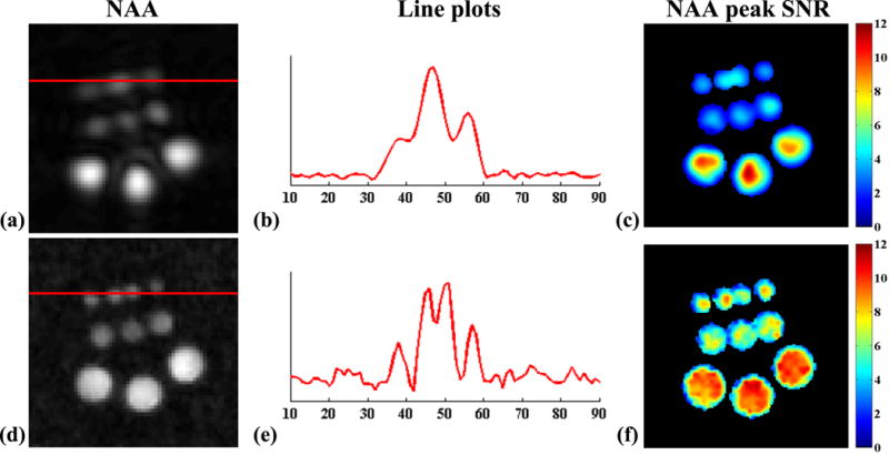
Results from the equivalent-time acquisitions on the phantom (10 min) obtained by CSI (top row) and SPICE (bottom row). Left column: NAA maps (as shown in Fig. 4); middle column: 1D plots corresponding to the red lines in the NAA maps; right column: peak SNR maps for NAA.

The resolution and SNR capability of SPICE is further demonstrated in Fig. 5. The line plots clearly show that SPICE was able to spatially resolve the smallest vials (Fig. 5e) while CSI cannot (Fig. 5b). The peak SNR maps for NAA (Fig. 5c and f) show that the SPICE reconstruction has similar SNR to the low-resolution CSI but the SNR distribution for SPICE is more uniform due to higher spatial resolution and the effects of regularization. Note that the peak SNR for NAA was calculated as

$${\text{SNR}}_{\text{NAA}}=\frac{\sqrt{{\displaystyle {\sum }_{\mathrm{p}\in {\omega }_{\text{NAA}}}{\left|\rho \right(\mathbf{r},{\mathrm{f}}_{\mathrm{p}}\left)\right|}^2}}}{\left|{\omega }_{\text{NAA}}\right|{\sigma }_{\mathrm{f}}},$$

where ω_NAA contains the frequency indices for the strongest NAA peak centered at 2.02 ppm, |ω_NAA| denotes the cardinality of ω_NAA, and σ_f denotes the noise standard deviation in the spectral domain. The range of ω_NAA was chosen as 0.2 ppm for our experiments. σ_f was estimated from a spectral region with negligible metabolite spectral components.

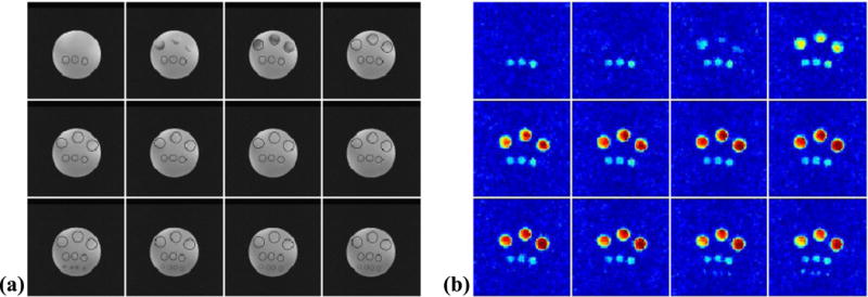
Figure 6 shows a set of representative results from 3D phantom experiments. The SPICE reconstruction was obtained using a model order L = 12. The reconstruction was then zero-filled to a matrix size of 100 × 100 × 24 for visualization. The spatial maps of NAA for different slices obtained by spectral integration are shown in Fig. 6b. As can be seen, 3D SPICE achieved simultaneously very high spatial resolution and high SNR, clearly resolving the smallest vials and cross-slice variations in the NAA distribution.

Figure 6.

A set of representative 3D phantom results obtained by the proposed method: (a) the center 12 slices from the GRE image of the phantom; (b) the NAA maps for the corresponding slices.

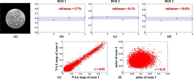
Figure 7 demonstrates the reproducibility of SPICE. In this experiment, four 3D SPICE data sets were repeatedly acquired with the same imaging parameters. The GRE image was acquired only once while the field mapping scan was repeated for each 3D acquisition. SPICE reconstructions were generated from each data set with the same reconstruction parameters. As shown by the mean intensities of NAA in three regions of interest (3×3 blocks selected from one vial in each row) and the plot of NAA intensities obtained from scan 1 versus those from scan 4, SPICE achieved very high repeatability (with coefficients of variation less than 10%, Fig. 7b–d) even at this high spatial resolution. Moreover, the NAA maps from different scans are highly correlated (e.g., the correlation coefficient for scans 1 and 4 is 0.92, Fig. 7e) while the noise samples (from background regions) show negligible correlation (Fig. 7f). This implies that the strong correlation in the estimated metabolite distributions does not come from a strong systematic bias introduced by the model or the regularization.

Figure 7.

Reproducibility results for SPICE from 3D phantom experiments: (a) a GRE image indicating the three regions of interest (ROIs) for analysis; (b)–(d) mean intensities of NAA from the three ROIs for the four repeated scans (described in the text); (e) the plot of NAA intensities for scan 1 against scan 4; and (f) the plot of noise samples from scan 1 against scan 4. The solid lines in (b)–(d) stand for the mean of the four scans and the dash lines represent the standard deviation (std).

In Vivo Experiments

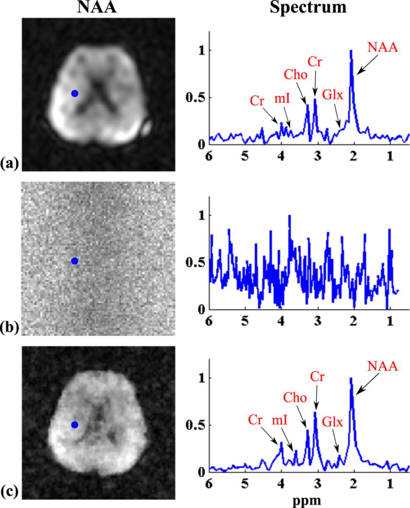
Figure 8 compares the results from the equivalent-time in vivo 2D experiment (10 min). The spatial maps of NAA obtained by CSI, EPSI and SPICE (all having the same data acquisition time) are compared along with representative spectra. The CSI and EPSI reconstructions were obtained by the CP method, while the SPICE reconstruction was obtained with a model order L = 8. All reconstructions were then zero-filled to a matrix size of 128 × 128. As can be seen, SPICE yields similar SNR but significantly higher resolution than CSI, which again suffers from severe truncation artifacts. Compared to the equivalent-time high-resolution EPSI acquisition which produced very noisy spatiospectral distribution, SPICE yields dramatic improvement in SNR. It is worth noting that although concealed by noise, the high-resolution EPSI data contained the metabolite signals of interest.² The capability to recover these signals with a predetermined subspace structure from the high SNR ${\mathcal{D}}_1$ is a unique property of SPICE.

Figure 8.

2D¹H-MRSI of the brain from three equivalent-time acquisitions (10 min): (a) a 22 × 22 CSI; (b) an 80 × 80 EPSI; and (c) a SPICE acquisition with 12 × 12 spatial encodings in ${\mathcal{D}}_1$ and 80 × 80 spatial encodings in ${\mathcal{D}}_2$. The left column shows NAA maps from the three acquisitions and the right column plots representative spectra from the voxels identified by the blue dots in the NAA maps.

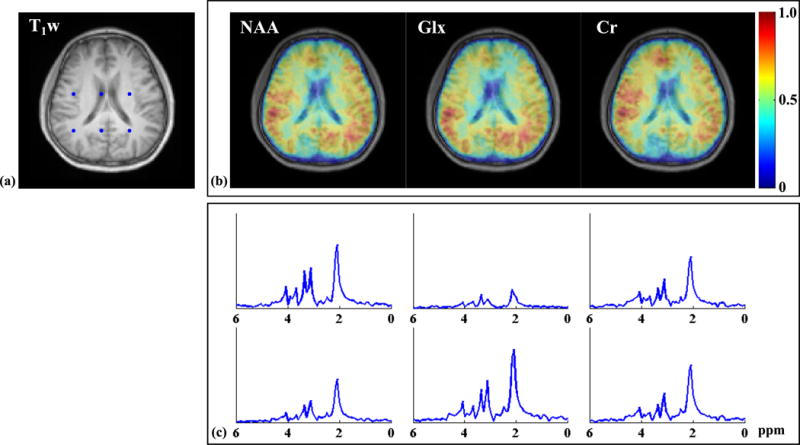
The spatial maps of NAA, Glx (glutamine+glutamate), and Cr obtained from another 2D SPICE acquisition are also shown in Fig. 9b along with representative spectra in Fig. 9c. As is clear from the images, SPICE reveals local variations of the metabolite distributions that appear to have good correspondence with anatomical structures. Additionally, the spectra from SPICE reconstruction again show very high quality. Further validation is needed to confirm these observations.

Figure 9.

Results from a 10 min 2D-SPICE acquisition: (a) the T₁-weighted image (T₁w); (b) the spatial maps of different metabolites (NAA, Glx and Cr) produced by the SPICE reconstruction corresponding to the same slice (as in a); (c) representative spectra selected from the voxels indicated by the blue dots in (a). The metabolite maps were normalized individually, color-coded and overlaid on the T₁-weighted image.

Figure 10 shows a set of 3D in vivo results. The spatial maps of NAA for six different slices (Fig. 10b) and representative spectra from two different voxels (Fig. 10c–d) are shown. As can be seen, the SPICE reconstruction shows high SNR and is able to resolve cross-slice differences in metabolite distributions. The reconstructed spectrum also shows high SNR, while the quality may be further improved by optimizing the k-t space trajectories and acquisition parameters. The intensity variations between the anterior and posterior parts of the brain could be due to remaining coil sensitivity effects. The placement of OVS bands can be another contributing factor for the observed variations (especially at the edge of the brain), which can be removed with the availability of more advanced lipid suppression/removal methods.

Figure 10.

Results from a 3D SPICE acquisition: (a) the T₁-weighted images (from the MPRAGE scan) resized to the grids of the SPICE reconstruction; (b) spatial maps of NAA for the corresponding six slices shown in (a); (c)–(d) spectra from the voxels at the red and blue dots.

DISCUSSION

We have demonstrated the capability of the proposed method in achieving¹H-MRSI of the brain with high spatial resolution and high SNR in practical experiments. This section discusses several relevant issues worth of further research for enhancing the performance and practical utility of the proposed method.

First, the proposed sequences described in this paper used PRESS for excitation, which can be subject to chemical shift displacement and limited in the range of echo times (41). Therefore, further optimizations of the pulse sequences are desirable and currently being investigated. They include incorporating LASER-type of pulses (45,46) to reduce chemical shift displacement errors for improved spatial localization, and developing spin-echo and FID acquisitions to achieve shorter echo times (8,47) for improved SNR and detection of short-T₂ and J-coupled metabolites.

Second, the multi-coil acquisition is mainly used for improving SNR in our current implementations (through the SVD-based coil combination). However, integration of parallel imaging, which has been shown useful in various MRSI studies (10), into the current SPICE acquisition and reconstruction framework can provide additional flexibility in trading off speed, SNR and resolution (10,13–15), making SPICE more adaptive to various practical applications. More specifically, if sufficient SNR is available (e.g., for 3D or lower resolution acquisitions), the parallel imaging capability can be used for further acceleration. If the SNR is limited, it can still allow us to design a scheme to optimally combine the data from multiple coils without further spatial undersampling.

Another important problem for future research is the optimization of the (k,t)-space sampling strategy and reconstruction scheme, especially for 3D SPICE (with parallel imaging). For example, in order to achieve high-resolution 3D¹H-MRSI of the brain in a shorter time frame, the capability to further accelerate the SPICE acquisition by integrating compressed sensing-based sparse sampling can be explored. Furthermore, the (k,t)-space trajectories can also be optimized for improved spatiospectral encoding efficiency (through both theoretical analysis and experimental studies). Building on these optimizations, we can also improve the reconstruction method. For example, stronger spatiospectral/spatiotemporal prior information and/or better sparsity constraints can be exploited. Other potential extensions also include utilizing data from both ${\mathcal{D}}_1$ and ${\mathcal{D}}_2$ for improved spatial coefficient estimation and jointly determining the subspace structure and spatial coefficients from the hybrid data sets.

CONCLUSIONS

Special data acquisition and reconstruction methods have been developed to enable high-resolution¹H-MRSI of the brain based on the recently proposed SPICE spectroscopic imaging framework. Experimental studies have been performed on phantom and human subjects to evaluate the performance of the proposed methods. These studies demonstrate that SPICE provides a significantly better tradeoff for resolution, SNR and speed, and achieves very good reproducibility in metabolite phantom experiments. For in vivo 2D MRSI, SPICE is able to produce high-SNR spatiospectral distributions with an approximately 3 mm nominal in-plane resolution from a 10-min acquisition. For 3D MRSI, SPICE is able to achieve an approximately 3 mm in-plane and 4 mm through-plane resolution in about 25 min. With further optimizations in signal excitation, data acquisition and image reconstruction, SPICE can be a useful tool for in vivo metabolic studies of the brain.

Supplementary Material

Supp FigureS1

Figure S1: Data processing pipeline for ¹H-MRSI of the brain using SPICE. The lower case letter c denotes the coil index. ${d^{\prime }}_{1,c}(\cdot )$ and ${d^{\prime }}_{2,c}(\cdot )$ denote the water-fat removed ${\mathcal{D}}_1$ and ${\mathcal{D}}_2$ for all the coils. The variables without the coil index denote the data after coil combination.

APPENDIX

The ADMM algorithm

We introduce the following variable splitting reformulation for Eq. [7] with the non-quadratic regularization in Eq. [8]

$$\begin{array}{l}\widehat{\mathbf{C}},\widehat{\mathbf{P}},\widehat{\mathbf{Q}}=\text{arg}\underset{\mathbf{C},\mathbf{P},\mathbf{Q}}{\min }{\Vert {\mathbf{d}}_2-{\mathrm{\Omega }}_2\left\{\mathbf{F}\mathbf{P}\right\}\Vert }_2^2+{\mathrm{\lambda }}_1{\Vert \mathbf{Q}\Vert }_1+{\mathrm{\lambda }}_2{\Vert {\mathbf{C}}_{ns}\Vert }_F^2\\ s.t.\mathbf{P}=\mathbf{B}\odot \left(\mathbf{C}\mathbf{\Phi }\right)\\ \mathbf{Q}={\mathbf{D}}_w{\mathbf{C}}_m{\mathbf{\Phi }}_m\mathbf{\Psi }\end{array}$$ [9]

with auxiliary variables P and Q and D_w = WD. The variable C contains both C_m and C_ns and Φ contains both Φ_m and Φ_ns. Note that by introducing P, we separate the Fourier encoding operator and the field inhomogeneity operator which can significantly simplify the computations associated with both of them (similar approaches have been used in several parallel imaging reconstruction literature to separate Fourier and sensitivity encoding operators, e.g., (48)). An ADMM based (49, 50) algorithm is used to solve the problem in Eq. [9]. More specifically, the algorithm iterates between minimizing the following augmented Lagrangian function

$$\begin{array}{l}ℒ(\mathbf{C},\mathbf{P},\mathbf{Q},{\mathbf{Y}}^{(i)},{\mathbf{Z}}^{\left(i\right)})={\Vert {\mathbf{d}}_2-{\mathrm{\Omega }}_2\left\{\mathbf{\text{FP}}\right\}\Vert }_2^2+{\mathrm{\lambda }}_1{\Vert \mathbf{Q}\Vert }_1+\frac{{\mu }_1}{2}{\Vert \mathbf{P}-\mathbf{B}\odot \left(\mathbf{C}\mathbf{\Phi }\right)\Vert }_F^2+\langle {\mathbf{Y}}^{(i)},\mathbf{P}-\mathbf{B}\odot \left(\mathbf{C}\mathbf{\Phi }\right)\rangle \\ +\frac{{\mu }_2}{2}{\Vert \mathbf{Q}-{\mathbf{D}}_w{\mathbf{C}}_m{\mathbf{\Phi }}_m\mathbf{\Psi }\Vert }_F^2+\langle {\mathbf{Z}}^{(i)},\mathbf{Q}-{\mathbf{D}}_w{\mathbf{C}}_m{\mathbf{\Phi }}_m\mathbf{\Psi }\rangle +{\mathrm{\lambda }}_2{\Vert {\mathbf{C}}_{ns}\Vert }_F^2,\end{array}$$ [10]

with respect to C, P, and Q alternatively, and updating the Lagrangian multipliers Y and Z as

$$\begin{array}{l}{\mathbf{Y}}^{(i+1)}={\mathbf{Y}}^{(i)}+{\mu }_1\left({\mathbf{P}}^{(i)}-\mathbf{B}\odot \left({\mathbf{C}}^{(i)}\mathbf{\Phi }\right)\right)\\ {\mathbf{Z}}^{(i+1)}={\mathbf{Z}}^{(i)}+{\mu }_2\left({\mathbf{Q}}^{(i)}-{\mathbf{D}}_w{\mathbf{C}}_m^{(i)}{\mathbf{\Phi }}_m\mathbf{\Psi }\right).\end{array}$$

μ₁ and μ₂ are pre-selected penalty parameters. The operation ⟨·,·⟩ denotes the inner product. Each resulting subproblem can be easily derived. Detailed iterative procedures are not shown here but similar derivations can be found in Refs. (48–50).

References

- 1.Mansfield P. Spatial mapping of the chemical shift in NMR. Magn Reson Med. 1984;1:370–386. doi: 10.1002/mrm.1910010308. [DOI] [PubMed] [Google Scholar]
- 2.Posse S, Tedeschi G, Risinger R, Ogg R, Le Bihan D. High speed 1H spectroscopic imaging in human brain by echo planar spatial-spectral encoding. Magn Reson Med. 1995;33:34–40. doi: 10.1002/mrm.1910330106. [DOI] [PubMed] [Google Scholar]
- 3.Pohmann R, von Kienlin M, Haase A. Theoretical evaluation and comparison of fast chemical shift imaging methods. J Magn Reson. 1997;129:145–160. doi: 10.1006/jmre.1997.1245. [DOI] [PubMed] [Google Scholar]
- 4.Adalsteinsson E, Irarrazabal P, Topp S, Meyer C, Macovski A, Spielman DM. Volumetric spectroscopic imaging with spiral-based k-space trajectories. Magn Reson Med. 1998;39:889–898. doi: 10.1002/mrm.1910390606. [DOI] [PubMed] [Google Scholar]
- 5.Guimaraes AR, Baker JR, Jenkins BG, Lee PL, Weisskoff RM, Rosen BR, Gonzalez RG. Echoplanar chemical shift imaging. Magn Reson Med. 1999;41:877–882. doi: 10.1002/(sici)1522-2594(199905)41:5<877::aid-mrm4>3.0.co;2-3. [DOI] [PubMed] [Google Scholar]
- 6.Schirda CV, Tanase C, Boada FE. Rosette spectroscopic imaging: Optimal parameters for alias-free, high sensitivity spectroscopic imaging. J Magn Reson Imag. 2009;29:1375–1385. doi: 10.1002/jmri.21760. [DOI] [PubMed] [Google Scholar]
- 7.Ebel A, Maudsley AA, Weiner MW, Schuff N. Achieving sufficient spectral bandwidth for volumetric 1H echo-planar spectroscopic imaging at 4 Tesla. Magn Reson Med. 2005;54:697–701. doi: 10.1002/mrm.20593. [DOI] [PMC free article] [PubMed] [Google Scholar]
- 8.Maudsley AA, Domenig C, Govind V, Darkazanli A, Studholme C, Arheart K, Bloomer C. Mapping of brain metabolite distributions by volumetric proton MR spectroscopic imaging (MRSI) Magn Reson Med. 2009;61:548–559. doi: 10.1002/mrm.21875. [DOI] [PMC free article] [PubMed] [Google Scholar]
- 9.Labadie C, Hetzer S, Schulz J, Mildner T, Aubert-Frecon M, Moller HE. Center-out echo-planar spectroscopic imaging with correction of gradient-echo phase and time shifts. Magn Reson Med. 2013;70:16–24. doi: 10.1002/mrm.24428. [DOI] [PubMed] [Google Scholar]
- 10.Posse S, Otazo R, Dager SR, Alger J. MR spectroscopic imaging: Principles and recent advances. J Magn Reson Imag. 2013;37:1301–1325. doi: 10.1002/jmri.23945. [DOI] [PMC free article] [PubMed] [Google Scholar]
- 11.Hu X, Levin DN, Lauterbur PC, Spraggins T. SLIM: Spectral localization by imaging. Magn Reson Med. 1988;8:314–322. doi: 10.1002/mrm.1910080308. [DOI] [PubMed] [Google Scholar]
- 12.Liang ZP, Lauterbur PC. A generalized series approach to MR spectroscopic imaging. IEEE Trans Med Imag. 1991;10:132–137. doi: 10.1109/42.79470. [DOI] [PubMed] [Google Scholar]
- 13.Dydak U, Weiger M, Pruessmann KP, Meier D, Boesiger P. Sensitivity-encoded spectroscopic imaging. Magn Reson Med. 2001;46:713–722. doi: 10.1002/mrm.1250. [DOI] [PubMed] [Google Scholar]
- 14.Lin FH, Tsai SY, Otazo R, Caprihan A, Wald LL, Belliveau JW, Posse S. Sensitivity-encoded (SENSE) proton echo-planar spectroscopic imaging (PEPSI) in the human brain. Magn Reson Med. 2007;57:249–257. doi: 10.1002/mrm.21119. [DOI] [PubMed] [Google Scholar]
- 15.Tsai SY, Otazo R, Posse S, Lin YR, Chung HW, Wald LL, Wiggins GC, Lin FH. Accelerated proton echo planar spectroscopic imaging (PEPSI) using GRAPPA with a 32-channel phased-array coil. Magn Reson Med. 2008;59:989–998. doi: 10.1002/mrm.21545. [DOI] [PubMed] [Google Scholar]
- 16.Jacob M, Zhu X, Ebel A, Schuff N, Liang ZP. Improved model-based magnetic resonance spectroscopic imaging. IEEE Trans Med Imag. 2007;26:1305–1318. doi: 10.1109/TMI.2007.898583. [DOI] [PubMed] [Google Scholar]
- 17.Haldar JP, Hernando D, Song SK, Liang ZP. Anatomically constrained reconstruction from noisy data. Magn Reson Med. 2008;59:810–818. doi: 10.1002/mrm.21536. [DOI] [PubMed] [Google Scholar]
- 18.Hu S, Lustig M, Chen AP, Crane J, Kerr A, Kelley DAC, Hurd R, Kurhanewicz J, Nelson SJ, Pauly JM, Vigneron DB. Compressed sensing for resolution enhancement of hyperpolarized 13C flyback 3D-MRSI. J Magn Reson. 2008;192:258–264. doi: 10.1016/j.jmr.2008.03.003. [DOI] [PMC free article] [PubMed] [Google Scholar]
- 19.Eslami R, Jacob M. Robust reconstruction of MRSI data using a sparse spectral model and high resolution MRI priors. IEEE Trans Med Imag. 2010;29:1297–1309. doi: 10.1109/TMI.2010.2046673. [DOI] [PubMed] [Google Scholar]
- 20.Kornak J, Young K, Soher BJ, Maudsley AA. Bayesian k-space-time reconstruction of MR spectroscopic imaging for enhanced resolution. IEEE Trans Med Imag. 2010;29:1333–1350. doi: 10.1109/TMI.2009.2037956. [DOI] [PMC free article] [PubMed] [Google Scholar]
- 21.Zhang Y, Gabr RE, Schar M, Weiss RG, Bottomley PA. Magnetic resonance spectroscopy with linear algebraic modeling (SLAM) for higher speed and sensitivity. J Magn Reson. 2012;218:66–76. doi: 10.1016/j.jmr.2012.03.008. [DOI] [PMC free article] [PubMed] [Google Scholar]
- 22.Chatnuntawech I, Bilgic B, Adalsteinsson E. Proc Intl Symp Magn Reson Med. Salt Lake City, UT, USA: 2013. Undersampled spectroscopic imaging with model-based reconstruction; p. 3960. [Google Scholar]
- 23.Kasten J, Lazeyras F, Van De Ville D. Data-driven MRSI spectral localization via low-rank component analysis. IEEE Trans Med Imag. 2013;32:1853–1863. doi: 10.1109/TMI.2013.2266259. [DOI] [PubMed] [Google Scholar]
- 24.Chatnuntawech I, Gagoski B, Bilgic B, Cauley SF, Setsompop K, Adalsteinsson E. Accelerated 1H MRSI using randomly undersampled spiral-based k-space trajectories. Magn Reson Med. 2015;74:13–24. doi: 10.1002/mrm.25394. [DOI] [PubMed] [Google Scholar]
- 25.Cao P, Wu EX. Accelerating phase-encoded proton MR spectroscopic imaging by compressed sensing. J Magn Reson Imag. 2015;41:487–495. doi: 10.1002/jmri.24553. [DOI] [PubMed] [Google Scholar]
- 26.Lam F, Liang ZP. A subspace approach to high–resolution spectroscopic imaging. Magn Reson Med. 2014;71:1349–1357. doi: 10.1002/mrm.25168. [DOI] [PMC free article] [PubMed] [Google Scholar]
- 27.Liang ZP. Proc IEEE Int Symp on Biomed Imag. Arlington, VA, USA: 2007. Spatiotemporal imaging with partially separable functions; pp. 988–991. [Google Scholar]
- 28.Nguyen HM, Peng X, Do MN, Liang ZP. Denoising MR spectroscopic imaging data with low-rank approximations. IEEE Trans Biomed Eng. 2013;60:78–89. doi: 10.1109/TBME.2012.2223466. [DOI] [PMC free article] [PubMed] [Google Scholar]
- 29.Ma C, Lam F, Johnson CL, Liang ZP. Removal of nuisance signals from limited and sparse 1H MRSI data using a union-of-subspaces model. Magn Reson Med. 2015 doi: 10.1002/mrm.25635. [DOI] [PMC free article] [PubMed] [Google Scholar]
- 30.Haldar JP, Hernando D. Rank-constrained solutions to linear matrix equations using power-factorization. IEEE Signal Process Lett. 2009;16:584–587. doi: 10.1109/LSP.2009.2018223. [DOI] [PMC free article] [PubMed] [Google Scholar]
- 31.Zhao B, Haldar JP, Brinegar C, Liang ZP. Proc IEEE Int Symp on Biomed Imag. Rotterdam: 2010. Low rank matrix recovery for real-time cardiac MRI; pp. 996–999. [Google Scholar]
- 32.Lingala S, Hu Y, DiBella E, Jacob M. Accelerated dynamic MRI exploiting sparsity and low-rank structure: k-t SLR. IEEE Trans Med Imag. 2011;30:1042–1054. doi: 10.1109/TMI.2010.2100850. [DOI] [PMC free article] [PubMed] [Google Scholar]
- 33.Peng X, Nguyen H, Haldar JP, Hernando D, Wang XP, Liang ZP. Proc IEEE Eng Med Biol Soc. Buenos Aires: 2010. Correction of field inhomogeneity effects on limited k-space MRSI data using anatomical constraints; pp. 883–886. [DOI] [PubMed] [Google Scholar]
- 34.Recht B, Fazel M, Parrilo PA. Guaranteed minimum-rank solutions of linear matrix equations via nuclear norm minimization. SIAM Rev. 2010;52:471–501. [Google Scholar]
- 35.Lin Z, Chen M, Ma Y. The augmented Lagrange multiplier method for exact recovery of corrupted low-rank matrices. 2010 http://arxiv.org/abs/1009.5055.
- 36.Zhao B, Haldar JP, Christodoulou AG, Liang ZP. Image reconstruction from highly undersam-pled (k, t)-space data with joint partial separability and sparsity constraints. IEEE Trans Med Imag. 2012;31:1809–1820. doi: 10.1109/TMI.2012.2203921. [DOI] [PMC free article] [PubMed] [Google Scholar]
- 37.Zhao B, Haldar JP, Christodoulou AG, Liang ZP. Proc IEEE Int Symp on Biomed Imag. Chicago, IL: 2011. Further development of image reconstruction from highly undersampled (k, t)-space data with joint partial separability and sparsity constraints; pp. 1593–1596. [DOI] [PMC free article] [PubMed] [Google Scholar]
- 38.Christodoulou AG, Zhang H, Zhao B, Hitchens TK, Ho C, Liang ZP. High-resolution cardiovascular MRI by integrating parallel imaging with low-rank and sparse modeling. IEEE Trans Biomed Eng. 2013;60:3083–3092. doi: 10.1109/TBME.2013.2266096. [DOI] [PMC free article] [PubMed] [Google Scholar]
- 39.Fu M, Zhao B, Carignan C, Shosted RK, Perry JL, Kuehn DP, Liang ZP, Sutton BP. High-resolution dynamic speech imaging with joint low-rank and sparsity constraints. Magn Reson Med. 2015;73:1820 V–1832. doi: 10.1002/mrm.25302. [DOI] [PMC free article] [PubMed] [Google Scholar]
- 40.Bydder M, Hamilton G, Yokoo T, Sirlin CB. Optimal phased-array combination for spectroscopy. Magn Reson Imag. 2008;26:847–850. doi: 10.1016/j.mri.2008.01.050. [DOI] [PMC free article] [PubMed] [Google Scholar]
- 41.de Graaf RA. Vivo NMR Spectroscopy: Principles and Techniques. Hoboken, NJ: John Wiley and Sons; 2007. [Google Scholar]
- 42.Ogg RJ, Kingsley RB, Taylor JS. WET, a T1- and B1-insensitive water-suppression method for in vivo localized 1H NMR spectroscopy. J Magn Reson. 1994;104:1–10. doi: 10.1006/jmrb.1994.1048. [DOI] [PubMed] [Google Scholar]
- 43.Vogel CR. Computational Methods for Inverse Problems. Philadelphia, PA: SIAM; 2002. [Google Scholar]
- 44.Noll DC, Fessler JA, Sutton BP. Conjugate phase MRI reconstruction with spatially variant sample density correction. IEEE Trans Med Imag. 2005;24:325–336. doi: 10.1109/tmi.2004.842452. [DOI] [PubMed] [Google Scholar]
- 45.Pan JW, Venkatraman T, Vives K, Spencer DD. Quantitative glutamate spectroscopic imaging of the human hippocampus. NMR Biomed. 2006;19:209–216. doi: 10.1002/nbm.1019. [DOI] [PMC free article] [PubMed] [Google Scholar]
- 46.Andronesi OC, Gagoski BA, Sorensen AG. Neurologic 3D MR spectroscopic imaging with low-power adiabatic pulses and fast spiral acquisition. Radiology. 2012;262:647–661. doi: 10.1148/radiol.11110277. [DOI] [PMC free article] [PubMed] [Google Scholar]
- 47.Bogner W, Gruber S, Trattnig S, Chmelik M. High-resolution mapping of human brain metabolites by free induction decay 1H MRSI at 7T. NMR Biomed. 2012;25:873–882. doi: 10.1002/nbm.1805. [DOI] [PubMed] [Google Scholar]
- 48.Ramani S, Fessler JA. Parallel MR image reconstruction using augmented Lagrangian methods. IEEE Trans Med Imag. 2011;30:694–706. doi: 10.1109/TMI.2010.2093536. [DOI] [PMC free article] [PubMed] [Google Scholar]
- 49.Lin Z, Liu R, Su Z. Linearized alternating direction method with adaptive penalty for low-rank representation. NIPS. 2011:612–620. [Google Scholar]
- 50.Yang J, Zhang Y. Alternating direction algorithms for ℓ1-problems in compressive sensing. SIAM J Sci Comput. 2011;33:250–278. [Google Scholar]
Associated Data
This section collects any data citations, data availability statements, or supplementary materials included in this article.
Supplementary Materials
Figure S1: Data processing pipeline for 1H-MRSI of the brain using SPICE. The lower case letter c denotes the coil index. and denote the water-fat removed and for all the coils. The variables without the coil index denote the data after coil combination.